

Abstract
Magnetic resonance spectroscopy (MRS) is a powerful tool capable of investigating the metabolic status of several tissues in vivo. In particular, single-voxel based 1H spectroscopy provides invaluable biochemical information from a volume of interest (VOI), and has therefore been used in a variety of studies. Unfortunately, typical one dimensional MRS data suffer from severe signal overlap, and thus important metabolites are difficult to distinguish. One method that is used to disentangle overlapping resonances is the two dimensional J-resolved spectroscopy (JPRESS) experiment. Due to the long acquisition duration of the JPRESS experiment, a limited number of points are acquired in the indirect dimension, leading to poor spectral resolution along this dimension. Poor spectral resolution is problematic because proper peak assignment may be hindered, which is why the zero-filling method is often used to improve resolution as a post-processing step. However, zero-filling leads to spectral artifacts which may affect visualization and quantitation of spectra. A novel method utilizing a covariance transformation, called covariance J-resolved spectroscopy (CovJ), was developed in order to improve spectral resolution along the indirect dimension (F1). Comparison of simulated data demonstrates that peak structures remain qualitatively similar between JPRESS and the novel method along the diagonal region (F1 = 0Hz), whereas differences arise in the cross-peak (F1 ≠ 0Hz) regions. In addition, quantitative results of in vivo JPRESS data acquired on a 3T scanner show significant correlations (r2 >0.86, p<0.001) when comparing the metabolite concentrations between the two methods. Finally, a quantitation algorithm, Cov-SEHAR, was developed in order to quantify GABA and Glu from the CovJ spectra (R2.1). These preliminary findings indicate that the CovJ method may be used to improve spectral resolution without hindering metabolite quantitation for J-resolved spectra.
Keywords: J-resolved spectroscopy (JPRESS), Magnetic Resonance Spectroscopy (MRS), covariance NMR, enhanced spectral resolution, human brain, prior-knowledge fitting
Graphical abstract
Magnetic resonance spectroscopy is a powerful tool capable of discerning metabolite signals in vivo. Two-dimensional experiments, such as PRESS localized J-resolved spectroscopy (JPRESS), are capable of dispersing overlapping signals over a second dimension, but require a longer scan duration leading to lower spectral resolution along the indirect dimension. A novel method utilizing a covariance transformation is described for improving J-resolved spectral resolution and pilot findings in healthy human brain are also presented.
Introduction
For decades, 1H NMR has been utilized to identify various chemical and biological structures. Application of this technique to medicine in the form of magnetic resonance imaging (MRI) and magnetic resonance spectroscopy (MRS) has greatly enhanced the understanding of anatomical, functional, and metabolic processes in vivo. In particular, 1H MRS has been used in the investigation of metabolism in the brain [1] and several other regions [2–5] using single-voxel based methods such as Point-resolved spectroscopy (PRESS) [6]. The PRESS technique localizes a volume of interest (VOI) and obtains a one dimensional (1D) spectrum from this region that can be analyzed and quantified using a variety of methods. Biochemicals associated with metabolic processes are referred to as metabolites, and concentrations of these molecules can be monitored non-invasively using MRS to study both healthy and patient cohorts. For example, the most prominent neurotransmitter in the human brain, glutamate (Glu), has been extensively studied using several different MRS methods [7].
Unfortunately, certain resonances, including Glu, glutamine (Gln), γ-aminobutyric acid (GABA), and glutathione (GSH), overlap with other metabolic signals and thus accurate metabolite quantitation may be hindered even when implementing prior-knowledge based quantitation [8]. Prior-knowledge based quantitation refers to a methodology that obtains a basis spectrum for each individual metabolite, either through experimental acquisition or simulation. Acquired data are then modeled using a linear combination of these basis spectra to yield metabolite concentration values. One method that is capable of overcoming the disadvantage of overlapping resonances is a spectral editing technique utilizing MEGA pulses [9]. This method relies on saturating or inverting certain signals and then subtracting spectra to yield a final edited spectrum. Therefore, accurate quantitation of a single metabolite can be accomplished in this manner.
Another solution for disentangling overlapping signals is to acquire a second spectral dimension [10]. By acquiring an additional dimension, information based on the coupling of various resonances is also acquired alongside chemical shift information. Several two-dimensional (2D) MRS methods have been successfully implemented in vivo [11–16] and have been used for metabolite quantitation. The PRESS localized single-voxel J-resolved spectroscopy (JPRESS) method [11–13, 16] is one 2D tool that was developed by adding a time increment, Δt1, into a standard PRESS sequence. This time increment encodes the indirectly acquired temporal dimension, t1, and may be transformed into the indirect spectral dimension, F1, through the use of a Fourier transformation. The main disadvantage of the JPRESS method is that acquisition time is directly proportional to the number of t1 points acquired. Also, since the number of t1 points is inversely proportional to spectral resolution, compromise between acquisition duration and spectral resolution becomes a necessity for recording high quality spectra in a clinically feasible time. While the t1 dimension can be zero-filled to improve spectral resolution, this method is notorious for introducing ringing artifacts along the F1 domain [17].
Covariance NMR [18,19] is another method implemented for improving resolution along the indirect spectral dimension and does not introduce the same ringing artifacts into the 2D spectra as zero-filling does. This technique has been utilized for a variety of different 2D experiments, primarily total correlation spectrosocpy (TOCSY) and nuclear Overhauser effect spectroscopy (NOESY) experiments [20–22], and has even been applied to multi-nuclear acquisitions [23, 24]. Covariance NMR replaces the second Fourier transformation applied to the t1 dimension with a covariance transformation. The new F1 dimension will then have the same spectral resolution as the direct spectral dimension, F2. Although numerous applications have been described in NMR, covariance NMR has not been as widely implemented in vivo. This study focuses on describing covariance NMR theory applied to the JPRESS technique. This novel method, called covariance J-resolved spectroscopy (CovJ), is compared to the standard JPRESS method both qualitatively using simulations and quantitatively using in vivo J-resolved acquisitions from the human brain at 3T.
Methods
Covariance NMR Theory
Data acquired from a two dimensional spectroscopy experiment are stored as time-domain data and may be represented as a 2D matrix, a(t2,t1), where t2 is the directly acquired dimension and t1 is the indirectly acquired dimension. In classical 2D Fourier transformation (FT) NMR, both dimensions would undergo Fourier transformation yielding 2D spectral information given by a final matrix S(F2,F1). Spectral resolution is dictated by the number of points acquired in both the direct dimension (N2) and the indirect dimension (N1), as well as the corresponding spectral bandwidths for both dimensions (SBW2 and SBW1) through the following relationships: and . Due to the fact that acquisition duration is proportional to N1, N1 is always less than N2 for in vivo 2D experiments. In many in vivo cases, N1 may be a factor of 10 smaller than N2, leading to poor resolution along the indirect spectral dimension. While spectral resolution may be improved by decreasing SBW1, a large SBW1 aids in suppressing water tail signal and reducing T2 weighting of metabolites. Covariance transformation replaces the FT operation applied to the t1 dimension, resulting in enhanced spectral resolution with no penalty to acquisition time [18, 19].
First, the acquired data matrix, a(t2,t1), is Fourier transformed along the direct dimension to yield A(F2,t1). The new 2D spectral matrix is then computed by identifying the relationship between the t1 free induction decays (FIDs) at every F2 point using the following:
| (1) |
Above, i and j are both used to index the F2 dimension (i=1,2,3,…,N2 and j=1,2,3,…,N2), k is used to index the t1 dimension (k=1,2,3,…,N1), Ā(i) is the average of all k values at a single point i, and finally Ā(j) is the average of all k values at a single point j. For many 2D experiments, only the real values (Re) are used when computing 𝒞 because the imaginary (Im) signals usually provide minimal additional information. Each element in 𝒞ij in equation 1 is representative of how well points i and j are related along t1. For example, if both terms have a strong relationship, |𝒞ij| will be large. However, if points i and j are unrelated, such as if these points correspond to different metabolites or noisy spectral regions, then |𝒞ij| will be close to zero. Since the second dimension is constructed through equation 1, the spectral resolution and SBW along the new indirect dimension are identical to the spectral resolution and SBW along the direct dimension. Therefore, this new indirect dimension may be referred to as , and the covariance matrix is then . As previously described [19], S can be calculated from 𝒞 by applying a matrix square root operation, , and multiplying by an appropriate scaling factor, . The constant α is dependent upon the 2D experiment performed, and can either be calculated theoretically [19] or directly from the data.
While equation 1 provides a direct method for the computation of S, a more efficient method for calculating the 2D covariance spectrum is to use a singular value decomposition (SVD) on the normalized A(F2,t1) matrix [22]. Similar to equation 1, normalization is performed by subtracting the average t1 values for each individual F2 point to yield Ã(F2, t1). After normalization, it is possible to perform SVD on the resulting à matrix to yield an N2xN2 unitary matrix (U), an N2xN1 rectangular diagonal matrix (W), and an N1xN1 unitary matrix (V) [22]. From equation 1, it can be shown that 𝒞 is essentially à · ÃT, where T is the transpose operator, and therefore 𝒞 can be represented as the following:
| (2) |
| (3) |
Finally, knowing that S can be found by taking the matrix square root of 𝒞:
| (4) |
The SVD method is preferably used for calculating S since this technique has been shown to be more computationally efficient than equation 1 [22].
JPRESS and Covariance JPRESS processing
Acquisitions of J-resolved spectra are typically performed by introducing a time increment, Δt1, into the standard PRESS pulse sequence. This increment can either be incorporated symmetrically about the last 180° pulse ( ) or can be inserted entirely in between the two 180° pulses (90°-180°-t1-180°-read). The former method starts recording the FID at the echo time and is referred to as the half-echo sampling scheme, whereas the latter method starts recording the FID immediately following the last 180° pulse and is called the maximum-echo sampling scheme [25]. It has previously been shown that the maximum-echo sampling scheme is capable of enhanced sensitivity [16,26] when compared to the half-echo sampling method. For all processing, simulation, and in vivo details, mention of the JPRESS experiment refers to the maximum-echo sampled JPRESS acquisition.
First, data are acquired using typical JPRESS acquisition parameters: TR/TE = 2500/30ms, t2 points (N2) = 2048, t1 points (N1) = 100, SBW2 = 2000Hz, SBW1 = 1000Hz, and Δt1 = 1ms. Importantly, the data are used to compose an acquisition matrix, a(t2,t1), which is subsequently Fourier transformed along the direct dimension to yield A(F2,t1). Figure 1 displays the general processing steps for both JPRESS and covariance JPRESS (CovJ) spectra. In order to obtain the standard JPRESS spectrum from this matrix, the chemical shift must first be refocused by applying a phase multiplication term to A(F2,t1) [16]:
| (5) |
where , V2 is an N2x1 vector indexing the F2 dimension from −1000 to 1000Hz, and V1 is an N1x1 vector indexing the t1 dimension from 0 to 99ms. The matrix A is then multiplied by the phase modulation matrix, τ1, in an element-wise manner to refocus the chemical shift along the indirect dimension: A ⊙ τ1, where ⊙ denotes element-wise multiplication. Finally, this corrected matrix can then be Fourier transformed along the indirect dimension to yield S(F2,F1), which is the standard N2xN1 JPRESS spectrum. Due to the phase multiplication process, the observed spectral bandwidth in the indirect dimension becomes half (±250Hz) of the acquired SBW1 (1000Hz).
Figure 1.

A flow chart outlining the steps for JPRESS (red) and Covariance JPRESS (yellow) processing is shown. After data acquisition and extraction, the data are Fourier transformed (FT) into the (F2, t1) domain. For JPRESS, the data are then multiplied with a two dimensional phase modulation term to refocus chemical shift. The data are then subsequently brought into the (F2, F1) domain for display/quantitation. For Covariance JPRESS, a covariance transformation is applied to the data. Afterwards, a similar tilting process is performed to yield CovJ data.
The CovJ approach also begins with the matrix A(F2,t1). However, the covariance spectrum is computed using both the real and imaginary components of Ã(F2, t1) as follows:
| (6) |
| (7) |
| (8) |
Equation 6 utilizes SVD on the real component of Ã, Re(Ã), in order to obtain UR and WR, whereas equation 7 performs SVD on the imaginary component of Ã, Im(Ã), to yield UI and WI. In order to display the CovJ results in the same manner as the JPRESS results, a different phase tilting term must be applied to S′ in the mixed frequency-time domain. Therefore, S′ is first inverse Fourier transformed along the indirect dimension to yield . Then, the following phase modulation matrix is applied to :
| (9) |
Above, V2 is the same vector used in equation 5 and V3 is an N2x1 vector indexing the time increment accounting for the increased number of points (0 to 2047ms). Phase tilting is performed by the following operation: . Finally, the matrix is brought back into the spectral domain using a Fourier transformation yielding the final N2xN2 covariance spectrum, . Once again, due to the phase tilting method, the spectral bandwidth of the dimension is ±500Hz. Thus, the observed indirect spectral resolution for JPRESS is and for CovJ is . The CovJ results can be represented by real positive and negative values exclusively, however in order for fair comparison between JPRESS spectra, the data are displayed and quantified in magnitude mode.
Simulation
In order to demonstrate the application of the CovJ method and qualitatively compare the CovJ results to the JPRESS method, metabolite spectra were obtained using GAMMA simulation [27] with the following simulation parameters: B0 = 2.89T, TE = 30ms, Δt1 = 1ms, t2 points (N2) = 2048, t1 points (N1) = 100, SBW2 = 2000Hz, and SBW1 = 1000Hz. Previously reported chemical shift and coupling values [28] were used to simulate the following metabolites: aspartate (Asp), choline (Ch), creatine 3.0 (Cr3.0), creatine 3.9 (Cr3.9), GABA, Gln, Glu, GSH, lactate (Lac), myo-Inositol (mI), and N-acetyl aspartate (NAA). Exponential line broadening factors were introduced to each metabolite to simulate in vivo acquisition, resulting in linewidths of 7.5Hz. The CovJ technique was applied to each metabolite individually and compared to the JPRESS displays. In addition, the CovJ and JPRESS methods were applied to a composite spectrum, which was created by combining the metabolites with the following relative concentrations: 1mM Asp, 2mM Ch, 6mM Cr3.0, 6mM Cr3.9, 1mM GABA, 3mM Gln, 7mM Glu, 1mM GSH, 2mM Lac, 5mM mI, and 8mM NAA. To provide a fair comparison, zero-filling was also applied to the JPRESS results leading to a final , which was equivalent to the CovJ indirect spectral resolution. Finally, different spectra were simulated using the same process except that Glu/(Glu+Gln) ratios, also referred to as Glu/Glx ratios, were altered. All other metabolites were held constant while the Glu% was varied in order to observe the effects of concentration on cross-peak structure for the CovJ method.
In Vivo Acquisition and Quantitation
A total of 24 healthy, elderly volunteers (mean age = 64.7 years old) were scanned on a 3T Siemens Trio scanner (Siemens Healthcare, Erlangen, Germany). The MR protocol and written consenting procedure were both approved of by the Institutional Review Board at the University of California-Los Angeles. First, T1-weighted images were obtained in order to localize the VOI for the MRS acquisition. Next, the VOI was localized using PRESS [6] in the medial, frontal gray matter for each healthy volunteer, and a 2D JPRESS acquisition was performed on this region using the following scan parameters: TR/TE = 2500/30ms, Δt1 = 1ms, t2 points (N2) = 2048, t1 points (N1) = 100, averages = 4, SBW2 = 2000Hz, SBW1 = 1000Hz, and voxel size = 2.5 × 2.5 × 2.5cm3. It is important to note that since both JPRESS and CovJ are obtained by using the same data set, a(t2, t1), the acquisition times for both methods are identical. Water suppression was enabled using WET pulses [29]. Due to the voxel size, some white matter was also present in the VOI, however the voxel contained mostly gray matter for all volunteers. As mentioned above, the 2D JPRESS data were acquired using the maximum echo sampling scheme, which starts readout immediately following the last crusher gradient [16]. Using a 32 GB RAM workstation equipped with an Intel Core i7 processor, the total time for data extraction and processing (JPRESS and CovJ methods) for each data set took approximately 13s in MATLAB version R2013A.
Afterwards, both the JPRESS and CovJ results were quantified using peak integration for the spectral regions corresponding to NAA, Cr3.0, Ch, mI, Lipids + macromolecultes (MM), and Glu+Gln (Glx). The following 2D spectral ranges, (F2 limits in ppm, ±F1 in Hz), were used for JPRESS quantitation: (1.2–1.6, ±10) for Lipids + MM, (1.9–2.1, ±10) for NAA, (2.2–2.5, ±20) for Glx, (2.9–3.1, ±10) for Cr3.0, (3.1–3.3, ±10) for Ch, and (3.4–3.6, ±20) for mI. The same F2 regions were used for the CovJ quantitation, however the regions were adjusted: ±7.3 Hz for Lipids + MM, ±7.3 Hz for NAA, ±12.7 Hz for Glx, ±7.3 Hz for Cr3.0, ±7.3 Hz for Ch, and ±12.7 Hz for mI. Quantitative results were tabulated as both concentration values and as ratios with respect to Cr3.0 (/Cr3.0) for statistical comparisons.
In order to quantify GABA and Glu from the CovJ spectra, a quantitation method similar to prior-knowledge fitting (ProFit) [30, 31] was developed. Instead of fitting concentration values linearly, this algorithm, termed Covariance Spectral Evaluation of 1H Acquisitions using Representative prior-knowledge (Cov-SEHAR), used non-linear fitting to determine concentration values. First, the data were frequency drift and phase corrected based on NAA, Cr3.0 and PCh prior-knowledge, as previously described [32]. Next, a masking matrix, ℳ, was constructed to highlight the CovJ spectral regions of interest for the matrix (untilted CovJ spectrum). In particular, ℳ nulled signal outside of the 2.15–2.65ppm spectral region and also nulled the diagonal signal so that the fitting would emphasize the off-diagonal peaks at |J| ≥ 4Hz. Representative prior-knowledge was simulated using GAMMA [27], and the basis set contained NAA, Cr3.0, PCh, GABA, Gln, Glu, and GSH. Even though Glu and GABA were of primary interest, the other metabolites were necessary in order to fit the background and overlapping signals. The following objective function was minimized using the lsqnonlin function in MATLAB:
| (10) |
Above, S′ is the acquired data in the covariance domain, m is the number of metabolites included in the basis set, 𝒞̄m is the concentration of metabolite m, and Rm is the basis set in the (t2,t1) domain of metabolite m. In addition, each metabolite was given a line broadening factor (lbm) and a T2 decay factor (dm) in the form of matrices. The Covar operation above transforms the (t2,t1) data into the (F2, ) domain, which allowed for direct comparison to the acquired data. Finally, ℳ is applied to yield the final residual between the original data and the fit. For comparison purposes, ProFit was used to fit the JPRESS data using the same basis set and processing steps described previously [30]. The metabolite ratios of GABA/Cr3.0 and Glu/Cr3.0 were compared between the JPRESS and CovJ fitting methods.(R2.1)
Statistical Analysis
Statistical comparisons focused on investigating the similarities and differences between the quantitative JPRESS and CovJ in vivo results. First, mean and standard deviation (std) values were calculated for all metabolite ratios. Next, the coefficient of variation (CV) was calculated using for each metabolite ratio. Additionally, the metabolite ratios from the JPRESS and CovJ quantitation were directly compared using a Student’s t-test for each metabolite. A Bonferroni correction [33] was used to account for multiple testing, and significance was determined as p<0.01. Concentration values were not compared in the same manner, but were instead correlated to each other yielding correlation coefficients (r and r2).
Results
Simulation results
Figure 2 displays the results for the JPRESS and CovJ processing steps for several different metabolites. Singlet resonances, including the NAA, Cr3.0, and Ch singlets show fairly similar results when comparing both methods. Mainly, the higher amplitude signal is concentrated at a single point for each respective singlet resonance (F2 = 2.01, 3.01, 3.2ppm and ). The CovJ singlets slightly differ in peak structure, and added peaks can be seen slightly above ( ) and below ( ) each singlet. These additional peaks can be directly attributed to the points lying on the slopes of each singlet.
Figure 2.

The peak structures resulting from both the JPRESS and CovJ methods are shown. In (a), the displayed metabolites include lactate (Lac), the N-acetyl aspartate singlet (NAA), the NAA aspartyl group (NAA-asp), creatine (Cr3.0), choline (Ch), and myo-Inositol (mI). Similary, (b) includes glutamate (Glu), glutamine (Gln), γ-aminobutyric acid (GABA), glutathione (GSH), and aspartate (Asp). In general, peak structures at F1 and are very similar, while off-diagonal peaks (F1 and ) have different peak structures.
For multiplet resonances such as mI, Glu, Gln, GABA, GSH, and Asp, several differences are seen between the JPRESS and CovJ spectra. One of the apparent discrepancies is that the CovJ spectra collapse the off-diagonal signal ( ) onto the diagonal ( ). This is due to the fact that point i along F2 has the strongest relationship with itself according to equation 1. Thus, the highest signal amplitude remains on for the CovJ spectra, which is not the case for several J-resolved metabolic signals. However, a potential benefit of the CovJ method are the fine peak structures that form for many multiplets. For example, the CovJ spectrum of the NAA aspartyl group (NAA-asp) shows well defined peaks representative of the multiplet signal arising in the 2.4 – 2.8ppm region. Glu and Gln also display unique peak structures located at . Therefore, while peak shape and structure are not identical for the two data sets, the unique peaks originating from the covariance method may still aid in identifying particular resonances.
In addition to comparing individual resonance signals, simulated JPRESS, zero-filled JPRESS, and CovJ spectra containing 11 metabolites with typical in vivo concentrations were also compared, as seen in Figure 3. At first glance, it appears that both the JPRESS and CovJ spectra are a linear combination of the metabolites scaled to their respective concentration values. It is well known that this is indeed the case regarding JPRESS spectra, and only peak amplitudes are affected when metabolite concentrations are altered, while peak structures remain as expected. This fact is also demonstrated in Figure 4 for Glu and Gln off-diagonal peaks. However, upon inspection of the CovJ off-diagonal peaks in the 2.2 – 2.5ppm region, it is clear that Glu/Glx ratios affect peak structure in addition to peak amplitude. Specifically for Glu/Glx ratios, as the concentration of Glu decreases in relation to Glu+Gln, the two off-diagonal peaks inside the black boxes separate, as seen in Figure 4. This implies that CovJ off-diagonal peaks are non-linear representations of metabolite concentrations, and therefore peak structure is inherently different between the two methods.
Figure 3.

Simulated spectra using the JPRESS (top) and Covariance JPRESS (bottom) methods are displayed. The zero-filled JPRESS spectrum (middle) is also shown to allow for direct comparison between spectra with equivalent spectral resolution. Since CovJ spectra do not have a true indirect spectral dimension, the data are displayed in a similar manner to the JPRESS F1 dimension. Due to zero-filling, ringing across the F1 dimension is apparent in the middle spectrum.
Figure 4.

Spectral regions are shown for both the JPRESS and CovJ methods corresponding to Glx peaks. Glu and Gln levels were varied while all other metabolites were held at constant concentration values. As Glu/Glx ratios decrease, peak amplitude varies while overall peak structures remain identical for the JPRESS method. CovJ results, however, demonstrate that as Glu/Glx ratios decrease, peak structure is also affected as highlighted by the peaks in the black boxes.
In Vivo results
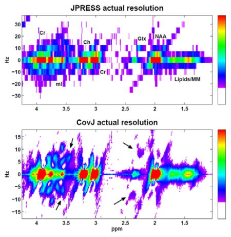
A maximum-echo sampled acquisition, as described above, was performed on 24 volunteers, and both JPRESS and CovJ data were obtained from this experimental data. Figure 5 shows localization of the medial, frontal gray region and also displays spectra from both JPRESS and CovJ techniques from a healthy, 63 year old volunteer. Contour plots of the two methods show qualitatively similar features, whereas improvement in spectral resolution is evident when comparing the true resolution spectra. For the CovJ spectra, off-diagonal peaks are displayed clearly for Glx and mI. In addition to the 2D spectral displays, 1D spectra can also be extracted from the CovJ data, as seen in Figure 6. These 1D spectra show unique lineshapes attributed to the diagonal and off-diagonal peaks for Glx as well as mI, and provide a more detailed display of these peak intensities.
Figure 5.

Localization is shown on the T1-weighted MRI in the axial (A), coronal (B), and sagittal (C) plane for a healthy, 63 year old volunteer. JPRESS and CovJ spectra extracted and processed from this location are displayed. Contour plots are shown on the left, whereas the actual resolution for the spectra can be seen on the right. On the CovJ spectrum, J-coupled signals appear as indicated with black arrows for Glx and mI.
Figure 6.

One dimensional spectra are extracted from the CovJ spectrum seen in the top left. Spectra were extracted from (black), the Glx peaks (red), and the mI peaks (purple).
JPRESS and CovJ spectra were also quantified using peak integration, yielding both metabolite concentrations and ratios with respect to Cr3.0 for the major metabolites of interest. Metabolite ratio means and CV % values are displayed in Table 1. For both methods, CV % was relatively similar and most metabolites had a CV % below 20%, with the exception of Lipids+MM. The mean values for both methods were nearly identical, however mI was significantly higher for the CovJ results (p<0.001). Upon inspection of mI in Figure 5, it is apparent that this elevation arises due to the off-diagonal peaks that form at for the CovJ spectra. This difference in mI/Cr3.0 does not necessarily imply that the CovJ method was ineffective at properly quantifying mI for each volunteer, however.
Table 1.
Ratios with respect to Cr3.0 are tabulated for 24 healthy volunteers (mean age = 64.7 years old) using both the JPRESS and CovJ methods. Data are displayed as mean values (CV% values) for all metabolites. mI/Cr3.0 was significantly higher using the CovJ method when compared to the JPRESS method (* = p<0.001), and this result is further explained in the text.
| Metabolite | JPRESS | CovJ |
|---|---|---|
| Lipids+MM | 1.23 (50%) | 1.31 (49%) |
| NAA | 1.21 (18%) | 1.20 (15%) |
| Glx | 1.62 (11%) | 1.63 (14%) |
| Ch | 0.32 (8.1%) | 0.33 (8.2%) |
| mI | 0.66 (8.9%) | 0.75 (11%)* |
Examining the concentration values for both methods provides insight into how well the CovJ method detects metabolites on a volunteer-by-volunteer basis relative to the JPRESS method. The correlation values (r2) between the CovJ and JPRESS peak integral concentrations were: 0.996 for Lipids + MM, 0.959 for NAA, 0.963 for Glx, 0.977 for Cr3.0, 0.979 for Ch, and 0.877 for mI. In addition, all correlation coefficients were found to be significant (p<0.001). These findings demonstrate that the CovJ method is essentially as effective as JPRESS in detecting changes in metabolic levels when peak integration is used for quantitation.
In addition to peak integration, prior-knowledge fitting was used to quantify Glu and GABA ratios with respect to Cr3.0 for both the JPRESS and CovJ methods. Figure 7 shows the 2.15–2.65ppm regions for the acquired CovJ spectrum, the fit of the CovJ spectrum, and the residual. Also, GABA and Glu ratios with respect to Cr3.0 are shown for all 24 healthy subjects using ProFit to quantify the JPRESS data and using Cov-SEHAR to quantify the CovJ data. The mean (CV %) values for GABA were 0.41 (50%) using ProFit and 0.14 (31%) using Cov-SEHAR. For Glu, the mean (CV %) values were 1.21 (18%) using ProFit and 1.27 (24%) using Cov-SEHAR. While no differences were seen between the two quantitation methods for quantifying Glu, a Student’s t-test demonstrated significant differences between the GABA results (p<0.001). (R2.1)
Figure 7.

The fit results using Cov-SEHAR are shown for a healthy control (age = 63 years old). The original acquired data, the fit, and the residual are shown on the top. Resulting GABA and Glu ratios with respect to Cr3.0 (wrt Cr3.0) are shown for all 24 healthy controls. ProFit results are displayed in red, whereas Cov-SEHAR results are displayed in black. The solid lines show the means of the data, and the dashed lines indicate the standard deviations of the data. While no statistical difference was found when comparing the Glu results, a Student’s t-test showed significant differences (p<0.001) between the ProFit and Cov-SEHAR results for GABA.
Discussion
The covariance J-resolved method, which implements the covariance transformation for processing JPRESS data, has been described and applied in vivo at 3T. The theoretical framework for this technique is similar to previously discussed covariance NMR theory [18, 19], and focuses on the relationship between FIDs across the indirect temporal direction, t1. Spectral points along F2 that are closely related will have similar phase modulations across the t1 FID depending on the experiment performed. Applying a covariance transformation to these points will therefore result in cross-peaks, or off-diagonal peaks, with higher amplitudes. This is in stark contrast to F2 points which are unrelated, as the covariance values of these t1 FIDs will usually be close to zero. Experiments such as TOCSY, which have high correlation values between F2 points, are ideal for utilizing the full potential of the covariance transformation.
Although, by employing a maximum-echo sampling scheme [16], it is also possible to use the covariance transformation on J-resolved spectra as demonstrated in this study. This sampling method not only improves overall sensitivity, but also induces a phase modulation along t1 that can be utilized to perform the covariance transformation effectively. This phase term is introduced due to the fact that chemical shift is not refocused when using maximum-echo sampling. Following the covariance transformation, it is possible to tilt the spectrum to the correct orientation by applying a phase modulation term, τ2, in the mixed (F2, ) dimension. This process does not result in any distortions to the lineshapes, however the spectral bandwidth is reduced by a factor of two. It is important to note that if the covariance transformation is applied after tilting the data by τ1, several false cross-peaks form due to the modified phase evolution along t1. Fortunately, the processing steps described in Figure 1 lead to an Scov matrix that is more representative of a JPRESS spectrum.
Simulations were used to show that the JPRESS and CovJ spectra have similarities, as well as differences originating from the unique processing steps of each method. The diagonal peaks ( ) are very similar when comparing the two methods, which is apparent in Figure 5. However, additional signal is added to the CovJ diagonal due to the fact that 𝒞ii points will have higher amplitudes than 𝒞ij points according to equation 1. For metabolites such as Lac, seen in Figure 2, the collapse of signal along the may be a potential disadvantage of the CovJ method. The mechanism behind cross-peak formation for the CovJ method, where the relationship between F2 points is spread into the dimension, has different effects depending on the strength of coupling. For strongly coupled spin systems [11], stronger cross-peaks are observed in Figure 2, whereas weakly coupled spin systems show suppressed cross-peak amplitudes. This is best demonstrated by mI (strong coupling) and Lac (weak coupling). Therefore, the CovJ method, in addition to improving spectral resolution, may also provide a unique contrast to the J-resolved spectrum based on coupling strength.
When comparing the cross-peaks from the two methods, it is important to note that the JPRESS indirect spectral dimension, F1, can be used to directly compute J-coupling between different resonances in high resolution NMR. Due to the mathematical nature of the covariance transformation, the physical value of J-coupling is lost in the dimension. Thus, the results suggest that the CovJ method is not appropriate for high resolution NMR, since the primary focus in this field is to actually quantify the J-coupling constants. For in vivo MRS, accurate J-coupling constants are not measurable unequivocally due to experimental complications, including line-broadening and low signal-to-noise ratios. Also, many metabolites of interest are strongly coupled spin systems, and therefore cross-peaks may reside very close to the diagonal peaks. For in vivo purposes, the spread of signal is more important than the physical J-coupling constant for the JPRESS method. Even though cross-peak structures are different between the JPRESS and CovJ techniques, CovJ still performs the primary responsibility of achieving spectral dispersion along the indirect dimension, as seen in Figure 5.
From a quantitative standpoint, it is apparent from the in vivo peak integration results that the two methods yield similar metabolic concentration and ratio values. Table 1 demonstrates that the ratios for most metabolites are nearly identical between the two methods, with the exception of mI. The increased mI ratio for CovJ is easily rationalized by observing that for in vivo spectra, seen in Figure 5, additional off-diagonal peaks are formed in the mI region at and . Since these peaks lie in the integration region for mI, the CovJ mI ratios are elevated when compared to the JPRESS mI ratios. In addition, the r2 correlation values associated with metabolite concentrations are very high, implying a strong linear relationship between the quantitative results of the two methods.
Since initial in vivo quantitative comparisons yield similar results, it is important to note that there are several potential advantages of the CovJ method that make it an attractive alternative, or addition, to the standard JPRESS method. Of course, the improved resolution along the indirect dimension is the main highlight of the CovJ technique. In order to have comparable resolution using JPRESS, the indirect dimensions would have to be zero-filled to t1 points = 1024. A direct comparison, seen in Figure 3, demonstrates that zero-filling to this resolution results in severe spectral ringing along the F1 domain; this is a well known drawback of the zero-filling method [17]. As mentioned above, CovJ off-diagonal peaks may change shape and location as a function of metabolite concentration, which is shown in figure 4. This is advantageous because the same peaks can now be modeled using additional parameters, such as distance between cross-peaks, which may further elucidate true metabolite concentrations. Therefore, it may be possible to further refine quantitation using these off-diagonal peak characteristics. (R2.2)
To investigate this potential advantage, the Cov-SEHAR prior-knowledge quantitation method was developed to quantify Glu and GABA from CovJ spectra and was compared to the standard ProFit algorithm, which fits JPRESS spectra [30]. ProFit utilizes both non-linear and linear fitting to model the 2D spectrum in order to provide accurate metabolite ratios with respect to Cr3.0. Since the addition of metabolites using CovJ is non-linear, Cov-SEHAR fits all parameters non-linearly, including concentration values. Furthermore, the spectral masking matrix (ℳ) aids in focusing the fit entirely on the cross-peaks of interest, which in this case were the cross-peaks that lie in between 2.15 and 2.65ppm. Figure 7 demonstrates that Glu results between the two quantitation methods are very similar. However, significant differences arise between the ProFit and Cov-SEHAR results for GABA. From these pilot findings, it appears that Cov-SEHAR results may be more stable when fitting data of varying spectral quality, demonstrated by lower CV % values. The Cov-SEHAR results are similar to previous reports regarding GABA in the human brain [30, 34, 35], whereas the ProFit results seem to be over-estimated. It is important to note that the original ProFit was used in this study, and a more detailed comparison study between ProFit 2.0 [31] and a refined Cov-SEHAR method is necessary before any definite conclusions can be drawn. (R2.1)
An important aspect of the CovJ method is that spectra are obtained using the same data necessary to produce JPRESS results: a(t2,t1). Therefore, no extra acquisition time and minimal additional processing steps are necessary to produce CovJ data. Thus, CovJ may be used as a subset of an existing JPRESS study, and can be used to validate findings from JPRESS quantitation without impacting the study protocol. In addition to J-resolved spectroscopy, the CovJ processing method can readily be applied to the constant-time PRESS (CT-PRESS) acquisition [15]. The only modification necessary for implementing this method is that S′ will be used as the final Scov matrix, since tilting is unnecessary for displaying the CT-PRESS spectra. Also, the CovJ method can be applied to multi-voxel J-resolved acquisitions, including experiments incorporating acceleration techniques [36, 37], on a voxel-by-voxel basis. Future studies will focus on utilizing the additional information provided in CovJ spectra to further enhance 2D JPRESS quantitation, and apply the CovJ method to multi-voxel J-resolved acquisitions.
Conclusion
A novel method for improving spectral resolution along the indirect dimension has been demonstrated for the single-voxel J-resolved spectroscopy experiment. Simulation and in vivo results have shown that while a number of qualitative differences exist between the two methods, including off-diagonal peak structure, the CovJ technique is still quantitatively similar to the JPRESS method when using peak integration. With the development of more advanced prior-knowledge fitting techniques, a combination of ProFit and Cov-SEHAR fitting may aid in the quantitation of metabolites in the future.
Acknowledgments
The authors would like to acknowledge the National Institute of Health R21 Grant (NS080648-02) and the University of California - Los Angeles Dissertation Year Fellowship Award (2016 – 2017).
List of Abbreviations
- 1D
One dimensional
- 2D
Two dimensional
- Asp
Aspartate
- Ch
Choline
- CovJ
Covariance J-resolved spectroscopy
- Cov-SEHAR
Covariance Spectral Evaluation of 1H Acquisitions using Representative prior-knowledge
- Cr3.0
Creatine 3.0
- Cr3.9
Creatine 3.9
- FT
Fourier transformation
- GABA
γ-aminobutyric acid
- Gln
Glutamine
- Glu
Glutamate
- Glx
Glutamate + Glutamine
- GSH
Glutathione
- JPRESS
J-resolved spectroscopy
- Lac
Lactate
- mI
myo-Inositol
- MM
Macromolecules
- MRS
Magnetic Resonance Spectroscopy
- NAA
N-acetyl aspartate
- NOESY
Nuclear Overhauser effect spectroscopy
- PRESS
Point-resolved spectroscopy
- SBW
Spectral bandwidth
- TOCSY
Total correlation spectroscopy
- VOI
Volume of Interest
References
- 1.Soares D, Law M. Magnetic resonance spectroscopy of the brain: review of metabolites and clinical applications. Clinical radiology. 2009;64:12–21. doi: 10.1016/j.crad.2008.07.002. [DOI] [PubMed] [Google Scholar]
- 2.Costello L, Franklin R, Narayan P. Citrate in the diagnosis of prostate cancer. The prostate. 1999;38:237. doi: 10.1002/(sici)1097-0045(19990215)38:3<237::aid-pros8>3.0.co;2-o. [DOI] [PMC free article] [PubMed] [Google Scholar]
- 3.Fischbach F, Bruhn H. Assessment of in vivo 1H magnetic resonance spectroscopy in the liver: a review. Liver International. 2008;28:297–307. doi: 10.1111/j.1478-3231.2007.01647.x. [DOI] [PubMed] [Google Scholar]
- 4.Boesch C, Slotboom J, Hoppeler H, Kreis R. In vivo determination of intra-myocellular lipids in human muscle by means of localized 1H-MR-spectroscopy. Magnetic Resonance in Medicine. 1997;37:484–493. doi: 10.1002/mrm.1910370403. [DOI] [PubMed] [Google Scholar]
- 5.Bolan PJ, Nelson MT, Yee D, Garwood M. Imaging in breast cancer: magnetic resonance spectroscopy. Breast Cancer Res. 2005;7:149–152. doi: 10.1186/bcr1202. [DOI] [PMC free article] [PubMed] [Google Scholar]
- 6.Bottomley PA. Spatial localization in NMR spectroscopy in vivo. Annals of the New York Academy of Sciences. 1987;508:333–348. doi: 10.1111/j.1749-6632.1987.tb32915.x. [DOI] [PubMed] [Google Scholar]
- 7.Ramadan S, Lin A, Stanwell P. Glutamate and glutamine: a review of in vivo MRS in the human brain. NMR in Biomedicine. 2013;26:1630–1646. doi: 10.1002/nbm.3045. [DOI] [PMC free article] [PubMed] [Google Scholar]
- 8.Provencher SW. Estimation of metabolite concentrations from localized in vivo proton NMR spectra. Magnetic Resonance in Medicine. 1993;30:672–679. doi: 10.1002/mrm.1910300604. [DOI] [PubMed] [Google Scholar]
- 9.Mescher M, Merkle H, Kirsch J, Garwood M, Gruetter R. Simultaneous in vivo spectral editing and water suppression. NMR in Biomedicine. 1998;11:266–272. doi: 10.1002/(sici)1099-1492(199810)11:6<266::aid-nbm530>3.0.co;2-j. [DOI] [PubMed] [Google Scholar]
- 10.Aue W, Bartholdi E, Ernst RR. Two-dimensional spectroscopy. Application to nuclear magnetic resonance. The Journal of Chemical Physics. 1976;64:2229–2246. [Google Scholar]
- 11.Ryner LN, Sorenson JA, Thomas MA. Localized 2D J-resolved 1 H MR spectroscopy: strong coupling effects in vitro and in vivo. Magnetic Resonance Imaging. 1995;13:853–869. doi: 10.1016/0730-725x(95)00031-b. [DOI] [PubMed] [Google Scholar]
- 12.Kreis R, Boesch C. Spatially Localized, One-and Two-Dimensional NMR Spectroscopy andin VivoApplication to Human Muscle. Journal of Magnetic Resonance, Series B. 1996;113:103–118. doi: 10.1006/jmrb.1996.0163. [DOI] [PubMed] [Google Scholar]
- 13.Thomas MA, Ryner LN, Mehta MP, Turski PA, Sorenson JA. Localized 2D J-resolved H MR spectroscopy of human brain tumors in vivo. Journal of Magnetic Resonance Imaging. 1996;6:453–459. doi: 10.1002/jmri.1880060307. [DOI] [PubMed] [Google Scholar]
- 14.Thomas MA, Yue K, Binesh N, Davanzo P, Kumar A, Siegel B, Frye M, Curran J, Lufkin R, Martin P, Guze B. Localized two-dimensional shift correlated MR spectroscopy of human brain. Magnetic Resonance in Medicine. 2001;46:58–67. doi: 10.1002/mrm.1160. [DOI] [PubMed] [Google Scholar]
- 15.Dreher W, Leibfritz D. Detection of homonuclear decoupled in vivo proton NMR spectra using constant time chemical shift encoding: CT-PRESS. Magnetic resonance imaging. 1999;17:141–150. doi: 10.1016/s0730-725x(98)00156-8. [DOI] [PubMed] [Google Scholar]
- 16.Schulte RF, Lange T, Beck J, Meier D, Boesiger P. Improved two-dimensional J-resolved spectroscopy. NMR in Biomedicine. 2006;19:264–270. doi: 10.1002/nbm.1027. [DOI] [PubMed] [Google Scholar]
- 17.Bartholdi E, Ernst R. Fourier spectroscopy and the causality principle. Journal of Magnetic Resonance (1969) 1973;11:9–19. [Google Scholar]
- 18.Brüschweiler R, Zhang F. Covariance nuclear magnetic resonance spectroscopy. The Journal of chemical physics. 2004;120:5253–5260. doi: 10.1063/1.1647054. [DOI] [PubMed] [Google Scholar]
- 19.Brüschweiler R. Theory of covariance nuclear magnetic resonance spectroscopy. The Journal of chemical physics. 2004;121:409–414. doi: 10.1063/1.1755652. [DOI] [PubMed] [Google Scholar]
- 20.Zhang F, Brüschweiler R. Indirect covariance NMR spectroscopy. Journal of the American Chemical Society. 2004;126:13180–13181. doi: 10.1021/ja047241h. [DOI] [PubMed] [Google Scholar]
- 21.Zhang F, Brüschweiler R. Spectral deconvolution of chemical mixtures by covariance NMR. Chem Phys Chem. 2004;5:794–796. doi: 10.1002/cphc.200301073. [DOI] [PubMed] [Google Scholar]
- 22.Trbovic N, Smirnov S, Zhang F, Brüschweiler R. Covariance NMR spectroscopy by singular value decomposition. Journal of Magnetic Resonance. 2004;171:277–283. doi: 10.1016/j.jmr.2004.08.007. [DOI] [PubMed] [Google Scholar]
- 23.Snyder DA, Zhang F, Brüschweiler R. Covariance NMR in higher dimensions: application to 4D NOESY spectroscopy of proteins. Journal of biomolecular NMR. 2007;39:165–175. doi: 10.1007/s10858-007-9187-1. [DOI] [PubMed] [Google Scholar]
- 24.Snyder DA, Xu Y, Yang D, Brüschweiler R. Resolution-enhanced 4D 15N/13C NOESY protein NMR spectroscopy by application of the covariance transform. Journal of the American Chemical Society. 2007;129:14126–14127. doi: 10.1021/ja075533n. [DOI] [PubMed] [Google Scholar]
- 25.Thomas MA, Iqbal Z, Sarma MK, Nagarajan R, Macey PM, Huda A. 2-D MR Spectroscopy Combined with 2-D/3-D Spatial Encoding. eMagRes. 2016;5:1039–1060. [Google Scholar]
- 26.Macura S, Brown LR. Improved sensitivity and resolution in two-dimensional homonuclear J-resolved NMR spectroscopy of macromolecules. Journal of Magnetic Resonance. 1983;53:529–535. [Google Scholar]
- 27.Smith S, Levante T, Meier BH, Ernst RR. Computer simulations in magnetic resonance. An object-oriented programming approach. Journal of Magnetic Resonance, Series A. 1994;106:75–105. [Google Scholar]
- 28.Govindaraju V, Young K, Maudsley AA. Proton NMR chemical shifts and coupling constants for brain metabolites. NMR in Biomedicine. 2000;13:129–153. doi: 10.1002/1099-1492(200005)13:3<129::aid-nbm619>3.0.co;2-v. [DOI] [PubMed] [Google Scholar]
- 29.Ogg RJ, Kingsley R, Taylor JS. WET, a T 1-and B 1-insensitive water-suppression method for in vivo localized 1 H NMR spectroscopy. Journal of Magnetic Resonance, Series B. 1994;104:1–10. doi: 10.1006/jmrb.1994.1048. [DOI] [PubMed] [Google Scholar]
- 30.Schulte RF, Boesiger P. ProFit: two-dimensional prior-knowledge fitting of J-resolved spectra. NMR in Biomedicine. 2006;19:255–263. doi: 10.1002/nbm.1026. [DOI] [PubMed] [Google Scholar]
- 31.Fuchs A, Boesiger P, Schulte RF, Henning A. ProFit revisited. Magnetic Resonance in Medicine. 2014;71:458–468. doi: 10.1002/mrm.24703. [DOI] [PubMed] [Google Scholar]
- 32.Iqbal Z, Wilson NE, Thomas MA. 3D spatially encoded and accelerated TE-averaged echo planar spectroscopic imaging in healthy human brain. NMR in Biomedicine. 2016;29:329–339. doi: 10.1002/nbm.3469. [DOI] [PubMed] [Google Scholar]
- 33.Van Belle G, Fisher LD, Heagerty PJ, Lumley T. Biostatistics: a methodology for the health sciences. John Wiley & Sons; 2004. [Google Scholar]
- 34.Prescot AP, Renshaw PF. Two-dimensional J-resolved proton MR spectroscopy and prior knowledge fitting (ProFit) in the frontal and parietal lobes of healthy volunteers: Assessment of metabolite discrimination and general reproducibility. Journal of Magnetic Resonance Imaging. 2013;37:642–651. doi: 10.1002/jmri.23848. [DOI] [PMC free article] [PubMed] [Google Scholar]
- 35.Ernst J, Böker H, Hättenschwiler J, Schüpbach D, Northoff G, Seifritz E, Grimm S. The association of interoceptive awareness and alexithymia with neurotransmitter concentrations in insula and anterior cingulate. Social cognitive and affective neuroscience. 2013;9:857–863. doi: 10.1093/scan/nst058. [DOI] [PMC free article] [PubMed] [Google Scholar]
- 36.Furuyama JK, Wilson NE, Burns BL, Nagarajan R, Margolis DJ, Thomas MA. Application of compressed sensing to multidimensional spectroscopic imaging in human prostate. Magnetic Resonance in Medicine. 2012;67:1499–1505. doi: 10.1002/mrm.24265. [DOI] [PubMed] [Google Scholar]
- 37.Wilson NE, Iqbal Z, Burns BL, Keller M, Thomas MA. Accelerated five-dimensional echo planar J-resolved spectroscopic imaging: Implementation and pilot validation in human brain. Magnetic Resonance in Medicine. 2016;75:42–51. doi: 10.1002/mrm.25605. [DOI] [PubMed] [Google Scholar]