Optimizing the performance of local canonical correlation analysis in fMRI using spatial constraints

Abstract

The benefits of locally adaptive statistical methods for fMRI research have been shown in recent years, as these methods are more proficient in detecting brain activations in a noisy environment. One such method is local canonical correlation analysis (CCA), which investigates a group of neighboring voxels instead of looking at the single voxel time course. The value of a suitable test statistic is used as a measure of activation. It is customary to assign the value to the center voxel for convenience. The method without constraints is prone to artifacts, especially in a region of localized strong activation. To compensate for these deficiencies, the impact of different spatial constraints in CCA on sensitivity and specificity are investigated. The ability of constrained CCA (cCCA) to detect activation patterns in an episodic memory task has been studied. This research shows how any arbitrary contrast of interest can be analyzed by cCCA and how accurate P‐values optimized for the contrast of interest can be computed using nonparametric methods. Results indicate an increase of up to 20% in detecting activation patterns for some of the advanced cCCA methods, as measured by ROC curves derived from simulated and real fMRI data. Hum Brain Mapp, 2012. © 2011 Wiley Periodicals, Inc.

INTRODUCTION

The benefits of locally adaptive statistical methods in fMRI have been shown only recently, as these methods more precisely detect brain activations in a noisy environment compared with mass‐univariate methods involving isotropic Gaussian smoothing [Borga and Rydell,2007; Friman et al.,2001; Harrison et al.,2007,2008; Harrison and Green,2010; Penny et al.,2005; Flandin and Penny, 2006; Rydell et al.,2008; Polzehl and Spokoiny,2001,2005; Ruttimann,1998; Sole et al.,2001; Tabelow et al.,2006; Walker et al.,2006; Weeda et al.,2009; Yue et al.,2010]. It has been suggested that conventional Gaussian smoothing in fMRI is intrinsically unsuitable as a technique to utilize the benefits of high resolution fMRI [Tabelow et al.,2009]. Locally adaptive statistical methods, however, take better advantage of high‐resolution data leading to enhanced signal detection capabilities without spatial blurring of edges of activation patterns because fine‐grained pattern information is not averaged over the local neighborhood defined by an isotropic smoothing kernel [Kriegeskorte and Bandettini,2007a,2007b]. With appropriate spatial filtering techniques, research studies can become more powerful and also render clinical applications more informative [Tabelow et al.,2009].

One such novel spatially adaptive method is local canonical correlation analysis (CCA), which investigates the joint time courses of a group of neighboring voxels instead of looking at the single voxel time course. CCA enables simultaneous adaptive spatial filtering and temporal modeling, and is thus a locally adaptive extension of the mass‐univariate general linear model (GLM). CCA and multivariate multiple regression are methodologically equivalent [Via et al.,2007]. In the past, different sets of spatial basis functions ranging from individual Dirac delta functions in a local neighborhood [Nandy and Cordes,2003a] to symmetric combinations of Dirac delta functions [Friman et al.,2001] were proposed using CCA. Other basis functions used were steerable spatial filter functions, which in analogy to the spherical harmonics form a complete angular set of functions and are thus able to adapt to an arbitrary direction in 2D or 3D coordinate space [Friman et al.,2003; Rydell et al.,2006].

Despite the increase of sensitivity using conventional CCA, the method is problematic to use in high‐resolution fMRI because of its low specificity (ability to classify nonactive voxels as not active) and increased susceptibility to artifacts [Nandy and Cordes,2004a]. In conventional CCA the value of a suitable test statistic is used as a measure of activation. It is customary to assign the value of the statistic to the center voxel of the local neighborhood. The method is prone to artifacts, especially in a region of localized strong activation. The reason for the increase in false activations is due to two different deficiencies of conventional CCA. The first deficiency is due to too much freedom of the spatial weights that allow for both positive and negative linear combinations of voxels. This freedom results in an improper spatial smoothing kernel combining low pass and high pass filter properties. The second deficiency is the so‐called bleeding artifact [Nandy and Cordes,2004a] which is a type of smoothing artifact. This artifact is expected to become stronger as the spatial constraint becomes less dominant for the center voxel. Simple approaches have been suggested previously to obtain a center voxel with sufficient dominant weight [Friman et al.,2001; Friman et al.,2003] to reduce the bleeding artifact but the specificity has never been systematically investigated. The bleeding artifact in connection with the shape of the filter kernel in CCA leads to a blocky appearance of activation patterns (block artifact). This artifact is most prominent for conventional CCA but can also arise when spatial constraints are used such that the weight of the center voxel is not enforced to be sufficiently dominant among all voxels in the neighborhood.

The potential benefit of using a spatial dominance constraint in CCA is that with a sufficiently large dominance condition of the center voxel the specificity can be increased and artifacts can be reduced or avoided. CCA with a spatial dominance constraint of the center voxel offers higher sensitivity and specificity than mass‐univariate methods with comparable Gaussian smoothing kernel.

In this research, we provide the mathematical framework to incorporate spatial dominance constraints in CCA to reduce artifacts and increase the specificity. We explicitly derive equations to solve the constrained CCA (cCCA) problem. For example, we investigate different constraints for the spatial weights on the ability to better detect activation patterns in the medial temporal lobes for an episodic memory task. Furthermore, we introduce a signed test statistic for cCCA that can handle any arbitrary linear contrast of interest. Using simulated and real data, we show the corresponding improvement of cCCA over conventional CCA and standard mass‐univariate approaches.

THEORY

CCA Formalism

Mathematically, CCA is a generalization of the GLM by allowing the incorporation of spatial basis functions according to

(1)

where the data are given by Y(ξ, t), ξ is the vector representing the spatial coordinates x, y, z, and t is time. The functions f _i(ξ), i = 1,…, p represent the spatial basis functions (local spatial filter kernels) modeling the spatial activation pattern in a neighborhood and the functions x _j(t), j = 1,…, r are the temporal basis functions modeling the hemodynamic response. The coefficients α_i and β_j are the spatial and temporal weights, respectively, that are being determined and optimized by the data for each individual neighborhood using an optimization routine. The symbol denotes spatial convolution and ε(t) is a Gaussian distributed random error term. If the number of spatial basis functions is reduced to a single function and this function is a simple Gaussian function with fixed width, i.e.,

we obtain the conventional GLM used in fMRI.

Local Neighborhood Approach

We are particularly interested in scenarios where the spatial basis functions are Dirac delta functions in a small local neighborhood such as a 3 × 3 pixel region [Nandy and Cordes,2003a]. With a small spatial filter kernel, cCCA has the potential to provide high specificity of the method and to avoid smoothing artifacts which are expected to increase with the size of the local neighborhood. Furthermore, using delta functions guarantees that edges of activation patterns are distinct and not blurred. In principle, the method easily can be extended to 3D by using a 3 × 3 × 3 voxel neighborhood, however, the computational effort is drastically increased, but today's GPU or other supercomputing resources can handle this complexity because each possible configuration can be processed independently of any other within the local neighborhood. Further justification of why a 2D 3 × 3 neighborhood is optimal is rooted in the 2D manifold structure of the gray matter sheet. The cortex always can be unfolded into a 2D sheet so that processing in the third dimension is not necessary.

Since Eq. (1) is linear we can use matrix notation. In the following we assume that the spatial basis functions are Dirac delta functions. Let Y be the matrix representing p voxel time courses with dimension t × p and X the conventional design matrix of size t × r for the r temporal regressors. Furthermore, let α and β be two unknown vectors of size p × 1 and r × 1, respectively. In conventional CCA, we look for the linear combinations of voxel time courses Yα and temporal regressors Xβ such that the correlation between both quantities is maximum. This leads to an eigenvalue problem with min(p, r) solutions from which the solution with the largest eigenvalue (i.e., maximum canonical correlation) is chosen.

cCCA and Dominance of the Center Voxel

Conventional CCA has a clear specificity problem [Nandy and Cordes,2004a], thus motivating the introduction of spatial constraints. However, with constraints, sensitivity will be decreased to some degree because specificity and sensitivity have opposite properties and cannot be maximized simultaneously. Furthermore, there exist an infinite number of possible spatial constraints and each constraint will have different sensitivity and specificity. We are particularly interested in linear and related constraints so that linear algebra can be used to find a solution of the cCCA problem. Besides obvious non‐negativity constraints of the spatial weights, of particular importance are spatial dominance constraints where the center voxel is guaranteed to be the largest among all other voxels in the local neighborhood. Spatial dominance, D, of all center voxels in the data can be defined by

where α${}_{\text{(}\mathit{\text{j}}\text{)}}^{\text{1}}$ is the weight of the j‐th center voxel, α${}_{\text{(}\mathit{\text{j}}\text{)}}^{\mathit{\text{i}}}$ is the weight of the i‐th voxel in the local neighborhood belonging to the j‐th center voxel, and the range of the min function contains all center voxels j in the dataset. If this dominance is infinite, we would have maximum specificity of the method and cCCA reduces to a mass‐univariate analysis. However, if the dominance is equal to one, we have weakest dominance which will provide maximum sensitivity but decreased specificity. In between these extremes, other important dominance constraints exist, and we will investigate one of them (the so‐called “strong dominance” or “sum” constraint) below and compare sensitivity and specificity to the weakest dominance constraint (the “maximum” constraint). We also consider the simple positivity constraint which is a nondominance constraint.

Constraints for cCCA

Let α be the vector of the spatial weights with components α_i and α₁ the weight of the center voxel of the local neighborhood. Then, we consider the following three constraints for cCCA:

Constraint #1 (simple constraint)

(2a)

Constraint #2 (sum constraint with strong dominance)

(2b)

Constraint #3 (maximum constraint with weakest dominance)

(2c)

If any of the α_i are zero, the corresponding voxel is excluded from the spatial configuration. Note, that Constraint #1 does not guarantee dominance of the center voxel. Constraint #2 (sum constraint) leads to a strong dominance of the center voxel whereas Constraint #3 (maximum constraint) leads to the smallest possible dominance of the center voxel.

All these constraints lead to a proper spatial smoothing (low pass filtering) because all components of α are larger than zero. A modification of Method #1 has been investigated in fMRI and found to be superior than unconstrained CCA [Friman et al.,2003; Ragnehed et al.,2009]. It can easily be shown [Das and Sen,1994] that Constraint #1 leads to the same algebraic equation as unconstrained CCA. Thus, the solutions of unconstrained CCA need only be searched over all possible voxel combinations satisfying Constraint #1 in each local neighborhood. Computationally, Method #1 is fairly easy to implement and with today's computing resources does not cause any problems in CPU time on a typical PC.

The disadvantage of Method #1 (and also of unconstrained CCA) is that the center voxel (to which the activation is assigned) is not guaranteed to have the maximum spatial weight, which could lead to potential artifacts. Method #2 has maximum specificity but may have less sensitivity compared to Method #3. Method #3 is quite different from the previous methods because the constraint is nonlinear and enforces least dominance of the center voxel leading to a high sensitivity but less specificity. Method #3 has the nice property that the coefficients are minimally restricted and at the same time satisfying the necessary positivity conditions with dominance of the center voxel D = 1.

We would like to point out that these constraints are not specific to the fMRI paradigms that we later investigate in this work. However, if largest specificity is of interest, a constraint with large dominance of the center voxel is expected to be more suitable. Similarly, for largest sensitivity, a constraint with the least dominance of the center voxel is expected to be best.

Solution of the cCCA Problem

To solve for linear constraints in α (Methods #2, #3), it is possible to linearly transform the α to a constraint equivalent to #1 by

(3)

such that satisfies a non‐negativity constraint

(4)

and M is an invertible transformation matrix. Observe, that now can also be zero which needs to be explicitly considered in the transformed space because voxel 1 (center voxel of neighborhood) can still satisfy the constraint in the original voxel space with a positive weight α₁ even when .

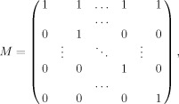
The transformation matrix M = (M _ij) for constraint #2, when Eq. (4) is satisfied, is given by

(5)

i. e. M _ij = 1 for i = j, M _1j = 1 for j ≥ 2, all other M _ij = 0.

The transform of α by M then leads to a transformation of the data Y to so that the spatial covariate becomes

where the transformed data are given by

and the maximum correlation between this covariate and Xβ needs to be found subject to the constraint on .

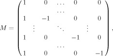
For Constraint #3, even though a nonlinear constraint, it is possible to find a transformation matrix. As shown in detail in Appendix A, the transformation matrix given by

(6)

will lead to a solution of cCCA for Constraint #3 when Eq. (4) is satisfied.

P‐Value Statistic

Each 3 × 3 neighborhood has 512 different configurations, of which 256 configurations have a center voxel. Once cCCA is performed for every 256 possible configurations in each 3 × 3 pixel neighborhood, we compute Wilk's Λ statistic by converting the cCCA problem into an equivalent multivariate multiple regression (MVMR) problem of the form

where Y are the data (size t × p), α is the optimum spatial weight vector (size p × 1), X is the design matrix (size t × r), B is the matrix of regression weights (size r × p), and E is a residual error matrix (size t × p). A likelihood ratio test for the null hypothesis

where C is a general contrast matrix of size w × r, leads to Wilk's Λ statistic given by

(7)

where the error matrix E_α and hypothesis matrix H_α are given by

respectively, and

is the least square solution [Rencher,1998]. Under normality assumptions and for any fixed α, Λ follows a Wilk's lambda distribution Λ(1, ν${}_{\text{H}{}_{\text{α}}}$, ν${}_{\text{E}{}_{\text{α}}}$), where ν${}_{\text{H}{}_{\text{α}}}$ = w are the degrees of freedom of the hypothesis matrix H_α and ν${}_{\text{E}{}_{\text{α}}}$ = t − r − p are the degrees of freedom of the error matrix E_α. If the contrast is a vector c, contrast reparameterization can be performed, and the first entry in c is a 1 and all other elements are 0 (see Appendix B). Wilk's Λ can be converted to a F statistic by [Rencher,1998]

(8)

and the negative logarithm of the significance (parametric P‐value) computed. Since our neighborhood around the center voxel is not uniform and can include from 1 to 9 voxels (due to the vanishing of spatial weights for the other voxels in the neighborhood depending on the particular constraint used), we compute the parametric P‐value according to Eq. (8) for all possible configurations in each 3 × 3 pixel neighborhood and find the particular configuration with lowest P‐value. This P‐value is then assigned to the center voxel. Please note that it is also possible to assign the value of the test statistic instead of the parametric P‐value of the test statistic to the center voxel. However, the test statistic is a biased measure because it does not include the size of the configuration. For example, a single voxel configuration with test statistic ω is far more significant than a multiple voxel configuration with the same value. Thus, a statistic based on the parametric P‐value adjusts automatically for the different sizes of voxel configurations and thus is a more unbiased measure of activation than the test statistic itself.

It is important to understand that this P‐value that is finally assigned to the center voxel should be treated as a statistic that quantifies the activation measure, rather than as a true P‐value, because assumptions of Gaussianity do not hold in general for fMRI data and, more critically, α is not a fixed vector in cCCA and the incorporation of constraints on the spatial weights α leads to a statistic that does not conform to any parametric distribution under the Null hypothesis. To compute the significance of the P‐value statistic, we use nonparametric methods involving resting‐state data. In a previous article we have introduced a novel nonparametric method that uses order statistics applied to resting‐state data to obtain the distribution of the maximum statistic [Nandy and Cordes,2007]. An implementation of this method provides accurate estimates of true P‐values adjusted for multiple comparisons. We briefly outline this method in Appendix C and point out some newly developed improvements that are not contained in the original article.

Signed Test Statistic For cCCA

We would like to point out that the statistic in Eqs. (7) and (8) can be easily converted to a signed univariate statistic (similar to the method proposed by Calhoun et al.,2004) if the contrast is a vector c. In this case we define Λ_± and F _± to be

(9a)

and

(9b)

respectively. With this definition, cCCA leads to a powerful analysis method providing signed test statistics which is not possible for multivariate test statistics such as the “searchlight” multivariate approach [Kriegeskorte et al.,2006]. The cost, however, is the necessity to use nonparametric significance testing because the parametric distribution is nontractable.

Optimum cCCA Solution Is a Function of the Contrast of Interest

The P‐value statistic introduced above will give the optimum solution of the cCCA problem as long as the contrast vector is reparameterized yielding only one transformed regressor. Reparameterization can be done as shown in Appendix B. Without reparameterization, it can be shown that only for unconstrained CCA the optimum α solution does not depend on the contrast matrix and the optimum α is equivalent to the α that gives the largest canonical correlation [Nandy et al.,2010]. For cCCA, such a relationship between the α that solves the cCCA problem and optimizes the MVMR problem for any contrast matrix of interest does not exist. Thus, to find the best solution, it is necessary to optimize the MVMR problem, and this solution will depend on the contrast matrix of interest. In the following we will derive the optimum solution: Consider a particular voxel configuration. Then the P‐value for this configuration will be optimal when Λ in Eq. (7) is minimized under the constraint of interest. This leads to the optimization function

(10)

where

and the function h(α₂, …, α_p) specifies the constraint of interest for α₁ such that α₁ ≥ h(α₂, …, α_p) according to Eqs. (2a, b, c). After linear transformation of α given by Eq. (3) using the transformation matrices of Eqs. (5), (6), Eq. (10) is of the same form as Eq. (A2) and leads immediately to the equivalent form, Eq. (A9), i.e.

where

Differentiation with respect to gives the conditions for the optimum solution of Eq. (10) yielding the generalized eigenvalue problem

where . Enforcing normalization using

provides

to be the solution of Eq. (10) in the transformed space and in the interior domain of . Inverse transform then leads to α^(s). Note that in order to be complete we also have to consider the α^(s) on the nontrivial α^(s) boundary as done before for constraint #3 [Eq. (A10)]. As an optimum solution of the cCCA problem we take the particular α that minimizes the parametric P‐value statistic of the contrast of interest. We would like to emphasize that the optimum spatial configuration is not just the largest canonical correlation between the spatial part and temporal regressors. It also depends on the contrast of interest and the size of the configuration. In fact, each different contrast produces a different optimal set of the weights α and β.

Significance and family‐wise error rate are computed nonparametrically, as outlined in Appendix C. Comparison to mass‐univariate analysis with Gaussian spatial smoothing is performed by using a FWHM = 2.24 pixels, as justified in Appendix D. To assess the performance of all analysis methods applied to real (nonsimulated) data, we use “modified ROC” techniques and reconstruct conventional ROC curves as outlined in Appendix E.

To illustrate the steps necessary to solve the cCCA problem and arrive at P‐values, we provide a comprehensive flowchart in Figure 1.

Figure 1.

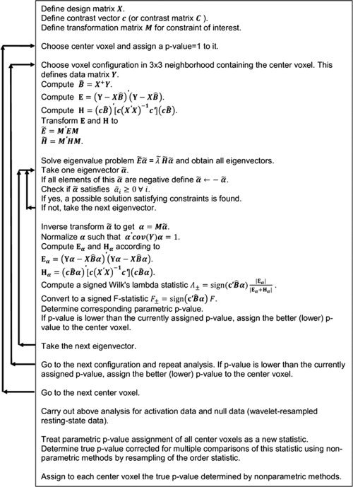
Flow chart to compute the p‐value for cCCA. This example fully describes the steps necessary to solve the cCCA problem with the sum (large dominance) constraint. Note that for each 3 × 3 neighborhood, there are 256 different spatial configurations possible that include the center voxel. Thus the loop over the configurations needs to be carried out 256 times for each center voxel. To solve the cCCA problem for the max (low dominance) constraint, an additional step (not shown in the flow chart) is necessary because solutions can also exist on the boundary of the α domain (see text).

MATERIALS AND METHODS

fMRI was performed for six normal subjects with IRB approval (according to institutional requirements) in a 3.0T GE HDx MRI scanner equipped with an 8‐channel head coil and parallel imaging acquisition using EPI with imaging parameters: ASSET = 2, ramp sampling, TR/TE = 2 s/30 ms, FA = 70°, FOV = 22 cm × 22 cm, thickness/gap = 4 mm/1 mm, 25 slices, resolution 96 × 96 reconstructed to 128 × 128 by zerofilling in k‐space. Three fMRI data sets were obtained for each subject (resting‐state, memory, motor) of which we only report the results of the first two in this article to avoid redundancy.

The first data set was collected during resting‐state where the subject tried to relax and refrain from executing any overt task with eyes closed. The light in the scanner room was shut off to avoid distracting the subject. Scan duration was 9 min 36 s and included 288 time frames.

The second data set was collected while the subject performed an episodic memory paradigm with oblique coronal slices collected perpendicular to the long axis of the hippocampus. Specifically, this paradigm consisted of memorizing novel faces paired with occupations. It contained six periods of encoding, distraction, and recognition tasks as well as short instructions. Words on the screen reminded subjects of the task ahead. Behavioral data were collected using a conventional 2‐button box with EPRIME (Psychology Software Tools, INC., Pittsburgh, PA). Specifically, the encoding task consisted of a series of novel stimuli (7 faces paired with occupations, displayed in sequential order for a duration of 3 s each, 21 s total duration) that the subject must memorize. After the encoding task a distraction task occurred for 11 seconds. The subject saw the letter “Y” or “N” in random order and random duration (0.5 to 2 s). The subject was instructed to focus on the “Y” and “N” and to press the right button whenever “Y” appeared and the left button whenever “N” appeared, as fast as possible. Reaction time and accuracy of the button presses were recorded. Because of its simplicity, this distraction condition functioned as an active control task and did not lead to any activation in regions associated with the memory circuit (hippocampal complex, posterior cingulate cortex, precuneus, fusiform gyrus). After the distraction task, the recognition task occurred consisting of 14 stimuli ‐ with half novel and half identical (in random order) to the stimuli seen in the previous encoding task (each stimulus was displayed for 3 s). The subject was instructed to press the right button if the stimulus was seen in the previous encoding task and press the left button if the stimulus was not seen (i.e., stimulus was identified as novel to the subject). Reaction time and accuracy of the button presses were recorded. In each of the six periods, different stimuli were used that the subject did not see before. Scan duration was 9 min and 36 s, and 288 time frames were collected. All face stimuli were taken from the color FERET database of photographs [Phillips et al.,2000].

The third data set was obtained by performing an event‐related motor task involving bilateral finger tapping while the subject was looking at a screen. The motor task lasted for 2 s and was alternated with a fixation period (serving as a control) of random duration lasting between 2 s and 10 s, uniformly distributed. Which task to perform was indicated on the display by the letter 1 for the motor task and 0 for the control task, programmed in EPRIME. Axial slices were collected with 150 time frames giving a scan duration of 5 min.

Data Analysis

All fMRI data were realigned in SPM5 (http://www.fil.ion.ucl.ac.uk/spm/), and maximum motion components were found to be less than 0.6 mm in all directions. In a preprocessing step, all voxel time series were high‐pass filtered by regression using a discrete cosine basis with cut‐off frequency 1/120 Hz [Frackowiak,2004]. No temporal low‐pass filtering was carried out. All voxels with intensity larger than 10% of the mean intensity were used in the analysis. This threshold effectively eliminated all nonbrain voxels leading to an average of about 4,500 voxels per slice.

Basis Functions for cCCA

All voxel time courses including the spatial basis functions and temporal regressors were mean subtracted (over time) and variance normalized. As local spatial basis functions in Eq. (1) we used Dirac delta functions in a 3 × 3 in‐slice neighborhood. This leads to 9 spatial filter kernels in Eq. (1) given by

such that i ^(k), j ^(k) = {1,1; 1,0; 1,−1; 0,1; 0,0; 0,−1; −1,1; −1,0; −1,1} [Nandy and Cordes,2003a]. For the temporal modeling, we specified design matrices as in SPM5 containing all conditions of the paradigms. In the memory paradigm we modeled instruction (I), encoding (E), recognition (R), and control (C) by temporal reference functions. In the motor paradigm, fixation (F) and motor task (M) were modeled according to the paradigm timings. All reference functions were convolved as usual with the standard SPM5 HRF two‐gamma function.

RESULTS AND DISCUSSION

Simulation

Spatial activation patterns (whose sizes range from 1 to 9 pixels) were generated on a 32 × 32 pixel grid (Fig. 2). Realistic pixel time series for the activation patterns were obtained from real motor activation data that were thresholded at P = 10⁻⁶ to obtain time series that are almost sure to be active with respect to the contrast “motor activation‐fixation”. To achieve a specific CNR, null data using wavelet resampled resting‐state data with intact correlation in time and space [see Bullmore et al.,2001; Breakspear et al.,2004] were added to all active and non‐active pixels of the simulated data in the 32 × 32 region. To compute the CNR we use the general definition

where λ_i and σ_i are the eigenvalues of the covariance matrix of the activation signal and noise, respectively [Cordes and Nandy,2007].

Figure 2.

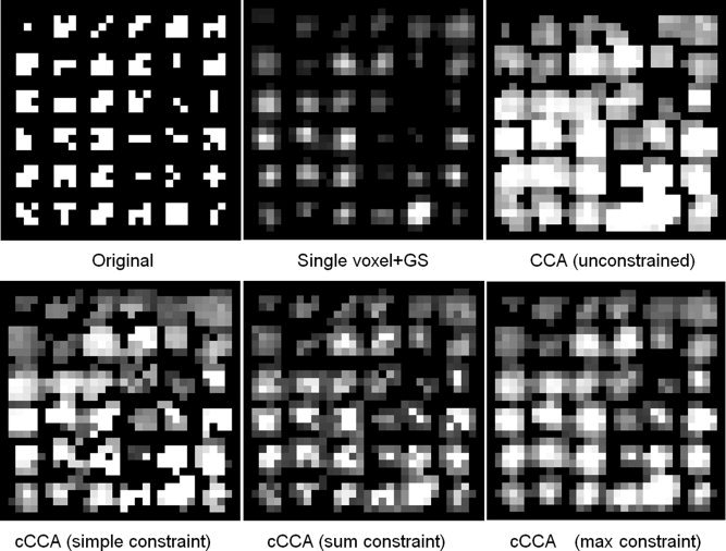
Spatial activation patterns (whose sizes range from 1 to 9 pixels) were generated in a 32 × 32 pixel region (top left). Realistic pixel time series for the activation patterns were obtained from motor activation data that were thresholded at P = 10^‐6 to obtain time series that are almost sure to be active with respect to the contrast “motor activation‐fixation”. To achieve a specific CNR, null data using wavelet resampled resting‐state data with intact correlation in time and space were added to all active and nonactive pixels of the simulated data in the 32 × 32 region. Spatial activation patterns are shown for CNR = 0.75 for different methods with P < 0.01 (uncorrected for multiple comparisons). Note the blurring of patterns for single voxel with Gaussian smoothing (FWHM = 2.24 pixels), strong bleeding and block artifacts for unconstrained CCA, block artifacts for cCCA with the simple constraint, but very small artifacts and accurate representation of most patterns by cCCA with the sum constraint, and good accuracy but some bleeding artifacts of cCCA with the maximum constraint.

To illustrate the performance of cCCA and appearance of different artifacts on a qualitative scale, we show in Figure 2 the spatial activation patterns for CNR = 0.75 for different methods with P < 0.01 (uncorrected for multiple comparisons). Note the blurring of patterns for single voxel with Gaussian smoothing (FWHM = 2.24 pixels), strong bleeding and block artifacts for unconstrained CCA, block artifacts for cCCA with the simple constraint, but very small artifacts and accurate representation of most patterns by cCCA with the sum constraint, and some bleeding artifacts of cCCA with the maximum constraint. Overall, cCCA with the sum constraint performs best followed by cCCA with the maximum constraint.

To quantify the performance of different methods, we show in Figure 3 conventional ROC techniques [i.e., fraction of true positives (FTP) vs. fraction of false positives (FFP)] for a high noise case (CNR = 0.25) (Fig. 3 left) and a low noise case (CNR = 0.5) (Fig. 3 right). Note that for the low CNR simulation the cCCA methods with the high and low dominance constraints are superior than the other methods, whereas for the high CNR simulation cCCA with the high dominance constraint is best. For both CNR scenarios conventional CCA performs poorly because of the strong bleeding artifact (see Fig. 2).

Figure 3.

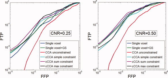
Conventional ROC techniques (fraction of true positives (FTP) vs. fraction of false positives (FFP)) are shown for the simulation of Figure 2. Specifically, a comparison was carried out for the high noise case (CNR = 0.25, left) and the low noise case (CNR = 0.5, right) using different analysis techniques. Note that for the low CNR case, the cCCA methods with the sum constraint and the max constraint are superior than the other methods whereas for the high CNR case, cCCA with the sum constraint is best. For both CNR scenarios conventional CCA (red) performs poorly. [Color figure can be viewed in the online issue, which is available at wileyonlinelibrary.com.]

Memory Activation in the Medial Temporal Lobes

Detection of memory activation in the medial temporal lobes, in particular in the hippocampus, is often complicated by the low CNR in the data. The primary source of difficulty is that hippocampal activations are weak and focal in nature, due to specialized task performance in hippocampal subregions (CA fields, dentate gyrus, subiculum) and nearby medial temporal lobe regions (entorhinal cortex, perirhinal cortex, parahippocampal gyrus, fusiform gyrus). Thus, it is problematic to see memory activations in the medial temporal lobes at stringent thresholds (for example P < 0.05 corrected for multiple comparisons) whether Gaussian spatial smoothing is performed or not using classical mass‐univariate methods, as they fail to harness systematic correlations in evoked responses within neighboring voxels. Locally adaptive methods based on cCCA can dramatically increase the sensitivity of detecting memory activations as shown in Figure 4A for the contrast “encoding‐control”. In this figure it is apparent that with single voxel analysis (without smoothing) no activation in the left hippocampus is visible. Furthermore, performing single voxel analysis with Gaussian smoothing eliminates almost all activations in bilateral hippocampal regions. Unconstrained CCA improves the detection of hippocampal activations but introduces severe artifacts as seen in the right parietal region. This artifact is less associated with the blocky appearance from the bleeding artifact but originates from the unconstrained signs of the spatial weights resulting in an enlarged subspace of voxel time series that correlate significantly with the memory regressors. This leads to a large fraction of false positives in null data and therefore gives a high threshold of the statistical map when a family‐wise error rate <0.05 is specified. The result is that hippocampal activations appear focal (a desirable feature) but are inherently unreliable because of the susceptibility of CCA to yield artifacts. The cCCA methods, however, do not have these weaknesses and show impressive detection of bilateral hippocampal activations with no apparent artifacts. If the threshold is lowered such that P < 0.001 uncorrected for multiple comparisons, detection of hippocampal activations is substantially increased by all methods (Fig. 4B). Unconstrained CCA now shows heavy artifacts in the right parietal cortex, and its activation patterns are not consistent with all other methods. Besides consistent hippocampal activations for all cCCA methods as well as univariate methods, cerebellar activations and bilateral activations in the fusiform gyrus are only clearly visible for the cCCA methods but not for mass‐univariate methods.

Figure 4.

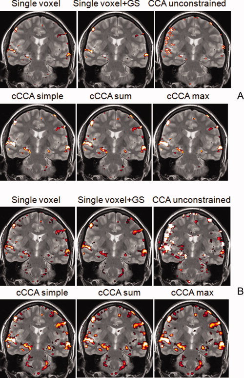
A: Activation maps with FWE < 0.05 for the memory paradigm using different analysis methods. The contrast is “encoding‐control”. B: Activation maps with P < 0.001 (uncorrected for multiple comparisons). [Color figure can be viewed in the online issue, which is available at wileyonlinelibrary.com.]

Reconstructed ROC Curves of Memory Activation

For data with low CNR, univariate analysis with or without Gaussian spatial smoothing performs poorly. This is reflected in a low sensitivity of mass‐univariate methods. Unconstrained CCA has larger sensitivity than single voxel analysis but very low specificity. Highest sensitivity is obtained by cCCA with the maximum constraint followed by cCCA with the sum constraint. It has been established that the modified ROC curves (see Appendix E) are always lower bounds of conventional ROC curves and that the ordinate of both ROC methods is linearly related for a given false positive fraction [Nandy and Cordes,2003b]. Thus, modified ROC curves provide an equivalent description to conventional ROC curves. Using the methods described in Appendix E [Eqs. (E1)–(E5)], we reconstructed conventional ROC curves for memory data (Fig. 5). Because of the linear relationship between both ROC techniques, the order of efficiency of different data analysis methods is the same but the magnitude of the efficiencies is increased by about 60% compared with modified ROC curves.

Figure 5.

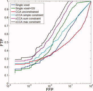
Reconstructed ROC curves using memory activation data for contrast “encoding‐control”. The x axis refers to a given fraction of false positives (FFP). The label FTP refers to the fraction of true positives. [Color figure can be viewed in the online issue, which is available at wileyonlinelibrary.com.]

Area Under the ROC Curves

Integrating the reconstructed ROC curves over FPF = [0,0.1], a range that is mostly important in neuroscience and radiology, provides a measure of overall performance of different data analysis methods. From Figure 6 we can conclude that cCCA with either the maximum constraint or the sum constraint have highest sensitivity. The degree of improvement compared to single voxel analysis with Gaussian spatial smoothing is about 20% for cCCA with the maximum constraint and 13% for cCCA with the sum constraint. This is true for both motor and memory fMRI data.

Figure 6.

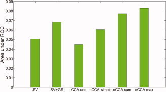
Area under the reconstructed ROC curve integrated from FFP = 0 to FFP = 0.1 for different data analysis methods. [Color figure can be viewed in the online issue, which is available at wileyonlinelibrary.com.]

Applicability of cCCA in fMRI

We predict that when analyzing data with small CNR (for example high‐resolution fMRI data), cCCA with the maximum constraint will maximize the method's sensitivity by ∼20% more than equivalent mass‐univariate approaches. The bleeding artifact will be less than with comparable mass‐univariate and Gaussian smoothing methods. If maximum specificity is desired (for example in neurosurgical mapping with fMRI), then cCCA with the sum constraint will yield optimum specificity (no significant bleeding artifact) with an increase in sensitivity of about 13%.

CONCLUSIONS

We summarize the ideas introduced in this study and results obtained

• 1We established the mathematical formalism of how constraints in cCCA can be handled by linear transformations and reduction of equations to the unconstrained CCA problem.
• 2We showed how to construct a signed statistic that accounts for any arbitrary contrast vector of interest and how to incorporate adjustments for different sizes of voxel configurations. Furthermore, we showed how to solve the cCCA problem by optimizing the weights α and β for a given contrast of interest.
• 3Constrained CCA methods lead to substantially increased detection of activation patterns for data with low CNR. In particular, for data with low CNR where the activation is thought to be localized to a small region such as episodic memory activation data, cCCA methods outperform conventional mass‐univariate analysis methods.
• 4If the constraint of cCCA does not guarantee dominance of the center voxel, block artifacts are observed (unconstrained CCA, cCCA with the simple constraint).
• 5Without constraint, CCA produces unreliable activation patterns because of the unrestricted sign of the spatial weights and very low specificity.
• 6Constrained CCA with the maximum constraint has the highest sensitivity but shows some bleeding artifacts in regions where the CNR is large. Compared to cCCA with the simple constraint and single voxel analysis with Gaussian smoothing, cCCA with the max constraint increases the statistical power by 20%.
• 7Constrained CCA with the sum constraint has no visible block artifacts nor bleeding artifacts. Compared to cCCA with the simple constraint and single voxel analysis with Gaussian smoothing, cCCA with the sum constraint increases the statistical power by 13%.

For these reasons we believe that advanced cCCA methods (using either the sum constraint for best specificity or the maximum constraint for best sensitivity) are superior to conventional CCA, cCCA with the simple positivity constraint, and mass‐univariate data analysis methods with or without Gaussian spatial smoothing in fMRI.

A. Solution of the Optimization Problem For the Maximum Constraint

The cCCA problem is equivalent to the regression problem

(A1)

such that

is the linear least squares (LS) solution (where X ⁺ is the pseudoinverse of X). Note that this β_LS is only up to a scale factor equivalent to the β in CCA because the β in CCA (β_CCA) satisfies the additional normalization condition [Rencher, 1998]

where the prime indicates “transpose”. Then, β_CCA is related to β_LS of the multivariate regression problem by

In the following we do not distinguish between these minor scaling differences of CCA and multivariate regression explicitly. Incorporating Constraint #3 using Lagrange optimization, leads to the following objective function to be minimized:

(A2)

where

(A3)

and λ, μ = (μ₁,…,μ_p), ν = (ν₁,…,ν_p) are Lagrange multipliers. The variables involving the components of ν are so‐called slack parameters and enforce that the spatial weights α₂,…,α_p are non‐negative and that α₁ ≥ max(α₂,…,α_p). The condition involving the variable λ

is an auxiliary normalization condition for vector α and is widely used in the classical theory of CCA [Rencher, 1998].

Differentiation of f(α,λ,μ,ν) with respect to ν and setting the result to zero yields

(A4)

Now, we need to consider the following two scenarios for α₁

(A5)

In the first case (i), ν₁,…,ν_p cannot be zero and it follows from Eq. (A4) that μ = 0. Then, Eq. (A2) reduces to the optimization condition for unconstrained CCA and can be easily solved. In the second case (ii), we obtain ν₁ = 0, and μ₂ = μ₃ = … = μ_p = 0 to be consistent with Eq. (A4). Thus, the objective function reduces to

Now, let

α_l = max (α₂,…,α_p) for some l ∈ {2,…,p}.

Then,

(A6)

needs to be minimized for all l ∈ {2,…,p} and the solution space searched for consistency with Eq. (A5). An elegant solution can be found by transforming Eq. (A6) to

(A7)

using Eq. (3) with

(A8)

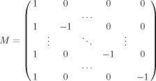
i.e., M _i1 = 1 for all i, M _ii = −1 for i > 1, and all other entries are zero. Note that M does not depend explicitly on the index l. The matrices and in Eq. (A7) are given by

where we have used the fact that M = M ⁻¹ for Eq. (A8). Then, needs to satisfy Eq. (4), and Eq. (A7) is equivalent to the unconstrained optimization problem because either or such that the derivative of f with respect to μ₁ yields the condition . In both cases the last term of Eq. (A7) vanishes, i.e. ,

yielding

(A9)

and Eq. (A9) is equivalent to unconstrained CCA. Thus, Constraint #3 leads to a single linear transformation, and the solution vector α obtained from needs to be checked if Constraint #3 is in addition satisfied. A search needs to be carried out over all possible voxel combinations in the local neighborhood due to the possibility that for any i ∈ {1,…,p}. The obtained solution space leads to a local minimum of function f in the interior region of the α domain. Thus, the solution space of α is given by Eq. (A10) such that all α and satisfy Eq. (A5) and Eq. (4).

In order for the solution space to be complete, we also have to consider that a possible minimum can occur at the (nontrivial) boundary of the α domain, which is given by

(A10)

Note, that the other constraints (#1, #2) do not have a non‐trivial boundary.

B. Contrast Reparameterization

For the memory paradigm, we present results for contrast E–C, whereas for the motor paradigm we are interested in the contrast M–F. These linear contrasts can be accommodated into the cCCA formalism by reparameterization of the design matrix X. For any linear contrast, the design matrix X can always be transformed to such that

(B1)

where X _eff is the first regressor of the new design matrix that is associated with a parameter estimate equivalent to the original contrast c ^′β. To compute X _eff we start with calculating the inverse of the design efficiency σ for an arbitrary contrast vector c:

(B2)

Then, the right hand side of Eq. (B2) can be written

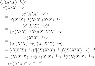Comparison with the left side of Eq. (B2) gives

For an alternative derivation see Smith et al. [2007]. The matrix X _⟂ in Eq. (B1) is perpendicular to X _eff and plays no role in the estimation of c ^′β.

C. Significance and Family‐Wise Error Rate

To determine the family‐wise error rate (FWE) nonparametrically for each subject we use resting‐state data as we previously proposed [Nandy and Cordes, 2007]. Resting‐state data are not null data but contain intrinsic structure (low frequency components) [Cordes et al., 2001]. Instead of correcting for the low frequency components using phase averaging [Nandy and Cordes, 2007] we use wavelet‐resampling in the temporal domain to obtain null data according to methods proposed by Bullmore et al. [2001] and Breakspear et al. [2004]. In the following section, we briefly summarize this method.

Let the test statistics at voxel ω be denoted by Y _ω. Then the family‐wise error rate is determined by the maximum statistic {max_ω Y _ω}, and for any threshold u, we can calculate the P‐value that automatically adjusts for multiple comparisons. To estimate the null distribution of {max_ω Y _ω}, we use the bootstrap method applied to the k largest order statistics {Y ⁽¹⁾,…,Y ^(k)} from wavelet resampled resting‐state data where we use the same (but random) permutation of wavelet coefficients in order to obtain resampled data where the spatial correlation of each resampled data set is exactly the same [Bullmore et al., 2001; Breakspear et al., 2004]. This method of wavelet resampling satisfies the criterion of exchangeability of fMRI time courses that are known to be spatially and temporally correlated. In the present context of cCCA, the relevant test statistic is given by Eq. ( 9a, b). We use standard nonparametric kernel‐density estimation techniques [Silverman, 1986] with a Gaussian kernel to obtain an estimate of the P‐value of this distribution. In order to make the statistic more uniform, we calculate the negative logarithm of the estimated P‐value, which we call Z. We then define

as normalized sample spacings for the k largest order statistics. If the observed samples at the voxels are exponential i.i.d., then so are the normalized sample spacings [Pyke, 1965]. This is true since the transformed test statistic is an exponential random variable by construction. The k largest order statistics can then be expressed as a linear function of the normalized sample spacings d _i and Z ^{(k + 1)} as follows:

Since d _i for i = {1,…,k} are i.i.d., we can use the bootstrap method to obtain resamples of normalized spacings d ${}_{\text{*}}^{\mathit{\text{i}}}$ for i = {1,…,k}. The latter can be used to generate resamples {Z ^*(1),…,Z ^*(k)} of the k largest order statistics from which the distribution of {max_ω Y _ω} can be obtained numerically. Since wavelet resampled resting‐state data can be considered to be null with respect to the temporal regressors used in this research, the obtained distribution approximates the null distribution of {max_ω Y _ω}. The chosen value for k was 100 for the bootstrap method and FWE was computed for P = 0.05.

D. Effective Filter Width

To compare results of cCCA with univariate methods involving Gaussian spatial smoothing, it is necessary to compute a comparable filter width (size of FWHM) of the Gaussian kernel from the size of the neighborhoods used in CCA. Since we are using all possible configurations in a 3 × 3 pixel area involving the center voxel and its 8 neighbors, the average configuration size is given by

A comparable Gaussian filter width is then specified by

We use this value for single voxel analysis with Gaussian spatial smoothing.

E. Receiver Operating Characteristics (ROC) Curves Using Real Data

The ROC method is a valuable tool for testing the efficiency of various data analysis methods and is usually used based on simulated data where the ground truth is known. This is acceptable for single‐voxel analysis because accurate modeling of spatial dependence of activation patterns between neighboring voxels is then not the most important aspect. However, for locally adaptive statistical methods the spatial structure of the data is most important and extremely difficult to model because the distribution of activated voxels is in general unknown, and simulated spatial patterns for more complicated tasks (such as episodic memory) are conceivably quite different from reality. We have shown in a previous article that the ROC method using simulated data can be modified and applied to real data [Nandy and Cordes, 2003b; Nandy and Cordes, 2004b] yielding so‐called “modified ROC curves”. In the following we briefly outline this method and point out two improvements. Instead of calculating the fraction of true‐positives (FTP) and fraction of false‐positives (FFP) based on ground‐truth data, we determine the fraction of active positives (FAP) (i.e. fraction of voxels detected to be active) using fMRI activation data and fraction of resting positives (FRP) using wavelet resampled resting‐state data, where, as before, we keep the spatial structure of the data by using the same (but random) permutation of the wavelet coefficients. From the quantities FAP and FRP, it is then possible to estimate FTP and FFP, as a function of the statistical threshold by

(E1)

where the letter P stands for probability, Y for an event indicating active detection, F for an event representing an inactive voxel. See Nandy and Cordes (2003b) for an explicit derivation of Eq. (E1). Thus, P(Y|T) is the probability of detecting a truly active voxel as active (FTP), P(T _A) is the fraction of truly active voxels, P(Y) is the fraction of voxels detected to be active (FAP), and P(Y|F) is the fraction of false positives (FFP). Since we only need to estimate fractions instead of the locations of active and nonactive voxels, it is not necessary to know the ground truth. The quantity FFP is readily estimated from the resampled resting‐state data because these data have null properties with respect to the paradigm. The quantity FAP is readily estimated from the activation data. Finally, an improved equation for P(T _A) can be derived based on P‐values [Nandy and Cordes, 2006]: Let N _A be the number of truly active voxels, k the number of voxels detected to be active and α the corresponding P‐value. Then N _A is bounded by

(E2)

yielding

(E3)

Thus,

(E4)

and the best estimate of P(T _A) is obtained by

(E5)

This result [Eq. (E5)] is more accurate than the approximation given in Nandy and Cordes [2003b]. For different analysis methods it is expected that the P(T _A) estimate is different because each method has different power. We use the average value of P(T _A) in order to be conservative.

With these estimations, modified ROC curves can be converted to conventional ROC curves. Finally, as a measure of performance we computed the area under the ROC curves (aROC), integrated over FFP∈[0,0.1], as a quantitative measure of activation in fMRI. We use as upper threshold FFP = 0.1 because in fMRI neuroscience we are more concerned in limiting the number of false positives than the number of false negatives. Furthermore, at FFP near 0.1 our experimental data show that the total error (false positives + false negatives) achieves a minimum. A similar approach in defining the thresholds for integration has been used by Skudlarski et al. [1999], Nandy and Cordes [2004b], and Ragnehead et al. [2009] before.

REFERENCES

- Borga M, Rydell J ( 2007): Signal and anatomical constraints in adaptive filtering of fMRI data In proceedings of IEEE International Symposium on Biomedical Imaging (ISBI'07), Arlington, Virginia, USA. [Google Scholar]
- Breakspear M, Brammer M, Bullmore E, Das P, Williams L ( 2004): Spatiotemporal wavelet re‐sampling for functional neuroimaging data. Hum Brain Mapp 23: 1–25. [DOI] [PMC free article] [PubMed] [Google Scholar]
- Bullmore E, Long C, Suckling J, Fadili J, Calvert G, Zelaya F, Carpenter T, Brammer M ( 2001): Colored noise and computational inference in neurophysiological (fMRI) time series analysis: Re‐sampling methods in time and wavelet domains. Hum Brain Mapp 12: 61–78. [DOI] [PMC free article] [PubMed] [Google Scholar]
- Calhoun VD, Stevens MC, Pearlson GD, Kiehl KA ( 2004): fMRI analysis with the general linear model: Removal of latency‐induced amplitude bias by incorporation of hemodynamic derivative terms. NeuroImage 22: 252–257. [DOI] [PubMed] [Google Scholar]
- Cordes D, Arfanakis K, Carew J, Haughton V ( 2001): Frequencies contributing to functional connectivity in the cerebral cortex in “Resting‐State” Data Am J Neuroradiol AJNR 22: 1326–1333. [PMC free article] [PubMed] [Google Scholar]
- Cordes D, Nandy R ( 2007): Independent component analysis in the presence of noise in fMRI. Magn Reson Imag 25: 1237–1248. [DOI] [PubMed] [Google Scholar]
- Das S, Sen P ( 1994): Restricted canonical correlations. Lin Algebra Appl 210: 29–47. [Google Scholar]
- Flandin G, Penny WD ( 2007): Bayesian fMRI data analysis with sparse spatial basis function priors. NeuroImage 34: 1108–1125. [DOI] [PubMed] [Google Scholar]
- Frackowiak RSJ ( 2004): Human Brain Function, 2nd ed. San Diego: Elsevier Science. [Google Scholar]
- Friman O, Cedefamn J, Lundburg P, Borga M, Knutsson H ( 2001): Detection of neural activity in functional MRI using canonical correlation analysis. Magn Reson Med 45: 323–330. [DOI] [PubMed] [Google Scholar]
- Friman O, Borga M, Lundberg P, Knutsson H ( 2003): Adaptive analysis of fMRI data. NeuroImage 19: 837–845. [DOI] [PubMed] [Google Scholar]
- Harrison LM, Penny W, Ashburner J, Trujillo‐Barreto N, Friston KJ ( 2007): Diffusion‐based spatial priors for imaging. NeuroImage 38: 677–695. [DOI] [PMC free article] [PubMed] [Google Scholar]
- Harrison LM, Penny W, Daunizeau J, Friston KJ ( 2008): Diffusion‐based spatial priors for functional magnetic resonance images. NeuroImage 41: 408–423. [DOI] [PMC free article] [PubMed] [Google Scholar]
- Harrison LM, Green GGR ( 2010): A Bayesian spatiotemporal model for very large data sets. Neuroimage 50: 1126–1141. [DOI] [PubMed] [Google Scholar]
- Kriegeskorte N, Goebel R, Bandettini P ( 2006): Information‐based functional brain mapping. Proc Natl Acad Sci USA 103: 3863–3868. [DOI] [PMC free article] [PubMed] [Google Scholar]
- Kriegeskorte N, Bandettini P ( 2007a): Analyzing for information, not activation, to exploit high‐resolution fMRI. NeuroImage 38: 649–662. [DOI] [PMC free article] [PubMed] [Google Scholar]
- Kriegeskorte N, Bandettini P ( 2007b): Combining the tools. Activation‐ and information‐based fMRI analysis. NeuroImage 38: 666–668. [DOI] [PubMed] [Google Scholar]
- Nandy R, Cordes D ( 2003a): A novel nonparametric approach to canonical correlation analysis with applications to low CNR functional MRI data. Magn Reson Med 49: 354–365. [DOI] [PubMed] [Google Scholar]
- Nandy R, Cordes D ( 2003b): Novel ROC‐type method for testing the efficiency of multivariate statistical methods in fMRI. Magn Reson Med 49: 1152–1162. [DOI] [PubMed] [Google Scholar]
- Nandy R, Cordes D ( 2004a): Improving the spatial specificity of CCA in fMRI. Magn Reson Med 52: 947–952. [DOI] [PubMed] [Google Scholar]
- Nandy R, Cordes D ( 2004b): New approaches to receiver operator characteristic methods in functional magnetic resonance imaging with real data using repeated trials. Magn Reson Med 52: 1424–1431. [DOI] [PubMed] [Google Scholar]
- Nandy R, Cordes D ( 2006): Nonparametric mixture modeling for mapping of brain activation using functional MRI data. Proceedings International Society of Magnetic Resonance in Medicine (ISMRM), Seattle, p. 2854. [Google Scholar]
- Nandy R, Cordes D ( 2007): A semi‐parametric approach to estimate the family‐wise error rate in fMRI using resting‐state data. NeuroImage 34: 1562–1576. [DOI] [PubMed] [Google Scholar]
- Nandy R, Jin M, Cordes D ( 2010): Extending the GLM for analyzing fMRI data to a constrained multivariate regression model. Human Brain Mapping conference, June 2010, Barcelona. [Google Scholar]
- Penny WD, Trujillo‐Barreto NJ, Friston KJ ( 2005): Bayesian fMRI time series analysis with spatial priors. NeuroImage 24: 350–362. [DOI] [PubMed] [Google Scholar]
- Phillips PJ, Moon H, Rizvi SA, Rauss PJ ( 2000): The FERET evaluation methodology for face recognition algorithms. IEEE Trans Pattern Anal Mach Intell 22: 1090–1104. [Google Scholar]
- Polzehl J, Spokoiny V ( 2001): Functional and dynamic magnetic resonance imaging using vector adaptive weights smoothing. J R Stat Soc Ser C 50: 485–501. [Google Scholar]
- Polzehl J, Spokoiny V ( 2005): Propagation‐separation approach for local likelihood estimation. Probab Theory Relat Fields 135: 335–362. [Google Scholar]
- Pyke R ( 1965): Spacings (with discussion). J Roy Statist Soc Ser B 27: 395–449. [Google Scholar]
- Ragnehed M, Engström M, Knutsson H, Söderfeldt B, Lundberg PJ ( 2009): Restricted canonical correlation analysis in functional MRI‐validation and a novel thresholding technique. Magn Reson Imaging 29: 146–154. [DOI] [PubMed] [Google Scholar]
- Rencher A ( 1998): Multivariate Statistical Inference and Applications. New York: Wiley. [Google Scholar]
- Ruttimann UE, Unser M, Rawlings RR, Rio D, Ramsey NF, Mattay VS, Hommer DW, Frank JA, Weinberger DR. 1998. Statistical Analysis of Functional MRI Data in the Wavelet Domain. IEEE Trans Med Imag 17: 142–154. [DOI] [PubMed] [Google Scholar]
- Rydell J, Knutsson H, Borga M ( 2006): On rotational invariance in adaptive spatial filtering of fMRI data. Neuroimage 30: 144–150. [DOI] [PubMed] [Google Scholar]
- Rydell J, Knutsson H, Borga M ( 2008): Bilateral filtering of fMRI Data. IEEE J Selected Topics Signal Process 2: 891, 896. [Google Scholar]
- Silvermann BW ( 1986): Density estimation for statistics and data analysis. New York: Chapman and Hall. [Google Scholar]
- Smith S, Jenkinson M, Beckmann C, Miller K, Woolrich M ( 2007): Meaningful design and contrast estimability in fMRI. Neuroimage 34: 127–136. [DOI] [PubMed] [Google Scholar]
- Sole A, Ngan SC, Sapiro G, Hu X, Lopez A ( 2001): Anisotropic 2‐D and 3‐D averaging of fMRI signals. IEEE Trans Med Imaging 20: 86–93. [DOI] [PubMed] [Google Scholar]
- Skudlarski P, Constable T, Gore J ( 1999): ROC analysis of statistical methods used in functional MRI: Individual subjects. NeuroImage 9: 311–329. [DOI] [PubMed] [Google Scholar]
- Tabelow K, Polzehl J, Voss HU, Spokoiny V ( 2006): Analyzing fMRI experiments with structural adaptive smoothing procedures. NeuroImage 33: 55–62. [DOI] [PubMed] [Google Scholar]
- Tabelow K, Piech V, Polzehl J, Voss H ( 2009): High‐resolution fMRI: Overcoming the signal‐to‐noise problem. J Neurosci Methods 178: 357–365. [DOI] [PubMed] [Google Scholar]
- Via J, Santamaria I, Perez J ( 2007): Deterministic CCA‐based algorithms for blind equalization of FIR‐MIMIO channels. IEEE Trans Signal Process 55: 3867–3878. [Google Scholar]
- Walker SA, Miller D, Tanabe J ( 2006): Bilateral spatial filtering: Refining methods for localizing brain activation in the presence of parenchymal abnormalities. Neuroimage 33: 564–569. [DOI] [PubMed] [Google Scholar]
- Weeda WD, Waldorp LJ, Christoffels I, Huizenga HM ( 2009): Activated region fitting: A robust high‐power method for fMRI analysis using parameterized regions of activation. Hum Brain Mapp 30: 2595–2605. [DOI] [PMC free article] [PubMed] [Google Scholar]
- Yue Y, Loh JM, Lindquist M ( 2010): Adaptive spatial smoothing of fMRI images. Stat Its Interface 3: 3–13. [Google Scholar]