

Abstract
latentnet is a package to fit and evaluate statistical latent position and cluster models for networks. Hoff, Raftery, and Handcock (2002) suggested an approach to modeling networks based on positing the existence of an latent space of characteristics of the actors. Relationships form as a function of distances between these characteristics as well as functions of observed dyadic level covariates. In latentnet social distances are represented in a Euclidean space. It also includes a variant of the extension of the latent position model to allow for clustering of the positions developed in Handcock, Raftery, and Tantrum (2007).
The package implements Bayesian inference for the models based on an Markov chain Monte Carlo algorithm. It can also compute maximum likelihood estimates for the latent position model and a two-stage maximum likelihood method for the latent position cluster model. For latent position cluster models, the package provides a Bayesian way of assessing how many groups there are, and thus whether or not there is any clustering (since if the preferred number of groups is 1, there is little evidence for clustering). It also estimates which cluster each actor belongs to. These estimates are probabilistic, and provide the probability of each actor belonging to each cluster. It computes four types of point estimates for the coefficients and positions: maximum likelihood estimate, posterior mean, posterior mode and the estimator which minimizes Kullback-Leibler divergence from the posterior. You can assess the goodness-of-fit of the model via posterior predictive checks. It has a function to simulate networks from a latent position or latent position cluster model.
Keywords: social network analysis, R, model based clustering, latent variable models
1. Introduction
Latent position models for social networks postulate an existence of an unobserved “social space” within which the probability of a tie between two actors is modeled as a function of some measure of distance between the latent space positions of these actors. Introduced by Hoff, Raftery, and Handcock (2002), these models were extended by Handcock, Raftery, and Tantrum (2007) to model grouping among actors as spherical Gaussian clusters in the latent space, and applied to non-binary data by Hoff (2005).
The R (R Development Core Team 2007) package latentnet implements the model described by Handcock et al. (2007), with slight modifications. The package implements Bayesian inference for the models based on an Markov chain Monte Carlo (MCMC) algorithm. It can also compute maximum likelihood estimates for the latent position model and a two-stage maximum likelihood method for the latent position cluster model.
As in Handcock et al. (2007), the package uses Minimum Kullback-Leibler (MKL) positions (Shortreed, Handcock, and Hoff 2006) for visualizing the posterior distribution of latent space positions and MKL label-switching algorithm (Stephens 2000) to deal with nonidentifiability of cluster assignments. It also adds support for nonbinary response variables, allowing them to be modeled as either binomial (with fixed, user-supplied number of trials) or Poisson.
This paper describes this package, and, as examples, fits two standard datasets. The first, Sampson’s “liking” network, among monks, is used an an example of a binary response. The second, the Highland Tribal alliances data, demonstrates nonbinary models. It is not the goal to describe all the functionality and options available, and more information about all of the commands and methods mentioned can be gotten through R’s help system.
The latentnet software itself is available from the Comprehensive R Archive Network (CRAN) at http://CRAN.R-project.org/package=latentnet and can be installed directly using, for example, install.packages(“latentnet”).
The latentnet package is part of the statnet suite of packages. The installer for the statnet suite installs all the required packages for you along with latentnet. It is easier for beginners or those interested in more general network models, visualization or simulation (including exponential family models).
1.1. Stochastic network models
We consider data on the relations between a set of n actors. The observations consist of a relational tie yi,j and covariates measured on each ordered pair of actors i, j = 1, …, n. In the most simple cases, yi,j is a dichotomous variable, indicating the presence or absence of some relation of interest, such as friendship, collaboration, transmission of information or disease, etc. Denote the n×n sociomatrix Y = [yi,j] and the dyadic covariates via the n × n × p array x = [xi,j,k]. In the case of a binary relationship we denote yi,j = 1 if there exists a relation from actor i to actor j, while yi,j = 0 will denote that no such directed relation exists. This can be thought of as a graph in which the nodes are actors and the edge set is {(i, j): yi,j = 1}.
The sociomatrix Y can be viewed as a random variable with a sample space of Y ⊆ {0, 1}n(n−1). We consider models for Pr(Y = y|x), the probability mass function of Y given the values of the covariates. Most papers in this special issues focus of statistical exponential family models (ERGM). In this paper we focus on a class of hierarchical models. The class of models assume that the conditional probability of a tie between two actors, given the covariates, depends only on the distance between them in an unobserved “social space.” The model also assumes that ties between actors occur independently, given their distance apart and the covariates.
1.2. Model specification
The model postulates that each actor has an unobserved position in a d-dimensional Euclidean latent social space. The most general form for the models fit by latentnet is
| (1) |
| (2) |
| (3) |
| (4) |
Intuitively, Z = {zi} are the positions in social space of the actors. Equation (1) states that the ties between individuals are independent, given the positions in social space of the two individuals. Here Zi ∈ ℝd is the d–dimensional location of the ith individual. Equation (2) states that the conditional probability depends on the covariates and latent positions only through their conditional mean given their distance apart and directed pair specific covariates. Equation (3) expresses this conditional mean in terms of a predictor function, ηi,j, and a known link function g. Equation (4) states that the predictor function is linear in the covariates and the distance apart. The package uses Euclidean distance, denoted by |Zi − Zj|, although other distances functions are possible.
Note that is slightly different from the specification of Handcock et al. (2007), in that latent space positions are not constrained and there is no multiplier for their distance. The specification in Handcock et al. (2007) is now implemented in latentnetHRT (see the section on “Package history” below).
The density-link combinations of (2)–(3) that are currently implemented are given in Table 1. For example, if the tie is dichotomous we can choose the Bernoulli family for the model. Then (2)–(3) specify a logistic regression model in which the probability of a tie depends on the Euclidean distance between Zi and Zj in social space:
where log odds(p) = log[p/(1−p)].
Table 1.
Response distribution families implemented in latentnet.
| Name | Family parameters | Density (Pr = f(y|μ)) | Link (η = g(μ)) | ||
|---|---|---|---|---|---|
| Bernoulli | (μ)y(1 − μ)1−y |
|
|||
| binomial | t = trials |
|
|
||
| Poisson |
|
log μ |
As in Handcock et al. (2007), when fitting in a Bayesian context, as an hierarchical model, prior distribution is imposed on the latent space positions and covariate coefficients, and hyperpriors on the latent space prior parameters:
Intuitively, the positions of the actors are drawn from a mixture of Gaussians. Each component of the mixture represents a difference group (i.e., class, category, type, etc) and the positions form a relative cluster of actors within the space. The model of Hoff et al. (2002) is essentially the case with G = 1.
Within this specification the user can specify d, G and the hyper parameters , ω2, . The prior density of the means is effected by ω2. The prior delineation of groups is controlled by and α. Larger values of the within-cluster variance ( ) lead to lower belief in cluster separation and a lower value of the within-cluster variance degrees of freedom (α) represents greater diversity in within-group variation.
The user can also specify the characteristics that influence the estimation algorithm. See Section 2.2 for details.
As part of the MCMC algorithm, an auxiliary variable K is introduced representing a hard clustering of latent space position within each iteration. This variable is useful computationally as the prior distribution can be reexpressed as:
1.3. Package history
The package latentnet was originally developed, by Mark S. Handcock, Peter Hoff, Susan Shortreed, and Jeremy Tantrum, to implement Handcock et al. (2007), but has been substantially rewritten by Pavel Krivitsky to enhance the capabilities and implement the new specification. The package latentnet implements the specification in this paper. To get the original specification in Handcock et al. (2007) use the package latentnetHRT. This corresponds to version 0.7 of the original latentnet.
2. Model specification and fitting
In this section, we describe how to fit latent position and latent cluster models for networks. This is done using the function ergmm.
The function ergmm constructs an internal representation of the model to be fitted, finds reasonable initial values for the MCMC algorithm, runs the MCMC sampler, and performs post-processing of the MCMC sample, returning an object of S3 class ergmm, described in Section 3.1.
The first, and the only mandatory, argument to ergmm is formula, to specify the network object to be used as the response variable in the model and the model to fit.
2.1. A simple motivating example
To get an idea of what the package can do we fit a standard data set in the social network literature. In 1968, Sampson collected data on 18 monks and their interpersonal relations (Sampson 1969). Each monk was asked about positive relations with the other monks and reciprocity was not required, thus the graph is directed. The data contain 56 directed ties between the 18 monks. There are no covariates in this data set, thus estimation is of a single covariate (the intercept) and the positions of the actors. The data is available in the package via the data function and a description can be found using the help function:
R> help(“sampson”)
R> help(“samplike”)
Let’s take a look at the names of the monks (followed by their order in the original):
R> data(“sampson”)
R> network.vertex.names(samplike)
[1]   “Romul_10”   “Bonaven_5”   “Ambrose_9”   “Berth_6”   “Peter_4”
[6]   “Louis_11”   “Victor_8”    “Winf_12”     “John_1”    “Greg_2”
[11]   “Hugh_14”    “Boni_15”     “Mark_7”      “Albert_16” “Amand_13”
[16]   “Basil_3”    “Elias_17”    “Simp_18”
and at the cohesive sub-groups designated by Sampson (1969).
R> samplike %v% “group”
[1]    “loyal”     “loyal”     “loyal”     “loyal”     “loyal”
[6]    “loyal”     “loyal”     “Turks”     “Turks”     “Turks”
[11]    “Turks”     “Turks”     “Turks”     “Turks”     “outcasts”
[16]    “outcasts”  “outcasts”  “outcasts”
We first fit a maximum likelihood estimator for a latent position model with two dimensions to the network samplike, using defaults for all other algorithmic inputs. The argument tofit is optional, telling ergmm that only the MLE is wanted, thus skipping the MCMC sampling run.
R> samplike.fit <- ergmm(samplike ~ latent(d = 2), tofit = c(“mle”))
Now list the maximum likelihood positions:
R> samplike.fit$mle$Z
           [,1]        [,2]
[1,] -2.7090545  3.28952923
[2,] -2.9528520 -0.07678311
[3,] -2.0116846  1.66519430
[4,] -5.8903989  1.13739904
[5,] -5.2390040  0.40541291
[6,] -3.7625123 -2.48585617
[7,] -1.6623223  1.73253755
[8,]  1.3414369 -2.12276851
[9,]  0.5937697 -0.67748534
[10,]  1.8756168 -1.41924228
[11,] -0.8315772 -3.13756229
[12,]  0.2393595 -4.10547804
[13,]  3.0012028 -1.71818716
[14,]  3.1875583 -3.67252510
[15,]  1.7019580  3.71005710
[16,]  4.1392687  2.23941286
[17,]  5.0562711  2.85642334
[18,]  3.9229640  2.37992166
Let’s plot them with the groups. First we create the plot symbols for the groups:
R> oneL <- samplike %v% “group”
R> oneL[oneL == “Turks”] <- “T”
R> oneL[oneL == “outcasts”] <- “O”
R> oneL[oneL == “loyal”] <- “L”
R> oneL[c(1, 7, 15)] <- “W”
R> oneL
[1]   “W”   “L”   “L”   “L”   “L”   “L”   “W”   “T”   “T”   “T”   “T”   “T”   “T”   “T”   “W”
[16]   “O”   “O”   “O”
Now create some colors:
R> oneLcolors <- c(“red”, “blue”, “black”, “green”) [match(oneL,
+     c(“T”, “O”, “L”, “W”))]
And finally plot the MLE positions and the groups:
R> plot(samplike.fit, label = oneL, vertex.col = oneLcolors,
+     what = “mle”, main = “MLE positions”, print.formula = FALSE,
+     labels = TRUE)
R> title(sub =
+     “Color represents the estimated groups, Labels the Sampson’s groups”)
The results are in Figure 1.
Figure 1.

MLE positions for a fit on Sampson’s Monks.
This quick fit and display creates as many questions as it answers. Did the algorithm converge? How well does the model fit? Are the MLE estimates good, or should alternatives be used? We will return to these later in the paper. But first let’s look at specifying more sophisticated models.
2.2. Model and prior distribution specification
Model formula
The first, and the only mandatory, argument to ergmm is formula, to specify the network object, defined in package network, to be used as the response variable in the model, and the covariates. This is done using the standard syntax for the statnet suite of packages: a two-sided R formula, with the response variable on the left-hand side and the covariates on the right-hand side, specified as function-like calls (Handcock, Hunter, Butts, Goodreau, and Morris 2003).
Terms that can be specified in the formula
Terms specific to latentnet are as follows:
Intercept By default, linear predictor ηi,j has at least an intercept term: x1,i,j ≡ 1. Adding a term “ -1” removes it. This is not recommended unless the other covariates are selected to make the intercept term redundant.
Latent space and clustering The term latent adds a Euclidean latent space distance term −|Zi − Zj | to the linear predictor of the probability of a tie between i and j, ηi,j, optionally modeling clustering of the latent space positions. The parameters to the term are as follows:
d (required) Dimensionality of the latent space d.
G (optional) Number of spherical Gaussian clusters into which the latent space positions are grouped G. The default is to fit a “plain” latent space model (G = 0).
var.mul, var (optional) Prior within-cluster variance .
var.df.mul, var.df (optional) Prior within-cluster variance degrees of freedom α.
mean.var.mul, mean.var (optional) Prior between-cluster variance ω2.
pK.mul, pK (optional) Prior Dirichlet parameter for cluster assignment probabilities, ν (same for all clusters).
For those parameters that have an argument ending in - .mul, the parameter can either be specified directly by passing the argument without the ending, or indirectly, by specifying the parameter with the ending, used as a scaling constant for picking a sensible prior. (This is the default.) See Section 2.4 for an explanation of how - .mul is used.
Other covariates An arbitrary dyadic covariate term can be added to the model by specifying xk,i,j directly with the term latentcov(x). The first argument, x, can either be a matrix of covariates for each dyad, or an edge attribute name of the response network. If an optional parameter attrname is specified, it is used as the user-visible name of the term. latentnet also implements all dyad-independent terms available in statnet. Note that the model does not admit terms which introduce conditional dyad-dependence.
In each term, it is possible to set prior mean (ξk) and variance ( ) using mean and var respectively. At this time, all covariate coefficients are modeled as a priori independent.
2.3. An example of a latent position fit with clustering
We next quickly fit a latent position model with two dimensions and three groups to the same network samplike, using defaults for all other algorithmic inputs. We first set the random number seed. This is not necessary but enables the results to be reproduced. The “seed” argument can be any integer, here 3141.
R> set.seed(3141)
The G parameter fits 3 groups. The optional argument verbose is used to make ergmm print out diagnostics of its progress:
R> samplike.fit <- ergmm(samplike ~ latent(d = 2, G = 3),
+     verbose = TRUE)
Generating initial values for MCMC:
Computing geodesic distances... Finished.
Computing MDS locations... Finished.
Computing other initial values... use of mclust requires a license agreement
see http://www.stat.washington.edu/mclust/license.txt
Finished.
Finding the conditional posterior mode... Finished.
Burning in... Finished.
Starting sampling run... Finished.
Post-processing the MCMC output:
Performing label-switching... Finished.
Fitting the MKL locations... Finished.
Fitting MBC conditional on MKL locations... Finished.
Performing Procrustes transformation... Finished.
R> summary(samplike.fit)
==========================
Summary of model fit
==========================
Formula:   samplike ~ latent(d = 2, G = 3)
Attribute: edges
Model:     Bernoulli
MCMC sample of size 4000, draws are 10 iterations apart, after
burnin of 10000 iterations.
Covariate coefficients posterior means:
       Estimate     2.5%    97.5% Quantile of 0
density 2.017285 1.330132 2.787141             0
Covariate coefficients MKL:
       Estimate
density 1.156569
2.4. Sensible prior for the hyper-parameters
The latent position model requires specifying a number of hyperpriors, and the model is sensitive to their choice. For example, too high a prior intra-cluster variance leads to clusters blurring together, while too low a prior intra-cluster variance creates a posterior mode in which all the clusters are concentrated at a point, causing the fit to “collapse”. For user convenience, latentnet implements a heuristic that produces adequate results on a variety of networks. The heuristic used is as follows:
In a typical network, ties even within a particular cluster form far from a complete graph, so the amount of space occupied by a cluster tends to increase with the number of nodes in the cluster, faster than a normal distribution with a fixed variance.
Intuitively, the node within each cluster needs a certain amount of space. The volume of a d-dimensional hypersphere is proportionate to its radius to the d’th power, so it makes sense to make the prior variance proportional to the d’th root of the cluster size.
For the dyadic covariate coefficients, the heuristic represents an a priori belief that coefficients of covariates with high magnitudes would, themselves, tend to have lower magnitudes to compensate. Thus, their respective prior variances are divided by the mean square of the covariate.
2.5. Controlling the fit and refining the computations
The control argument can be used to change the characteristics of the MCMC algorithm and how ergmm fits the given model. The control list is generated by the ergmm.control function (R has good reasons for this) in a similar fashion as glm.control (which can also be consulted for background).
All of these are passed as arguments to the ergmm.control function. For a simple list of these, type args(ergmm.control) in R, or for more information on each, type help(“ergmm.control”). Some of the more commonly used arguments include:
burnin The integer value assigned to this argument specifies how long the MCMC chain should proceed before beginning the sampling process. It also affects the length of the pilot runs for the adaptive sampling.
interval The integer value assigned to this argument specifies how long the MCMC chain should run between successive draws.
sample.size The integer value assigned to this argument specifies how many draws from the MCMC chain should be made.
2.6. Nonbinary edge weights
An ergmm call has two optional parameters, family and fam.par, to specify the model for the response variable; an optional argument response, giving either the name of the edge attribute to be used as a response or a sociomatrix, is also useful, since, at their core, the networks are binary. Currently implemented families are given in Table 1.
For example, consider the Highland Tribes dataset, available in the package netdata (Handcock et al. 2003) and sourced from UCINET (Borgatti, Everett, and Freeman 1999). These are 16 tribes in the Eastern Central Highlands of New Guinea, with each pair of tribes report to be in one of three states of relation: alliance, antagonism, or neutrality. While a multinomial model might be more appropriate, for the purposes of demonstration, we code alliance as 2, antagonism as 0, and neutrality as 1, and fit a binomial model with 2 trials. This dataset is included in latentnet, and this particular coding is contained in the network edge attribute sign.012. Thus, to fit this model, we use:
R> data(“tribes”)
R> tribes.fit <- ergmm(tribes ~ latent(d = 2, G = 3),
+     family = “binomial”, fam.par = list(trials = 2),
+     response = “sign.012”, verbose = 1)
3. Output format and visualization
In this section, we detail what the ergmm produces as output, how the summary function works, and how the plot function can be used to get sophisticated graphical representations of the model fit. Let’s start with the model output.
3.1. Class ergmm
Running ergmm produces an object of S3 class “ ergmm”, containing results of the run, diagnostic information, and some auxiliary data that can be used to reproduce it exactly. The entries returned depend on the relevant options passed to ergmm (i.e. the tofit argument):
sample is an object of class ergmm.par.list (detailed below), containing the parameter configurations drawn using the MCMC algorithm, as well as some diagnostic information such as acceptance rates of some of the Hastings proposals. It also has attributes Q, containing the posterior individual-node cluster assignment probabilities after label-switching, and breaks, containing information about which configurations came from which threads, in case of multi-threaded runs.
model is an object of class ergmm.model (see below), containing an internal representation of the model being fitted;
prior is an object of class ergmm.par, containing the information on the prior distribution used for the fit: its elements have names of the form var . par, where var is the variable whose prior distribution is being specified, and par is the name of the prior for this variable (the argument that would be passed to the term in the model formula). For example, Z.var gives the prior within-cluster variance for Z. This object can be passed as an argument to ergmm to produce a fit with an identical prior distribution. If used in this manner, it overrides any prior settings specified in the model formula.
control is a list of parameters that affect fitting but not the posterior distribution.
mcmc.mle and mcmc.pmode are objects of class ergmm.par, containing the highest-likelihood and highest-posterior-density MCMC sample encountered.
pmode is an object of of class ergmm.par, containing an approximate posterior mode (at this time, this posterior mode does not incorporate the prior cluster probability).
mle contains a maximum likelihood estimator.
mkl contains the configuration that minimizes Kullback-Leibler divergence between the predicted distribution and the posterior prediction.
burnin.start and main.start contain the configurations at which the burn-in and the sampling run, respectively, were started.
Storing parameter configurations: ergmm.par and ergmm.par.list
Each iteration of MCMC, as well as starting values, summary statistics, and hyperprior parameters are represented as instances of the ergmm.par S3 class, which extends the list class, primarily by disabling partial name matching. The correspondence between model parameters and elements of ergmm.par is given in Table 2.
Table 2.
Accessing parameter configurations in ergmm.par.
| Parameter | Name in ergmm.par | Packing |
|---|---|---|
| Z | Z | n × d matrix, with coordinates of individual node location in rows |
| β | beta | p-vector |
| μ | Z.mean | G × d matrix, with coordinates of individual cluster means in rows |
| σ | Z.var | G-vector |
| λ | Z.pK | G-vector |
| K | Z.K | n-vector |
A series of configurations, such as an MCMC sample, is stored in the ergmm.par.list class, which, in addition to providing access to the samples of individual variables using the $ operator, as with ergmm.par, also implements indexing using [[ ]] to extract individual configurations ( ergmm.par) and [ ] to extract subsets ( ergmm.par.list). This is analogous to indexing ordinary lists.
Class ergmm.model
A formula passed to ergmm is parsed into an internal representation of a network model, of class ergmm.model, containing the response network ( Yg), optional response attribute ( response), family and family parameters ( family and fam.par, respectively), the dimensionality of latent space ( d), number of clusters ( G), presence or absence of the intercept in the model ( intercept), and the number, names, and matrices of covariates ( p, coef.names, and x, respectively). This structure is returned as a part of an ergmm, and can be passed in place of a formulato rerun a particular model fit (though hyperpriors would need to be specified using the prior argument to ergmm).
A print method is available for ergmm.model, to pretty-print the information about an ergmm.model object.
3.2. Summarizing model fits
Although the results of latent position model fits are usually reported by plotting the latent space positions, latentnet does provide a convenient way to extract various summary statistics of the posterior. A summary method is implemented for ergmm objects, and returns an summary.ergmm object, which a print method available for it, or can be accessed as a list.
The method summary.ergmm takes the following arguments:
ergmm.fit (required) An object of class ergmm to summarize.
point.est (optional) Which point estimates to return; defaults to returning posterior mean ( “pmean”) and MKL ( “mkl”), but MLE ( “mle”) and posterior mode conditional on clustering ( “pmode”) are also available. quantiles (optional) For posterior mean, which quantiles to estimate. se (optional) Whether to compute standard errors for those point estimates for which they are available.
quantiles (optional) For posterior mean, which quantiles to estimate.
se (optional) Whether to compute standard errors for those point estimates for which they are available.
The resulting summary.ergmm object is a list containing the following elements:
ergmm is an object of class ergmm, containing the fit from which the summary was generated.
model is an object of class ergmm.model, containing the model that was fit.
pmean, mkl, mle, etc. are objects of class ergmm.par, containing the requested point estimates. Some of them also have an element Z.pZK, which contains the posterior probability each node being in each cluster; coef.table, which contains a data frame with the coefficients and, depending on the type of estimate, their standard errors or quantiles; and cor and cov, which contain the correlation and variance-covariance matrices of coefficient estimates, respectively.
For example, let’s take a look at the posterior probabilities of group membership for each monk.
R> attr(samplike.fit$sample, “Q”)
                       [,1]               [,2]                 [,3]
  [1,]  0.01928430  0.02366596  0.957049739
  [2,]  0.03843356  0.02808395  0.933482496
  [3,]  0.03402563  0.01792882  0.948045548
  [4,]  0.01124310  0.01698239  0.971774515
  [5,]  0.01082211  0.01401081  0.975167082
  [6,]  0.07754355  0.02568809  0.896768363
  [7,]  0.04183028  0.01961759  0.938552128
  [8,]  0.95588901  0.02259798  0.021513007
  [9,]  0.85877219  0.05536172  0.085866092
[10,]  0.94270104  0.03785835  0.019440603
[11,]  0.91075326  0.02499878  0.064247963
[12,]  0.95110659  0.02303133  0.025862077
[13,]  0.93486842  0.04493801  0.020193570
[14,]  0.92311048  0.02979315  0.047096364
[15,]  0.03827960  0.91644493  0.045275471
[16,]  0.03489295  0.95366667  0.011440381
[17,]  0.02770390  0.96321201  0.009084098
[18,]  0.03351011  0.95562972  0.010860164
One can see the polarization of probabilities, with most monks being assigned to a group with probabilities above 90%.
3.3. Plotting model fits
One of the most useful aspects of latent position models is that they provide a principled way to visualize the network of interest in 2 or 3 dimensions. The ergmm method plot does this, by feeding point estimates of latent space positions to network package’s plot.network function.
By default, a call to plot will plot the minimum Kullback-Leibler (MKL) estimates (see Shortreed et al. 2006, for the details) for:
R> plot(samplike.fit)
A convenient way to visualize clustering is by plotting each node as a small pie chart with the slices of the pie being the proportions of MCMC draws in which that node belonged to each cluster. This is done by passing pie=TRUE to the function. For better readability, we recommend using argument vertex.cex to increase the size of each plotting symbol, leading to the following code:
R> plot(samplike.fit, pie = TRUE, vertex.cex = 2.5)
The term vertex is used as a synonym for “node” here for consistency with the sna package. See Figure 2 for the resulting output.
Figure 2.

MKL positions for a fit on Sampson’s Monks. The pie charts on the right-hand plot show each vertex’s posterior probability of assignment to each cluster.
It is also possible to specify other point estimates using argument what. For example,
R> plot(samplike.fit, what = “pmean”)
and
R> plot(samplike.fit, what = “pmode”)
will plot the posterior means and the approximate posterior modes (if the latter were requested in the tofit argument to ergmm), respectively; while
R> plot(samplike.fit, what = 4)
will plot the positions from the 4’th MCMC draw. The latter is useful for diagnosing slow mixing, by placing it inside a loop with R function Sys.sleep:
R> for (i in 1:samplike.fit$control$sample.size) {
+       plot(samplike.fit, what = i)
+      Sys.sleep(0.1)
+  }
and thus producing an “animation” of the sampler’s evolution.
Plotting the Tribes fit is a little more complicated: to show whether an edge represents friendly a hostile relationship, the colors need to be specified manually. Here, edges representing alliances are green and enmities red:
R> plot(tribes.fit, edge.col = as.matrix(tribes, “gama”,
+        m = “a”) * 3 + as.matrix(tribes, “rova”, m = “a”) *
+        2, pie = TRUE)
4. Diagnostics and algorithm tuning
How well did the algorithm do in fitting the model? Is the MCMC algorithm “mixing”? Did it converge?
The quality and speed of the MCMC algorithm used to produce a Bayesian model fit depends on, among other things, the variances and the covariance structure of proposals. To help evaluate it, latentnet provides MCMC output diagnostics and uses adaptive sampling to tune the proposal parameters.
4.1. mcmc.diagnostics method for ergmm
A quick and easy way to view basic diagnostics for an ergmm fit is using mcmc.diagnostics method. This function uses the facilities of R package coda to compute Raftery-Lewis convergence diagnostics and plot autocorrelations, trace plots, and posterior density estimates for a subset of variables being simulated. Thus, to see if our fit to the binary monastery network mixed well, we can use
R> mcmc.diagnostics(samplike.fit)
which prints out the Raftery-Lewis diagnostic:
[[1]]
Quantile (q) = 0.025
Accuracy (r) = +/- 0.0125
Probability (s) = 0.95
             Burn-in     Total    Lower bound   Dependence
             (M)            (N)      (Nmin)             factor (I)
llk         30              7170    600                  12.0
beta.1    50             8670    600                  14.4
Z.1.1     100           20100  600                  33.5
Z.1.2     80             16060  600                  26.8
The plots produced by mcmc.diagnostics are in Figure 3. Similarly, with the Tribes,
Figure 3.

MCMC diagnostics for Sampson’s Monks fit.
R> mcmc.diagnostics(tribes.fit)
4.2. A simple proposal tuner
While it is usually easy to see if the sampler mixed well, finding those proposals that would produce good mixing is not trivial. Approaches based on the approximate posterior (such as Raftery and Lewis 1996) are not appropriate with the proposal types used, so a more empirical approach is used.
The burn-in is split into a series of pilot runs. A simple heuristic and user-supplied values are used to set the initial proposal parameters. After each pilot run, the acceptance rates are checked. If they fall below a very low threshold (or above a very high threshold), the pilot run is repeated with the proposal variances of the variables involved reduced (or increased) by a large factor. If they do not, the proposal standard deviations and coefficients are updated as follows:
For single-variable proposals, the proposal standard deviation is multiplied by the sample acceptance rate of the second half of the pilot run, and divided by the target acceptance rate.
For multivariate proposals, the empirical covariance in the second half of the pilot run of the variables involved is computed, its Cholesky decomposition is taken, and the resulting coefficients used to generate a multivariate normal proposal are multiplied by a scaling factor which is, again, multiplied by the sample acceptance rate and divided by the target acceptance rate.
These are then used by the next pilot run, or, if the burnin is over, in the sampling run. Following Neal and Roberts (2006), 0.234 is used as the default target acceptance rate.
5. Simulation of latent position and latent cluster networks
The package provides a way to simulate from an latent position model. This is straightforward, since at every level of the hierarchy, the model is dyad-independent. The model can be specified either by a formula or an ergmm object (typically a ergmm function model fit).
5.1. Simulation from the posterior of an ERGMM fit
The method simulate for ergmm fits simulates a network conditional on a random draw from the posterior. It is invoked simply by calling simulate with an ergmm object as its first argument. For example,
R> likemonks <- simulate(samplike.fit)
R> likemonks.par <- attr(likemonks, “ergmm.par”)
R> plot(likemonks, coord = likemonks.par$Z, edge.col = 8,
+       vertex.col = c(“red”, “green”, “blue”)[likemonks.par$Z.K])
with the output given in Figure 4.
Figure 4.
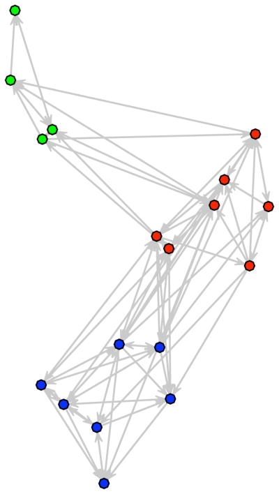
A random network generated from the posterior of the Sampson’s Monks fit.
Alternatively, it is possible to pass an ergmm.model object to simulate, along with the prior, specified as a list described in Section 3.1 , and a configuration of parameters, given as an ergmm.par object. The configuration of parameters does not need to have all the parameters specified: those missing will be generated from their prior distribution. For example,
R> likemonks1 <- with(samplike.fit, simulate(model,
+       par = sample[[1]], prior = prior))
R> plot(likemonks1)
will generate and plot a network from the first draw from the posterior.
Let’s now list the vector of posterior modal classes/clusters:
R> samplike.fit$mkl$Z.K
  [1] 3 3 3 3 3 3 3 1 1 1 1 1 1 1 2 2 2 2
and the positions
R> samplike.fit$mkl$Z
                        [,1]                [,2]
  [1,]  -0.34493014   -2.0132823
  [2,]  -0.45295050   -1.3742662
  [3,]   0.06573869   -1.8483487
  [4,]  -0.91224715   -2.4115134
  [5,]  -0.86635826   -2.0350114
  [6,]  -0.70346632   -1.1437845
  [7,]  -0.02661135   -1.5713670
  [8,]    1.26396550    0.7013976
  [9,]    0.73162392    0.4262798
[10,]    1.07428125    0.8078749
[11,]    1.15160197    0.3272236
[12,]    1.44923974    0.6933451
[13,]    1.19300715    0.9876187
[14,]    1.69374403    0.5699746
[15,]  -1.43794254    1.5082539
[16,]  -1.21039550    2.0844983
[17,]  -1.43313366    2.2544019
[18,]  -1.23516684    2.0367052
To assess uncertainty, we can plot some of the posterior distributions for the cluster mean positions:
R> plot(samplike.fit, what = “density”)
These appear in Figure 5.
Figure 5.
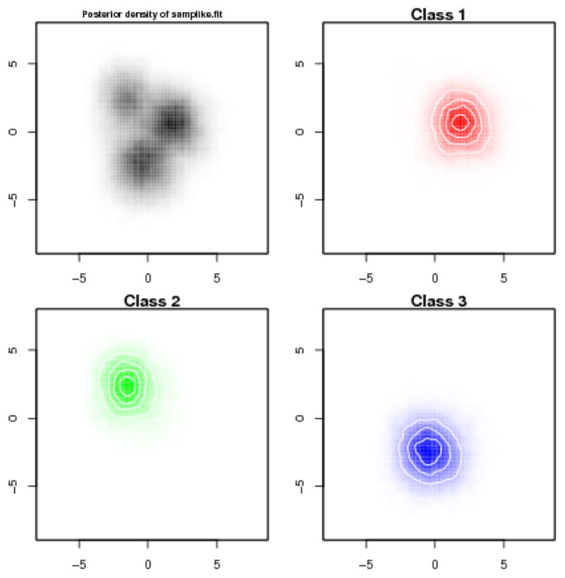
Two-dimensional posterior densities of cluster locations for Sampson’s Monks.
Finally, plot 24 versions of the positions in latent space to see how uncertain they are. This will not be plotted here as it takes many pages:
R> options(width = 65)
R> number.to.plot <- 24
R> interval.to.plot <- round(dim(samplike.fit$sample$Z)[1]/number.to.plot)
R> for (i in 1:number.to.plot) {
+       isamp <- 1 + (i - 1) * interval.to.plot
+       isamp.plot <- plot(samplike, label = ““, vertex.col =
+              samplike.fit$sample$Z.K[isamp,], arrowhead.cex = 0.3,
+              vertex.cex = 2, coord = samplike.fit$sample$Z[isamp, , ],
+              main = paste(“Draw number”, isamp))
+ }
6. Assessment of model fit via posterior predictive checks
As an assessment of the model fit we can consider posterior predictive checks. This is a goodness of fit method based on how similar the networks simulated from the posterior predictive distribution are to the original for some higher-order statistics of interest, such as the distribution of geodesic distances. To conduct such an analysis for the monk’s data we can use the gof function. The function specifies the higher-order statistics via a GOF formula. Any of those in the package ergm are available. The default statistics are idegree, odegree and geodesic distance.
R> samplike.fit.gof <- gof(samplike.fit)
To get a numerical summary:
R> summary(samplike.fit.gof)
Goodness-of-fit for in-degree
       obs min mean max MC p-value
0         0     0 0.08        1            1.00
1         0     0 0.34        2            1.00
2         3     0 1.10        4            0.18
3         5     0 2.76        7            0.28
4         1     0 3.51        8            0.26
5         3     0 3.63        8            0.94
6         2     0 3.33        8            0.64
7         1     0 1.76        7            1.00
8         1     0 0.96        3            1.00
9         0     0 0.43        4            1.00
10       1     0 0.06        1            0.12
11       1     0 0.03        1            0.06
12       0     0 0.01        1            1.00
Goodness-of-fit for out-degree
       obs min mean max MC p-value
0        0      0 0.04       1             1.00
1        0      0 0.43       2             1.00
2        0      0 1.46       4             0.42
3        1      0 2.56       6             0.52
4        5      0 3.15       7             0.34
5        7      0 3.81       7             0.10
6        5      0 2.88       7             0.30
7        0      0 2.03       6             0.28
8        0      0 1.23       5             0.58
9        0      0 0.25       3             1.00
10      0      0 0.12       2             1.00
11      0      0 0.03       1             1.00
12      0      0 0.01       1             1.00
Goodness-of-fit for minimum geodesic distance
        obs     min   mean max MC   p-value
1        88       60   87.91 105               0.94
2      136       98 137.65 170               0.88
3        77       31   62.75 103               0.28
4          5         0   11.76   42               0.74
5          0         0     2.13   21               1.00
6          0         0     0.40     9               1.00
7          0         0     0.08     3               1.00
Inf       0          0     3.32   56              1.00
To get a graphical summary we can use the plot function:
R> plot(samplike.fit.gof)
This produces three figures corresponding to in-degree distribution, out-degree distribution and geodesic distribution. Only the first figure, corresponding to the in-degree distribution is reproduced in the paper (Figure 6). We see that the model reproduces the observed statistics reasonable well except for the a tendency to somewhat under produce monks of degree 3 and over produce monks of degree 4. That is, there is a tendency for the actual monks to have degree 2 or 3 more often, and 4 less often than the model expects.
Figure 6.

A goodness-of-fit plot for Sampson’s Monks for the in-degree distribution of the monks. Note the envelopes and the disjunction between the proportions of monks with in-degree 3 and 4.
Acknowledgments
This research is supported by Grant DA012831 from NIDA and Grant HD041877 from NICHD.
Contributor Information
Pavel N. Krivitsky, University of Washington
Mark S. Handcock, University of Washington
References
- Borgatti SP, Everett MG, Freeman LC. UCINET 6.0 for Windows: Software for Social Network Analysis. Analytic Technologies; Natick: 1999. URL http://www.analytictech.com/ [Google Scholar]
- Handcock MS, Hunter DR, Butts CT, Goodreau SM, Morris M. statnet: Software Tools for the Statistical Modeling of Network Data. Statnet Project; Seattle, WA: 2003. http://statnetproject.org/ R package version 2.0, URL http://CRAN.R-project.org/package=statnet. [DOI] [PMC free article] [PubMed] [Google Scholar]
- Handcock MS, Raftery AE, Tantrum JM. Model-based Clustering for Social Networks. Journal of the Royal Statistical Society A. 2007;170(2):301–354. [Google Scholar]
- Hoff PD. Bilinear Mixed Effects Models for Dyadic Data. Journal of the American Statistical Association. 2005;100(469):286–295. [Google Scholar]
- Hoff PD, Raftery AE, Handcock MS. Latent Space Approaches to Social Network Analysis. Journal of the American Statistical Association. 2002;97(460):1090–1098. [Google Scholar]
- Neal P, Roberts G. Optimal Scaling for Partially Updating MCMC Algorithms. Annals of Applied Probability. 2006;16(2):475–515. [Google Scholar]
- Raftery AE, Lewis SM. Implementing MCMC. In: Gilks WR, Spiegelhalter DJ, Richardson S, editors. Markov Chain Monte Carlo in Practice. Chapman & Hall/CRC; London: 1996. pp. 115–130. [Google Scholar]
- R Development Core Team. R: A Language and Environment for Statistical Computing. R Foundation for Statistical Computing; Vienna, Austria: 2007. Version 2.6.1, URL http://www.R-project.org/ [Google Scholar]
- Sampson SF. PhD thesis. Cornell University; 1969. Crisis in a Cloister. [Google Scholar]
- Shortreed S, Handcock MS, Hoff P. Positional Estimation Within the Latent Space Model for Networks. Methodology. 2006;2(1):24–33. [Google Scholar]
- Stephens M. Dealing with Label Switching in Mixture Models. Journal of the Royal Statistical Society B. 2000;62(4):795–809. [Google Scholar]