Transmission characteristics of a two dimensional antiscatter grid prototype for CBCT

Abstract

Aim

High fraction of scattered radiation in cone‐beam CT (CBCT) imaging degrades CT number accuracy and visualization of low contrast objects. To suppress scatter in CBCT projections, we developed a focused, two‐dimensional antiscatter grid (2DASG) prototype. In this work, we report on the primary and scatter transmission characteristics of the 2DASG prototype aimed for linac mounted, offset detector geometry CBCT systems in radiation therapy, and compared its performance to a conventional one‐dimensional ASG (1DASG).

Methods

The 2DASG is an array of through‐holes separated by 0.1 mm septa that was fabricated from tungsten using additive manufacturing techniques. Through‐holes’ focusing geometry was designed for offset detector CBCT in Varian TrueBeam system. Two types of ASGs were evaluated: (a) a conventional 1DASG with a grid ratio of 10, (b) the 2DASG prototype with a grid ratio of 8.2. To assess the scatter suppression performance of both ASGs, Scatter‐to‐primary ratio (SPR) and scatter transmission fraction (Ts) were measured using the beam stop method. Scatter and primary intensities were modulated by varying the phantom thickness between 10 and 40 cm. Additionally, the effect of air gap and bow tie (BT) filter on SPR and Ts were evaluated. Average primary transmission fraction (T_P ) and pixel specific primary transmission were also measured for both ASGs. To assess the effect of transmission characteristics on projection image signal‐to‐noise ratio (SNR), SNR improvement factor was calculated. Improvement in contrast to noise ratio (CNR) was demonstrated using a low contrast object.

Results

In comparison to 1DASG, 2DASG reduced SPRs by a factor of 3 to 6 across the range of phantom setups investigated. Ts values for 1D and 2DASGs were in the range of 21 to 29%, and 5 to 14% respectively. 2DASG continued to provide lower SPR and Ts at increased air gap and with BT filter. Tp of 1D and 2DASGs were 70.6% and 84.7% respectively. Due to the septal shadow of the 2DASG, its pixel specific primary transmission values varied between 32.5% and 99.1%. With respect to 1DASG, 2DASG provided up to factor of 1.7 more improvement in SNR across the SPR range investigated. Moreover, 2DASG provided improved visualization of low contrast objects with respect to 1DASG and NOASG setups.

Conclusions

When compared to a conventional 1DASG, 2DASG prototype provided noticeably lower SPR and Ts values, indicating its superior scatter suppression performance. 2DASG also provided 19% higher average primary transmission that was attributed to the absence of interseptal spacers and optimized grid geometry. Our results indicate that the combined effect of lower scatter and higher primary transmission provided by 2DASG may potentially translate into more accurate CT numbers and improved contrast resolution in CBCT images.

1. Introduction

High scattered radiation intensity is one of the major causes of image quality degradation in flat‐panel detector (FPD) based cone‐beam CT (CBCT), which leads to loss of contrast resolution, reduced CT number accuracy, and scatter induced image artifacts.¹ Two major approaches, commonly known as scatter rejection and scatter correction methods, have been heavily investigated in the last decade to address this problem.^{2, 3, 4} For scatter rejection purposes, antiscatter grids (ASGs) developed for radiography and fluoroscopy have been employed in CBCT.^{5, 6, 7, 8, 9} These ASGs consists of a one‐dimensional array of radiopaque septa separated by aluminum or fiber spacers that support septa (such ASGs are referred as 1DASG in the rest of the text). 1DASGs typically provide a factor of 2 to 5 reduction in SPR values, and subsequently improve CT number accuracy and reduce image artifacts. Moreover, bow tie (BT) filters were also employed in CBCT, and they were shown to reduce scatter fraction in sections of the object close to the CBCT isocenter.^{5, 10, 11, 12, 13} While such scatter suppression devices help to reduce relative scatter intensity, residual scatter reaching the FPD is still high enough to deteriorate CBCT image quality. Scatter correction methods, which refers to correcting the effects of scatter after its detection by the image receptor, are often employed to correct the residual scatter.^{14, 15, 16, 17, 18, 19, 20, 21, 22, 23, 24} Generally, both of these approaches have been used together in CBCT systems for radiation therapy. However, the improvement in image quality is not at the desired level to achieve highly accurate CT numbers or improved visualization of low contrast objects.^{25, 26, 27, 28}

To improve scatter suppression in CBCT, 2DASGs may be a viable alternative to 1DASGs, since two‐dimensional septa can potentially provide better scatter rejection performance than one‐dimensional septa employed in 1DASGs. With recent advances in advanced manufacturing methods, 2DASGs were introduced for mammography,²⁹ breast tomosynthesis,³⁰ and multidetector CT (MDCT).^{31, 32} These 2DASGs were fabricated using lithographic techniques, and composed of copper (for mammography) or tungsten infused polymer (for tomosynthesis and MDCT) to achieve low septal thickness, high radio‐opacity, and geometric accuracy of the 2D grid. Moreover, due to the self‐supporting structure of a 2D grid, interseptal spacers were eliminated in 2DASGs, which may help to improve 2DASGs’ primary transmission properties.

To assess the feasibility of 2DASGs in the context of CBCT imaging, we designed and fabricated a 2DASG prototype to be employed in a linac mounted CBCT system. In contrast with 2DASGs cited above, our prototype was fabricated from pure tungsten using laser sintering based additive manufacturing methods. In this work, we evaluated its scatter and primary transmission characteristics under various imaging conditions, and compared it with a standard 1DASG employed in a clinical CBCT system. Additionally, we assessed the impact of transmission characteristics on the SNR improvement in projection images.

2. Materials and methods

2.A. 2DASG prototype

The 2DASG prototype was composed of a rectangular array of square, through‐holes, separated by tungsten septa (Fig. 1). To minimize the shadow of septa in projection images, through‐holes were aligned, or focused, in two dimensions toward the x‐ray source, and focusing geometry was matched to TrueBeam's “half‐fan” CBCT geometry (Varian Medical Systems, Palo Alto, CA, USA). It was composed of two, 2 cm wide by 20 cm long modules, and they were glued together to achieve 2 × 40 cm² coverage on the FPD plane. 2DASG has a grid pitch of 2.91 mm, grid height of 23 mm, and a septal thickness of 0.1 mm, resulting in a grid ratio of 8.2 (i.e., the ratio of grid height to through‐hole width). 2DASG was fabricated using the Powder Bed Laser Melting (PBLM) process, and it was manufactured by Smit Röntgen (Best, the Netherlands). PBLM process is similar to direct metal laser sintering,³³ where a computer guided laser beam driven by the CAD model of the ASG traces and melts the tungsten powder that is placed on a built platform. The grid structure is built on a layer‐by‐layer basis by lowering the platform, adding a new layer of tungsten powder, and repeating the laser melting process.

Figure 1.

Pictures of a 2 × 20 cm² 2DASG prototype, and the illustration of 2DASG. As better seen in the illustration, each grid hole has a unique slant, or angle, such that they are aligned toward the focal spot in half‐fan CBCT geometry. [Color figure can be viewed at wileyonlinelibrary.com]

2.B. Experimental setup and data acquisition

Experiments were performed using the CBCT system in a Varian TrueBeam STx linac. The CBCT system utilizes a PaxScan 4030CB FPD (Varian Medical Systems, Palo Alto, CA, USA) with an imaging area of 40 × 30 cm², and a GS‐1542 x‐ray tube (Varian Medical Systems, Palo Alto, CA, USA). In all experiments, half‐fan CBCT geometry (also known as offset detector geometry) was utilized (Fig. 2), where the center of FPD was shifted by 16 cm in the transverse direction with respect to imaging isocenter. Thus, the projected location of the beam's central axis (CAX) was 4 cm from the short edge of the FPD as indicated in Fig. 2. Projected location of CAX was simply referred as “CAX” in the rest of the text. In all experiments, central 2 × 40 cm² section of the FPD was exposed to x‐rays, and this section was referred as “measurement area” in the rest of text. The remainder of the FPD was covered with 3.2 mm thick lead sheet that blocked 99.7% of the primary beam. TrueBeam CBCT system comes with a focused, radiographic ASG (1DASG), that was composed of a 1D array of fiber interspaced lead septa. It has a grid ratio of 10, line rate of 60 l/cm, and septal thickness of 0.036 mm. In experiments with the 2DASG, 1DASG was removed, and the 2DASG was directly mounted on the protective cover of the FPD. Three different ASG configurations were evaluated: (a) Without ASG (NO ASG) (b) With 1DASG, (i.e., the standard ASG in TrueBeam CBCT) (c) With 2DASG.

Figure 2.

(Left) Side view of the experimental setup. Red circles correspond to measurement points, and they are located at CAX, 10 cm, and 20 cm off‐axis from CAX at detector plane. (Right) Beam eye view of the FPD. 2 × 40 cm² wide “measurement area” of the FPD is shown in gray. Rest of the FPD was covered with Pb sheet. [Color figure can be viewed at wileyonlinelibrary.com]

To modulate primary and scatter intensity, 30 × 30 cm² acrylic slab phantoms were employed (Table 1), and they placed on the carbon‐fiber treatment couch. The x‐ray source was positioned at “0” degree gantry angle, such that the central axis of the x‐ray beam was orthogonal to the couch surface. As described further in Section 2.D, scatter intensity was measured using lead beam stops, and they were placed between the phantom and the x‐ray tube. To better visualize the spatial variations in scatter intensity, beam stop measurements were performed at three different locations (at CAX, 10 and 20 cm lateral to CAX) as indicated by red circles in the detector plane.

Table 1.

Experiment setups used during primary and scatter transmission measurements

Setups	Phantom thickness (cm)	Air gap (cm)	BT filter
Setup 1	No object	N/A	No
Setup 2	0–40	20	No
Setup 3	20	20 and 35	No
Setup 4	20	20	Yes

All imaging experiments were performed at 125 kVp beam energy and with 0.9 mm thick built‐in titanium beam filter. The x‐ray tube was operated in pulsed mode, and tube current and pulse duration were adjusted to achieve sufficient signal intensity in images without saturating the FPD. As the measurement of scatter and primary signals assume linear and zero offset relationship between pixel values and absorbed energy, deviations from this assumption may bias scatter and primary signal measurements. In our preliminary investigations, we observed that pixel values could deviate from linearity more than 10%, when detector entrance exposure was below 0.01 mR/frame. To reduce the effect of nonlinear pixel response, detector entrance exposure was kept at a minimum of 0.1 mR/frame for 10–30 cm thick phantoms, where deviation of pixel values from linearity was 2%. With 40 cm thick phantom, detector entrance exposure was 0.05 mR/frame, where deviation from linearity was less than 5%.

The CBCT system comes with a built‐in monitor chamber placed on the x‐ray tube exit window; the output of the monitor chamber was used to normalize the image signal in projections due to changes in mAs settings and temporal variations in tube output. The FPD was operated at 2 × 2 pixel binning mode (i.e., pixel size: 0.388 mm). For each measurement, 50 frames were acquired, offset and flat field corrected, corrected for tube output variations, and averaged to reduce image noise. Corrected and averaged images were used in extraction of primary and scatter intensities as described in Sections 2.C and 2.D

2.C. Measurement of primary transmission

For primary transmission measurements, phantoms and the couch between the x‐ray source and FPD/ASG assembly were removed (Experiment setup 1 in Table 1), and two image sets were acquired: one with and one without an ASG. The ratio of images acquired with and without ASG yielded the primary transmission map. Average primary transmission fraction, (T_P), was obtained by averaging the values within a 1.6 × 1.6 cm² region of interest (ROI) in the primary transmission map,

$$T_P=\frac{I(withASG)}{I(withoutASG)}\times 100$$ (1)

where I is the average of pixel values within the predefined ROI. The center of the ROI was centered across the short edge (2 cm) of the measurement area, and shifted along the long edge (40 cm) to calculate T_P as a function of ROI location along the measurement area.

Since FPD pixels underneath the 2DASG's septa receive lower intensity of primary x‐rays, primary transmission varies spatially on a pixel‐by‐pixel basis, which was not reflected in T_P values. To evaluate this variation, primary transmission values extracted from the primary transmission map were presented in cumulative histograms, referred as primary transmission histograms (PTH).

2.D. Measurement of scatter transmission fraction and scatter‐to‐primary ratio (SPR)

For scatter intensity measurements, 3.2 mm thick, disc shaped Pb beam stops were mounted on a thin acrylic plate, between the phantom and the x‐ray focal spot (Fig. 3). Beam stops attenuated 99.7% of the primary beam, and the signal intensity in the beam stop shadow yielded the scatter intensity. In each beam stop shadow, a circular region of interest (ROI) was selected with a radius half of beam‐stop shadow's radius, and average scatter intensity, I_S, was calculated by averaging the pixel values within ROI. To keep the radii of beam stop shadows consistent across all scatter intensity measurements, the beam stop tray was placed at 85 cm from the x‐ray focal spot. This way, magnification of beam stop shadows were kept constant at the detector plane.

Figure 3.

SPR (a) and T_S (b) values for 20 and 40 cm thick phantoms were plotted as a function of beam stop diameter. Linear fits were used to extrapolate SPR and T_S values to “0” beam stop diameter. Measurement were performed at 10 cm from CAX, and using Experiment Setup 2 in Table 1. [Color figure can be viewed at wileyonlinelibrary.com]

For Scatter‐to‐Primary ratio (SPR) measurements, two sets of images were acquired at each experiment setup (Setups 2–4 in Table 1), one with and one without beam stops. SPR was calculated using following,

$$SPR=\frac{I_S}{I_{P+S}-I_S}$$ (2)

I_S was obtained from images with beam stops as described above, whereas scatter plus primary intensity, I_P+S, was obtained by averaging the image signal at the same ROI location in images acquired without beam stops. To quantify the scatter suppression difference between the 1D and 2DASGs, SPR reduction factor was calculated, which was the ratio of SPRs measured with 1D and 2DASGs.

Scatter Transmission fraction, Ts, is the fraction of scatter intensity transmitted through an ASG, and it is a key metric in quantifying the scatter suppression performance of ASGs. Ts was calculated using the following,

$$T_S=\frac{I_S(withASG)}{I_S(withoutASG)}\times 100$$ (3)

where I_S was obtained from images acquired with and without ASG in place.

As the beam stop size affects scatter intensity, SPR and T_S measurements were performed using four different diameter beam stops (their diameters were 3.5, 7.2, 10.5, and 13.6 mm at the detector plane), and they were linearly extrapolated to “0” beam stop diameter by using least squares polynomial fitting.^{34, 35, 36} In the Results section, SPR and T_S values at “0” beam stop diameter, and their standard errors were presented. An example of measured SPR and Ts values versus beam stop diameter was shown in Fig. 3. The data were measured using 20 and 40 cm thick phantoms. Y‐axis intercepts of linear fits yielded “0” beam stop diameter SPR and Ts values.

The effect of air gap on SPR and Ts was evaluated using 20 and 35 cm air gaps, and 20 cm thick phantom (Experiment setup 3 in Table 1). Air gap was the distance between the bottom surface of the treatment couch and the FPD plane. The effect of half‐fan BT filter was evaluated using 20 cm thick phantom and 20 cm air gap (Experiment setup 4 in Table 1).

2.E. Improvement in signal to noise ratio

Improvement of low contrast object visualization in CBCT images is important as high scatter fraction degrades signal to noise ratio (SNR) in CBCT projections, and subsequently affects low contrast visualization in CBCT images.¹ The methodology to evaluate the effect of ASGs on SNR has been developed by several authors in the past,^{35, 37, 38, 39} and it has been utilized in the context of CBCT.^{7, 8, 10} SNR for a contrast object is defined as

$$SNR=\frac{cP}{{(P+S)}^{0.5}}$$ (4)

where P is primary intensity, S is scatter intensity, and c is a multiplicative factor that defines the primary intensity difference, cP, between the contrast object and the uniform background.³⁵ In evaluation of ASG's impact on SNR, SNR improvement rather than the SNR value by itself, has been assessed.^{10, 39} Thus, SNR improvement factor, K_SNR, was employed in our study, which is the ratio of SNR with ASG to SNR without ASG. K_SNR was calculated as,³⁵

$$K_{SNR}=\frac{T_P{(1+SPR)}^{0.5}}{{(T_P+T_{S}SPR)}^{0.5}}$$ (5)

where SPR was measured without ASG. K_SNR more than 1 indicates that the use of ASG increases SNR with respect to SNR without an ASG at a given SPR value, whereas K_SNR less than 1 indicates that the ASG reduces the SNR. K_SNR for both ASGs were calculated from measured SPR, T_S, and T_P values described in Sections 2.C and 2.D.

2.F. Demonstration of low contrast object visualization

To demonstrate the improvement in CNR in projection images, a low contrast phantom was fabricated by drilling an array of five holes in 2.5 cm thick acrylic phantom. Holes were 0.6 cm in diameter and their depth varied from 2.5 to 0.5 cm in 0.5 cm increments. Contrast phantom was placed directly on the treatment couch, and phantom thickness was increased to 20 and 40 cm by adding acrylic slabs. This way, the contrast object magnification was kept constant at different phantom thicknesses. With each grid configuration, two image sequences were acquired, one with and one without the contrast phantom. The sequence without the contrast phantom was used for flat field correction of the contrast phantom images. CNR for the highest contrast object was calculated using the following,

$$CNR=\frac{|C-B|}{\frac{1}{2}({\mathit{\sigma }}_C+{\mathit{\sigma }}_B)}$$ (6)

where C and B are the mean pixel values in ROIs located in the contrast object and background, respectively, σ _C and σ _B are their corresponding standard deviations. For each experiment setup, mean and standard deviation of CNR was calculated over 50 image frames. To demonstrate the effect of exposure on CNR, phantom images were acquired at two different exposure levels. Detector entrance exposure was measured using a RaySafe Solo exposure meter (Unfors RaySafe, Cleveland, OH, USA), placed above the ASG/FPD assembly.

3. Results

3.A. Primary transmission

Figure 4(a) shows a section of the primary transmission map of the 2DASG, where brighter and darker regions correspond to through‐holes and septa of the 2DASG, indicating higher and lower primary transmission values, respectively. The orange square shows an ROI that was used for calculation of Tp. Tp as a function of ROI location along the measurement area is shown in Fig. 4(b). The mean (and standard deviation) of Tp across all ROI locations were 70.6 ± 0.2% and 84.7 ± 0.4% for 1D and 2DASG respectively. A slight reduction in 2DASG's Tp is visible at 20 cm. This location corresponds to the abutment surface of the two 2DASG modules, where the septal thickness was doubled (i.e., 0.2 mm). Thus, ROIs that included the location of the abutment surface had relatively lower T_P values.

Figure 4.

(a) A section of the primary transmission map of 2DASG is shown, where bright and dark regions indicate higher and lower primary transmission values respectively. The orange colored square indicates a 1.6 × 1.6 cm² ROI used for average primary transmission, T_P , calculation. (b) T_P as a function of ROI location along the long edge of the primary transmission map. (c) Cumulative primary transmission histograms of 1D (blue) and 2DASGs (red). [Color figure can be viewed at wileyonlinelibrary.com]

To better quantify the variation in primary transmission, cumulative primary transmission histograms (PTH) were calculated [Fig. 4(c)]. For 1D and 2DASGs, minimum‐maximum pixel specific primary transmission values were 68.3%–72% and 32.5%–99.1% respectively. Although, FPD pixels underneath the 2DASG's septa received low primary transmission, the percentage of such pixels was relatively small; 97.2% of the pixels received 50% or higher primary transmission with 2DASG [arrow 1 shown in Fig. 4(c)]. 75% of pixels received 72% or higher primary transmission with 2DASG (arrow 2), which was the maximum primary transmission value measured with 1DASG. Finally, 57% of the pixels received 90% or more primary transmission with 2DASG (arrow 3).

3.B. Scatter to primary ratio (SPR)

SPR values as a function of phantom thickness and ASG configuration were measured using Experiment Setup 2 (Table 1), and results are shown in Fig. 5. As SPR values did not vary considerably across measurement points, only the results at 10 cm from CAX were summarized below, and in Table 2. SPR without ASG increased from 1.11 to 8.44 as a function of increasing phantom thickness, and 1DASG reduced the SPR range to 0.45–2.71. 2DASG further reduced SPR range to 0.16–0.46. When compared to 1DASG, 2DASG provided a factor of 2.81 to 5.89 reduction in SPR, and SPR reduction by 2DASG was more pronounced at larger phantom thicknesses.

Figure 5.

SPR variation as a function of phantom thickness at three measurement points. [Color figure can be viewed at wileyonlinelibrary.com]

Table 2.

SPR values as a function of phantom thickness at 10 cm from CAX point

Phantom thickness (cm)	SPR			SPR reduction factor
	NOASG	1DASG	2DASG
10	1.11 ± 0.04	0.45 ± 0.01	0.16 ± 0.01	2.81
20	2.64 ± 0.09	0.96 ± 0.02	0.27 ± 0.02	3.56
30	4.80 ± 0.20	1.54 ± 0.01	0.34 ± 0.03	4.53
40	8.44 ± 0.18	2.71 ± 0.03	0.46 ± 0.06	5.89

The effect of air gap on SPR was evaluated using Experiment Setup 3 (Table 1). SPR was reduced for all ASG configurations when the air gap was increased from 20 cm to 35 cm [Fig. 6(a)]. At 10 cm from CAX, SPRs with 1D and 2DASG were reduced from 0.96 to 0.67, and from 0.27 to 0.21 respectively (Table 3). At 35 cm air gap, 2DASG provided a factor of 3.19 lower SPR than 1DASG.

Figure 6.

(a) The effect of air gap on SPR as a function of measurement locations. (b) The effect of BT filter on SPR as a function of measurement locations. [Color figure can be viewed at wileyonlinelibrary.com]

Table 3.

SPR values as a function of air gap at 10 cm from CAX

Air gap (cm)	SPR			SPR reduction factor
	NOASG	1DASG	2DASG
20	2.64 ± 0.09	0.96 ± 0.02	0.27 ± 0.02	3.56
35	1.53 ± 0.02	0.67 ± 0.01	0.21 ± 0.01	3.19

The effect of BT filter on SPR varied spatially in all ASG configurations [Fig. 6(b)]; SPR was reduced within 10 cm of CAX, and increased at 20 cm away from CAX. In SPR reduction performance comparisons of both ASGs, 2DASG continued to provide lower SPR values with respect to 1DASG (Table 4). For example, at 10 cm from CAX, SPRs with 1D and 2DASGs were 0.68 and 0.18, respectively. SPR reduction factors provided by 2DASG were 3.78 and 6.24 at 10 and 20 cm from CAX respectively.

Table 4.

SPR values as a function of BT filter status at 10 and 20 cm from CAX

Measurement location	BT filter status	SPR			SPR reduction factor
		NOASG	1DASG	2DASG
10 cm from CAX	No	2.64 ± 0.09	0.96 ± 0.02	0.27 ± 0.02	3.56
10 cm from CAX	Yes	1.82 ± 0.02	0.68 ± 0.02	0.18 ± 0.01	3.78
20 cm from CAX	No	2.62 ± 0.07	1.04 ± 0.02	0.23 ± 0.01	4.52
20 cm from CAX	Yes	5.3 ± 0.12	1.81 ± 0.15	0.29 ± 0.01	6.24

3.C. Scatter transmission fraction (T_S)

T_S as a function of phantom thickness was measured using Experiment Setup 2, and results are shown in Fig. 7. At any given phantom thickness and ASG configuration, T_S values varied less than 2% across all measurement points. T_S for both ASGs were reduced as phantom thickness increased indicating better scatter suppression performance at large phantom thicknesses. At 10 cm from CAX, T_S of 1D and 2DASGs were in the range 21.3–29.1% and 4.6–14% respectively (Table 5). When compared to 1DASG, reduction in T_S with 2DASG was more pronounced at larger phantom thicknesses.

Figure 7.

T_S as a function of phantom thickness at three measurement points. [Color figure can be viewed at wileyonlinelibrary.com]

Table 5.

T_S as a function of phantom thickness at 10 cm from CAX

Phantom thickness (cm)	TS
	1DASG	2DASG
10	29.1 ± 0.1%	14.0 ± 0.7%
20	25.6 ± 0.1%	8.8 ± 0.7%
30	22.2 ± 0.2%	5.7 ± 0.3%
40	21.3 ± 0.2%	4.6 ± 0.3%

As shown in Fig. 8(a), T_S increased as air gap increased from 20 to 35 cm for both ASGs, indicating that scatter suppression efficiency was reduced at larger air gaps. At 10 cm from CAX, relative increase in Ts was 18% and 25% for 1D and 2DASGs respectively. 2DASG still provided lower Ts with respect to 1DASG (Table 6).

Figure 8.

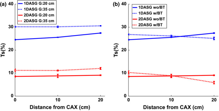
(a) T_S at different air gaps were plotted at all 3 measurement points. (b) T_S measured with and without BT filter. [Color figure can be viewed at wileyonlinelibrary.com]

Table 6.

T_S as a function of air gap at 10 cm from CAX

Air gap (cm)	TS
	1DASG	2DASG
20	25.6 ± 0.1%	8.8 ± 0.7%
35	30.2 ± 0.3%	11.1 ± 0.2%

In contrast with SPR, T_S measured with BT filter did not exhibit large variations across the three measurement points [Fig. 8(b)], and BT filter did not make a large impact on T_S; T_S increased slightly at CAX, and reduced monotonically further away from CAX with BT filter in place. T_S values measured with BT filter were within 1–3% of the values measured without BT filter. 2DASG continued to provide lower Ts values with respect to 1DASG (Table 7).

Table 7.

T_S as a function of BT filter status at 10 and 20 cm from CAX

Measurement location	BT filter status	TS
		1DASG	2DASG
10 cm from CAX	No	25.6 ± 0.1%	8.8 ± 0.7%
10 cm from CAX	Yes	26.2 ± 0.3%	8.9 ± 0.6%
20 cm from CAX	No	27.4 ± 0.1%	9.1 ± 0.1%
20 cm from CAX	Yes	25.1 ± 0.5%	5.9 ± 0.5%

3.D. SNR improvement factor

K_SNR was calculated for all measurement points, and all experiment setups (See Table 1), and it was plotted as a function of SPR without ASG (Fig. 9). Data points were fitted using cubic polynomials to visualize the trends (blue and red lines). When compared to 1DASG, 2DASG provided higher K_SNR values across the range of SPRs investigated in this study, and SNR improvement provided by 2DASG was more emphasized particularly at high SPR conditions. For example, at SPR of 8.7, K_SNR achieved by 1DASG was 1.38, whereas 2DASG provided K_SNR of 2.34, indicating a K_SNR increase by a factor of 1.7 with respect to 1DASG. Change in air gap and presence of BT filter did not make any large difference in K_SNR trends. When SPR was 1.1 or below, K_SNR of 1DASG was less than 1, indicating that SNR was degraded with respect to SNR without ASG. For 2DASG, transition from SNR improvement to SNR degradation occurred (i.e., K_SNR below 1) at SPR of 0.27. At SPR of 0, K_SNR of 1D and 2DASGs were 0.84 and 0.92, respectively, which implies that degradation of SNR was less with 2DASG in the absence of scatter.

Figure 9.

SNR improvement factors, K_SNR , as a function of SPR without ASG. K_SNR were calculated for all measurement points and experiment setups (See Table 1). Cubic polynomials (red and blue lines) were fitted to better visualize trends in K_SNR . [Color figure can be viewed at wileyonlinelibrary.com]

3.E. Low contrast object visualization

Projection images of the contrast phantom are shown in Fig. 10. At a given phantom thickness and detector entrance exposure, all images are displayed at the same gray scale window “width”, whereas gray scale window “level” was set to the mean pixel value of the background in each image. At 20 cm phantom thickness and at both exposure levels, all contrast objects were clearly visible due to relatively high CNR with all grid configurations. At 40 cm phantom thickness, contrast visualization with NOASG was clearly inferior with respect to 1D and 2DASG. When the entrance exposure was reduced from 0.05 mR/frame to 0.025 mR/frame, contrast visualization was lower with all grid configurations, however, 2D ASG still provided better contrast visibility than 1D and NOASG configurations.

Figure 10.

Images of the low contrast phantom for all grid configurations. At each phantom thickness, images were acquired at two different entrance exposures. Images at a given phantom thickness and exposure have the same display window width.

CNR values for the highest contrast object (left most object) are shown in Table 8. At 20 cm phantom thickness, 2D ASG provided at least a factor of 1.3 higher CNR with respect to 1D and NOASG. CNR difference between 1DASG and NOASG was minimal, indicating that the utility of 1DASG in improving CNR was not significant at 20 cm thickness. At 40 cm phantom thickness, CNR provided by 2DASG was at least a factor of 1.9 and 1.4 higher, with respect to NOASG and 1DASG respectively. While CNRs were lower at half the entrance exposure, CNR ratios of different grid configurations were reduced only slightly by the change in exposure levels.

Table 8.

CNRs and CNR ratios for the highest contrast object in Fig. 10

Phantom thickness	Entrance exposure (mR)	CNR			CNR ratios
		NOASG	1DASG	2DASG	1DASG/NOASG	2DASG/NOASG	2DASG/1DASG
20	0.11	14.4 ± 0.5	15.3 ± 0.4	19.9 ± 0.6	1.06	1.38	1.3
20	0.055	10.1 ± 0.4	10.8 ± 0.3	14.0 ± 0.5	1.07	1.39	1.3
40	0.05	2.8 ± 0.2	4.0 ± 0.2	5.6 ± 0.2	1.43	2	1.4
40	0.025	2.1 ± 0.2	2.7 ± 0.2	3.9 ± 0.2	1.3	1.86	1.44

4. Discussion

We developed a 2DASG prototype aimed for CBCT systems in radiation therapy, and evaluated its x‐ray transmission characteristics. As shown in Section 3.A, 2DASG prototype provided about 20% higher primary transmission on the average than the 1DASG installed in the clinical CBCT system. There are multiple factors that explain the higher average primary transmission provided by the 2DASG. First, due to the self‐supporting structure of the 2D grid, interseptal spacers are not needed, whereas fiber spacers used between septa of 1DASG attenuate the primary beam. The second factor is the effect of grid geometry on primary transmission. The 2DASG has a large grid pitch (2.91 mm) with respect to its septal thickness (0.1 mm) which leads to a relatively small footprint on the FPD;⁴⁰ the area covered by the 2DASG's tungsten septa constitutes less than 7% of the FPD's imaging area. On the other hand, 1DASG has a relatively small pitch (0.167 mm) with respect to its septal thickness (0.036 mm), and hence, its footprint covers about 21% of the FPD's imaging area. Another factor that affects primary transmission is the suboptimal geometry and focusing of ASG's septa. Nonuniformities in septal thickness and deviations of septa from ideal focusing geometry increase the shadow of septa in projections, and subsequently, reduce primary transmission. Geometric accuracy of 1D and 2DASGs’ septa cannot be measured directly in projection images (due to the small septal thickness with respect to FPD pixel size), and therefore, its impact on primary transmission was not assessed in this study. However, spatial variations in ASG's geometric accuracy can be evaluated via observing spatial variations in T_P. Standard deviation of T_P was 0.2% and 0.4% for 1D and 2DASGs, respectively, while their mean T_P values were 70.6% (1DASG) and 84.7% (2DASG). Such a small variation in T_P indicates that the geometric accuracy of both ASGs was uniform across the measurement area. While 2DASG provided higher “average” primary transmission, pixel specific primary transmission varied between 32.5% and 99.1% due to the 2DASG's shadow in projections; FPD pixels that were underneath the 2DASG's septa received less primary beam with respect to pixels at the center of grid holes, as visualized in Fig. 4(a). With 1DASG, the variation in pixel specific primary transmission was less than 4%, which was mainly due to its smaller septal pitch with respect to the FPD's pixel pitch. Although, 2DASG provided lower primary transmission to a fraction of pixels, the percentage of such pixels was relatively small (2.8% of FPD pixels received less than 50% primary transmission), and 75% of pixels still received more primary transmission than the maximum pixel specific primary transmission provided by 1DASG.

From scatter suppression point of view, 2DASG provided significantly better performance for all evaluated imaging conditions. When compared to the 1DASG, measured 2DASG SPRs were lower by a factor of 3–6. While both ASGs provided better scatter suppression for larger object thicknesses, 2DASG provided better scatter rejection than 1DASG particularly at larger phantom thicknesses, as indicated by 2DASG's lower T_S values. Engel et al. has also observed and explained this trend in Monte Carlo simulations:⁴¹ At larger object thicknesses, multiple Compton scattered x‐rays constitute a larger percentage of the total scatter intensity, and their angular distribution is broader (i.e., less forward directed).^{6, 41, 42} When compared to 1DASG, a 2DASG is more effective in stopping scattered x‐rays with broader angular distributions due to its septa in two directions. On the other hand, for thinner objects, angular distribution of scatter is more forward directed, and scatter is less likely to be stopped by the 2DASG. While 1DASG is also less effective rejecting forward directed scatter in the direction orthogonal to its septa, its performance in the direction parallel to its septa does not change as a function of object thickness or angular distribution of scatter.

When the air gap was increased from 20 to 35 cm, SPR was reduced for all ASG configurations. Reduction in SPR was due to the relative reduction in scatter intensity, since smaller percentage of scattered x‐rays reaches the FPD as air gap increases.^{7, 39, 43} On the other hand, scatter rejection performance of both ASGs deteriorated at increased air gap, as indicated by the increase in T_S values at 35 cm air gap. This observation is in agreement with other published reports;^{6, 8} as the air gap increases, the angular distribution of scatter is less broad, and scattered radiation is less likely to be stopped by ASG's septa. Hence, T_S increases as air gap increases.

BT filter is often used during imaging of objects with circular or elliptical cross‐sections, and it reduces the spatial variation in exposure incident on the detector. Moreover, BT filter reduces SPR in the central sections (corresponding to thinner BT filter section), and increases SPR in peripheral sections of the reconstructed image (corresponding to thicker BT filter section). Such spatial SPR modulation by BT filter was observed previously with NOASG and 1D ASG configurations.^{5, 12, 44} Our aim in this study was to evaluate whether the use of BT filter in conjunction with 2DASG caused similar spatial variations in SPR. Our observations with NOASG and 1DASG were qualitatively in agreement with the literature.^{5, 13} We observed a similar spatial SPR modulation pattern with 2DASG, albeit it was less emphasized. The effect of BT filter on the scatter suppression performance of 1D and 2DASGs was less pronounced, as indicated by the relatively small difference in T_S values measured with and without BT filter.

Numerous studies have established that reduced scatter fraction in CBCT projections translates into improved CT number accuracy and reduced image artifacts.^{1, 5, 6, 7, 10, 45} Thus, we expect that improved scatter suppression performance of 2DASG is likely to increase the CT number accuracy and reduce scatter‐induced artifacts with respect to CBCT images acquired with 1DASG. Beside improvement in CT number accuracy, another area of interest is the improvement of low contrast resolution. While ASGs reduce scatter intensity, and have a positive effect on improving SNR, they also reduce primary intensity, that deteriorates SNR and contrast resolution. In addition to the transmission characteristics of the ASG, relative intensity of scatter, or SPR, incident on the FPD determines the level of SNR improvement or degradation with the use of ASG. Several studies have reported that conventional 1DASGs reduced SNR and contrast resolution in low to medium scatter intensity environments, where SPR was below 1–2. In our study, SNR degradation with 1DASG (i.e., K_SNR < 1) occurred at SPR values below 1.1, and this result was in agreement with the literature.^{5, 7, 8} Since SPR for various anatomical sites is generally less than two, the role of 1DASGs in SNR improvement is typically limited to high SPR imaging conditions, such as CBCT imaging of pelvis or abdomen.^{5, 6, 7, 8}

Across the SPR range investigated in this study, SNR improvement with 2DASG was higher than 1DASG by a factor of up to 1.7. At higher SPR values, lower scatter transmission by 2DASG plays an important role in SNR improvement, as scatter constitutes a large percentage of the total image signal and noise in projections acquired without ASG. At lower SPR values (e.g., SPR < 1), higher primary transmission by 2DASG becomes a more dominant factor in SNR improvement, as the scatter intensity constitutes a smaller faction of the total x‐ray intensity incident on the FPD. At lower SPR values, SNR improvement by 1DASG is penalized by its lower primary transmission and higher scatter transmission. For example, at 20 cm phantom thickness, SNR improvement by 1DASG was only 1.1 (Fig. 9), whereas 2DASG provided a factor of 1.5 improvement in SNR. For the 1DASG case, the benefit of scatter suppression was almost washed out by the increased noise due to 1DASG's relatively low primary transmission. The role of higher primary transmission is particularly evident at “0” SPR condition, where SNR improvement is solely determined by the primary transmission characteristics of an ASG. At “0” SPR (Fig. 9), K_SNR of 1D and 2DASGs were 0.84 and 0.92 respectively. As a combined effect of both lower scatter and higher primary transmission, 2DASG provided SNR improvement at SPR values down to 0.27. Therefore, the 2DASG may potentially improve contrast resolution in a larger range of SPR conditions with respect to conventional 1DASGs. Improvement in low contrast object visualization and measured CNR improvement factors supported our findings in the SNR improvement study.

Our study employed a 1DASG with a grid ratio of 10, as it was the ASG installed in the clinical TrueBeam CBCT system. While this is a typical grid ratio for commonly utilized 1DASGs, 1DASGs with grid ratios above 15 have been developed in recent years. Such ASGs may provide improved scatter suppression and SNR performance in CBCT imaging. For example, Wiegert et al.⁸ investigated a 1DASG with a grid ratio of 27, and showed that T_S was a factor 2–3 lower with respect to a 1DASG with a grid ratio of 10. However, SNR improvement with high grid ratio was worse, except in high scatter imaging conditions (e.g., SPR > 5), which was attributed to poor primary transmission characteristics of the ASG. Stankovic et al.⁴⁶ employed a 1DASG with grid ratio of 21 in a linac mounted CBCT system. They have shown that both CT number accuracy and contrast to noise ratio (CNR) was improved in a wide range of scatter conditions with respect to CBCT images acquired without ASG. Fetterly and Schueler investigated a similar 1DASG for digital radiography.⁴⁷ They reported a factor 2–3 lower T_S and comparable T_P with respect to 1DASGs with moderate grid ratios, and better SNR improvement in a wide range of scatter conditions. Comparison of 2DASGs with such high grid ratio 1DASGs is an area remains to be investigated.

One of the challenges in implementation of 2DASGs in CBCT is the correction of its septal shadow, or footprint, in projections. If not addressed properly, spatial variations in image intensity may likely to lead to ring artifacts in reconstructed images. Moreover, variations in image intensity may also lead to spatially nonuniform image noise in reconstructions. Similar challenges have been faced in utilization of 2DASGs in breast tomosynthesis,³⁰ and nonlinear grid reciprocation schemes have been implemented to blur the ASG's footprint by moving the ASG at high frequency during x‐ray exposure.⁴⁸ A similar approach was also utilized for crosshatched ASGs in mammography.²⁹ Moreover, image post processing based correction algorithms were developed for 1DASGs that exploit the periodicity of septa footprint to suppress ASG's footprint in projections.^{49, 50, 51} Such post processing approaches may as well be implemented in the context of 2DASGs. Additionally, correction of 2DASG's septal shadow can be further challenged in the presence of gantry flex: As the CBCT gantry rotates, support arms that hold the FPD and x‐ray tube flex, and the position of x‐ray focal point changes in relation to FPD/2DASG assembly during CBCT scan. As a result, the shadow of the 2D ASG projects to different locations in the FPD as a function of gantry rotation. To address this problem, a gantry angle‐specific flat field correction method was developed for 1D ASGs;^{46, 52} since the magnitude and direction of gantry flex is generally reproducible as a function of gantry angle,^{53, 54} each projection of the CBCT scan is flat field corrected by using flat field calibration data previously acquired at a similar gantry angle. We believe that this approach may potentially be employed for 2D ASGs to minimize the grid artifacts introduced by gantry flex.

Another potential concern is the fragility and strength of the 2DASGs. As the grid septa are only 0.1 mm thick, extra care was given during handling of 2DASGs to minimize generation of local stress points on the grid and to reduce the risk of damaging septa. While we have not tested the strength of the prototype, the 2DASG remained intact during routine mounting – dismounting of the grid assembly on the FPD.

Although the proposed 2DASG was aimed toward CBCT applications, 2DASG may also be employed in conventional 2D fluoroscopy to improve low contrast structure visualization. However, several challenges have to be addressed; 2DASG's septa is designed to match the beam divergence for a given fixed source‐detector geometry, whereas in fluoroscopy, source to detector distance (SDD) is often adjusted on a patient specific basis. Varying the SDD will lead to suboptimal alignment of septa with beam divergence, and primary transmission will be further reduced, subsequently reducing potential improvements in CNR. As the shape and intensity of septal shadows will vary as a function of SDD, correction of 2DASG's footprint may be more difficult, or require a different correction approach.

5. Conclusions

A novel prototype 2DASG was developed and its x‐ray transmission properties were evaluated in half‐fan geometry of a linac mounted CBCT system. When compared to a conventional 1DASG, 2DASG reduced SPRs by a factor of 3–6, while providing 19% higher primary transmission on the average. Our results show scatter suppression advantage of 2DASG was maintained at increased air gap and with bow tie filter in place. Lower SPR values achieved with 2DASG may potentially translate into reduced image artifacts and improved CT number accuracy in CBCT. In addition, when compared to 1DASG, 2DASG improved SNR in projections in a wide range of SPRs due to its higher primary transmission and scatter suppression capability. Improved SNR in projection images may lead to improved contrast resolution in CBCT images. While 2DASG exhibited better scatter and primary transmission characteristics, its septal footprint leads to spatially varying primary transmission in projections that may cause artifacts in reconstructed images. 2DASG can be a promising scatter suppression device in improving CBCT image quality in the future with new developed techniques to correct its septal footprint.

References

- 1. Siewerdsen JH, Jaffray DA. Cone‐beam computed tomography with a flat‐panel imager: magnitude and effects of x‐ray scatter. Med Phys. 2001;28:220–231. [DOI] [PubMed] [Google Scholar]
- 2. Ruhrnschopf E‐P, Klingenbeck AK. A general framework and review of scatter correction methods in cone beam CT. Part 2: scatter estimation approaches. Med Phys. 2011;38:5186–5199. [DOI] [PubMed] [Google Scholar]
- 3. Ruhrnschopf EP, Klingenbeck K. A general framework and review of scatter correction methods in x‐ray cone‐beam computerized tomography. Part 1: scatter compensation approaches. Med Phys. 2011;38:4296–4311. [DOI] [PubMed] [Google Scholar]
- 4. Altunbas C. Image corrections for scattered radiation. In: Shaw CC, ed. Cone Beam Computed Tomography. Boca Raton, FL: CRC Press; 2014:129–147. [Google Scholar]
- 5. Lazos D, Williamson JF. Monte Carlo evaluation of scatter mitigation strategies in cone‐beam CT. Med Phys. 2010;37:5456–5470. [DOI] [PMC free article] [PubMed] [Google Scholar]
- 6. Sisniega A, Zbijewski W, Badal A, et al. Monte Carlo study of the effects of system geometry and antiscatter grids on cone‐beam CT scatter distributions. Med Phys. 2013;40:051915. [DOI] [PMC free article] [PubMed] [Google Scholar]
- 7. Kyriakou Y, Kalender W. Efficiency of antiscatter grids for flat‐detector CT. Phys Med Biol. 2007;52:6275–6293. [DOI] [PubMed] [Google Scholar]
- 8. Wiegert J, Bertram M, Schaefer D, et al. Performance of standard fluoroscopy antiscatter grids in flat‐detector‐based cone‐beam CT. Proc SPIE. 2004;5368:67–78. [Google Scholar]
- 9. Siewerdsen JH, Moseley DJ, Bakhtiar B, Richard S, Jaffray DA. The influence of antiscatter grids on soft‐tissue detectability in cone‐beam computed tomography with flat‐panel detectors. Med Phys. 2004;31:3506–3520. [DOI] [PubMed] [Google Scholar]
- 10. Kwan AL, Boone JM, Shah N. Evaluation of x‐ray scatter properties in a dedicated cone‐beam breast CT scanner. Med Phys. 2005;32:2967–2975. [DOI] [PubMed] [Google Scholar]
- 11. Graham SA, Moseley DJ, Siewerdsen JH, Jaffray DA. Compensators for dose and scatter management in cone‐beam computed tomography. Med Phys. 2007;34:2691–2703. [DOI] [PubMed] [Google Scholar]
- 12. Mail N, Moseley DJ, Siewerdsen JH, Jaffray DA. The influence of bowtie filtration on cone‐beam CT image quality. Med Phys. 2009;36:22–32. [DOI] [PubMed] [Google Scholar]
- 13. Menser B, Wiegert J, Wiesner S, Bertram M. Use of beam shapers for cone‐beam CT with off‐centered flat detector. Proc SPIE. 2010;7622:762233. [Google Scholar]
- 14. Ning R, Tang X, Conover DL. X‐ray scatter suppression algorithm for cone‐beam volume CT. Proc SPIE. 2002;4682:774–781. [Google Scholar]
- 15. Sun M, Nagy T, Virshup G, Partain L, Oelhafen M, Star‐Lack J. Correction for patient table‐induced scattered radiation in cone‐beam computed tomography (CBCT). Med Phys. 2011;38:2058–2073. [DOI] [PMC free article] [PubMed] [Google Scholar]
- 16. Zhu L, Bennett NR, Fahrig R. Scatter correction method for X‐ray CT using primary modulation: theory and preliminary results. IEEE Trans Med Imaging. 2006;25:1573–1587. [DOI] [PubMed] [Google Scholar]
- 17. Liu X, Shaw CC, Wang T, Chen L, Altunbas MC, Kappadath SC. An accurate scatter measurement and correction technique for cone beam breast CT imaging using scanning sampled measurement (SSM)technique. Proc SPIE. 2006;6142:614234. [DOI] [PMC free article] [PubMed] [Google Scholar]
- 18. Zbijewski W, Beekman FJ. Efficient Monte Carlo based scatter artifact reduction in cone‐beam micro‐CT. IEEE Trans Med Imaging. 2006;25:817–827. [DOI] [PubMed] [Google Scholar]
- 19. Siewerdsen JH, Daly MJ, Bakhtiar B, et al. A simple, direct method for x‐ray scatter estimation and correction in digital radiography and cone‐beam CT. Med Phys. 2006;33:187–197. [DOI] [PubMed] [Google Scholar]
- 20. Bertram M, Wiegert J, Rose G. Scatter correction for cone‐beam computed tomography using simulated object models. Proc SPIE. 2006;6142:61421C–61421C. [Google Scholar]
- 21. Wiegert J, Hohmann S, Bertram M. Iterative scatter correction based on artifact assessment. Proc SPIE. 2008;6913:69132B. [Google Scholar]
- 22. Poludniowski G, Evans PM, Hansen VN, Webb S. An efficient Monte Carlo‐based algorithm for scatter correction in keV cone‐beam CT. Phys Med Biol. 2009;54:3847–3864. [DOI] [PubMed] [Google Scholar]
- 23. Sechopoulos I. X‐ray scatter correction method for dedicated breast computed tomography. Med Phys. 2012;39:2896–2903. [DOI] [PMC free article] [PubMed] [Google Scholar]
- 24. Altunbas C, Shaw CC, Chen L, et al. A post‐reconstruction method to correct cupping artifacts in cone beam breast computed tomography. Med Phys. 2007;34:3109–3118. [DOI] [PMC free article] [PubMed] [Google Scholar]
- 25. Hatton J, McCurdy B, Greer PB. Cone beam computerized tomography: the effect of calibration of the Hounsfield unit number to electron density on dose calculation accuracy for adaptive radiation therapy. Phys Med Biol. 2009;54:N329. [DOI] [PubMed] [Google Scholar]
- 26. Weiss E, Wu J, Sleeman W, et al. “Clinical evaluation of soft tissue organ boundary visualization on cone‐beam computed tomographic imaging. Int J Radiat Oncol Biol Physics. 2010;78:929–936. [DOI] [PMC free article] [PubMed] [Google Scholar]
- 27. Hou J, Guerrero M, Chen W, D'Souza WD. Deformable planning CT to cone‐beam CT image registration in head‐and‐neck cancer. Med Phys. 2011;38:2088–2094. [DOI] [PubMed] [Google Scholar]
- 28. Landry G, Nijhuis R, Dedes G, et al. Investigating CT to CBCT image registration for head and neck proton therapy as a tool for daily dose recalculation. Med Phys. 2015;42:1354–1366. [DOI] [PubMed] [Google Scholar]
- 29. Makarova OV, Moldovan NA, Tang C‐M, et al. Focused two‐dimensional antiscatter grid for mammography. Proc SPIE. 2002;4783:148–155 [Google Scholar]
- 30. Patel T, Peppard H, Williams MB. Effects on image quality of a 2D antiscatter grid in x‐ray digital breast tomosynthesis: initial experience using the dual modality (x‐ray and molecular) breast tomosynthesis scanner. Med Phys. 2016;43:1720–1735. [DOI] [PMC free article] [PubMed] [Google Scholar]
- 31. Vogtmeier G, Dorscheid R, Engel KJ, et al. Two‐dimensional anti‐scatter grids for computed tomography detectors. Proc SPIE. 2008;6913:691359. [Google Scholar]
- 32. Melnyk R, Boudry J, Liu X, Adamak M. Anti‐scatter grid evaluation for wide‐cone CT. Proc SPIE. 2014;9033:90332P–90337P. [Google Scholar]
- 33. Santos EC, Shiomi M, Osakada K, Laoui T. Rapid manufacturing of metal components by laser forming. Int J Mach Tools Manuf. 2006;46:1459–1468. [Google Scholar]
- 34. Draper NR, Smith H. Applied Regression Analysis. John Wiley & Sons; 2014. [Google Scholar]
- 35. Fetterly KA, Schueler BA. Experimental evaluation of fiber‐interspaced antiscatter grids for large patient imaging with digital x‐ray systems. Phys Med Biol. 2007;52:4863–4880. [DOI] [PubMed] [Google Scholar]
- 36. Lazos D, Williamson JF. Impact of flat panel‐imager veiling glare on scatter‐estimation accuracy and image quality of a commercial on‐board cone‐beam CT imaging system. Med Phys. 2012;39:5639–5651. [DOI] [PMC free article] [PubMed] [Google Scholar]
- 37. Chan HP, Doi K. Investigation of the performance of antiscatter grids: Monte Carlo simulation studies. Phys Med Biol. 1982;27:785–803. [DOI] [PubMed] [Google Scholar]
- 38. Chan HP, Higashida Y, Doi K. Performance of antiscatter grids in diagnostic radiology: experimental measurements and Monte Carlo simulation studies. Med Phys. 1985;12:449–454. [DOI] [PubMed] [Google Scholar]
- 39. Neitzel U. Grids or air gaps for scatter reduction in digital radiography: a model calculation. Med Phys. 1992;19:475–481. [DOI] [PubMed] [Google Scholar]
- 40. Altunbas C, Zhong Y, Shaw C, Kavanagh B, Miften M. SU‐D‐12A‐04: investigation of a 2D Antiscatter Grid for Flat Panel Detectors. Med Phys. 2014;41:124. [Google Scholar]
- 41. Engel KJ, Bäumer C, Wiegert J, Zeitler G. Spectral analysis of scattered radiation in CT. Proc SPIE. 2008;6913:69131R‐69131R‐69111. [Google Scholar]
- 42. Kyriakou Y, Kalender WA. X‐ray scatter data for flat‐panel detector CT. Phys Med Biol. 2007;23:3–15. [DOI] [PubMed] [Google Scholar]
- 43. Persliden J, Carlsson GA. Scatter rejection by air gaps in diagnostic radiology. Calculations using a Monte Carlo collision density method and consideration of molecular interference in coherent scattering. Phys Med Biol. 1997;42:155. [DOI] [PubMed] [Google Scholar]
- 44. Bootsma GJ, Verhaegen F, Jaffray DA. The effects of compensator and imaging geometry on the distribution of x‐ray scatter in CBCT. Med Phys. 2011;38:897–914. [DOI] [PubMed] [Google Scholar]
- 45. Wiegert J, Bertram M. Scattered radiation in flat‐detector based cone‐beam CT: analysis of voxelized patient simulations. Proc SPIE. 2006;6142:614235. [Google Scholar]
- 46. Stankovic U, van Herk M, Ploeger LS, Sonke J‐J. Improved image quality of cone beam CT scans for radiotherapy image guidance using fiber‐interspaced antiscatter grid. Med Phys. 2014;41:061910. [DOI] [PubMed] [Google Scholar]
- 47. Fetterly KA, Schueler BA. Physical evaluation of prototype high‐performance anti‐scatter grids: potential for improved digital radiographic image quality. Phys Med Biol. 2009;54:N37–N42. [DOI] [PubMed] [Google Scholar]
- 48. Patel T, Sporkin H, Peppard H, Williams MB. Design and evaluation of a grid reciprocation scheme for use in digital breast tomosynthesis. Proc SPIE. 2016;978805–978819. [DOI] [PMC free article] [PubMed] [Google Scholar]
- 49. Lin C‐Y, Lee W‐J, Chen S‐J, et al. A study of grid artifacts formation and elimination in computed radiographic images. J Digit Imaging. 2006;19:351–361. [DOI] [PMC free article] [PubMed] [Google Scholar]
- 50. Sasada R, Yamada M, Hara S, Takeo H, Shimura K. Stationary grid pattern removal using 2D technique for moire‐free radiographic image display. Proc SPIE. 2003;688–697. [Google Scholar]
- 51. Tang H, Tong D, Bao XD, Dillenseger J‐L. A new stationary gridline artifact suppression method based on the 2D discrete wavelet transform. Med Phys. 2015;42:1721–1729. [DOI] [PMC free article] [PubMed] [Google Scholar]
- 52. Schafer S, Stayman JW, Zbijewski W, Schmidgunst C, Kleinszig G, Siewerdsen JH. Antiscatter grids in mobile C‐arm cone‐beam CT: effect on image quality and dose. Med Phys. 2012;39:153–159. [DOI] [PMC free article] [PubMed] [Google Scholar]
- 53. Bissonnette JP, Moseley D, White E, Sharpe M, Purdie T, Jaffray DA. Quality assurance for the geometric accuracy of cone‐beam CT guidance in radiation therapy. Int J Radiat Oncol Biol Phys. 2008;71:S57–S61. [DOI] [PubMed] [Google Scholar]
- 54. Sharpe MB, Moseley DJ, Purdie TG, Islam M, Siewerdsen JH, Jaffray DA. The stability of mechanical calibration for a kV cone beam computed tomography system integrated with linear accelerator. Med Phys. 2006;33:136–144. [DOI] [PubMed] [Google Scholar]