Beyond the edge of chaos: Amplification and temporal integration by recurrent networks in the chaotic regime

Abstract

Randomly connected networks of neurons exhibit a transition from fixed-point to chaotic activity as the variance of their synaptic connection strengths is increased. In this study, we analytically evaluate how well a small external input can be reconstructed from a sparse linear readout of network activity. At the transition point, known as the edge of chaos, networks display a number of desirable features, including large gains and integration times. Away from this edge, in the nonchaotic regime that has been the focus of most models and studies, gains and integration times fall off dramatically, which implies that parameters must be fine tuned with considerable precision if high performance is required. Here we show that, near the edge, decoding performance is characterized by a critical exponent that takes a different value on the two sides. As a result, when the network units have an odd saturating nonlinear response function, the falloff in gains and integration times is much slower on the chaotic side of the transition. This means that, under appropriate conditions, good performance can be achieved with less fine tuning beyond the edge, within the chaotic regime.

The dynamic state of a network of neurons influences its information processing capabilities [1]. A network of recurrently connected neurons generates complex dynamics that have been utilized for various computational purposes [2–4]. Large networks of this type exhibit a sharp transition from nonchaotic to chaotic dynamics [5,6], and performance has been characterized as optimal at the edge of this transition [4,7–9]. The location of the transition depends on properties of the inputs to the network [10,11], so maintaining a network right at the edge of chaos would require finely tuning parameters for each input, which is impractical. Therefore, it is important to determine how performance degrades away from this optimal transition point. Here, using a model that is amenable to analytic calculation, we find that, under many circumstances, performance degrades more slowly on the chaotic side of the transition than on the nonchaotic side, showing that it is advantageous to work in the chaotic regime when fine tuning to the edge of chaos cannot be achieved.

Our study is based on a dynamic mean-field calculation applied to randomly connected networks. We compute the signal-to-noise ratio for reconstructing a small external input from a sparse linear readout, a standard network task. This ratio bounds decoding accuracy for both static [12] and dynamic [13] stimuli. To quantify the behavior of the signal-to-noise ratio near the transition point, we evaluate its critical exponents. The analytic expression for the signal-to-noise ratio provides an intuitive picture of the tradeoff between increasing the signal through a larger gain and increasing chaotic noise. The presence of observation noise emphasizes the importance of increasing the signal over decreasing the internally generated noise, providing an advantage to the chaotic state. As outlined above, in the presence of observation noise, the signal-to-noise ratio is maximized at the edge of chaos, where the network time constant shows a critical slowing and small inputs are highly amplified. In addition, at a given distance from the transition point, the chaotic state is often more informative than the nonchaotic state and provides longer-lasting memory.

I. MODEL AND METHOD

We use the dynamic mean-field method [5,10,11,14]to analyze responses of randomly connected networks to external input. For simplicity, we study a discrete-time model with N units. The dynamics of the recurrent input to unit i on trial a (where each trial starts from a different initial condition; what we call trials are also known as replicas) is described by

$$h_i^a(t)={\displaystyle \sum _{j=1}^N{J}_{ij}}{\varphi }_j^a(t),$$ (1)

where J_ij is the coupling strength from unit j to unit i,

$${\varphi }_j^a(t)\equiv \varphi \left(\theta (t-1)+h_j^a(t-1)\right)$$ (2)

is an abbreviation used for a saturating response nonlinearity, ϕ, and θ(t) is a spatially uniform external input. Our goal is to determine how accurately and over what time period θ(t) can be decoded from a linear readout of network activity [15,16]. Each coupling strength is independently and randomly drawn from a distribution with zero mean and standard deviation $g/\sqrt{N}$. For the purposes of calculation, we use a Gaussian distribution, but distributions that include a δ function at zero, corresponding to sparse connections, or that have discrete support, corresponding to a finite number of possible connection strengths, give the same results in the limit of large N.

We introduce a mean-field distribution for the set of state variables $h={\{\mathrm{h}}_i^a(t)\}$ through a Dirac delta function constraint,

$$P(\mathit{h})={\left[{\displaystyle \prod _{i,t,a}\delta \left(h_i^a(t)-{\displaystyle \sum _{j=1}^N{J}_{ij}{\varphi }_j^a(t)}\right)}\right]}_J,$$ (3)

with [·]_J denoting an average over random Gaussian couplings. In the following, we make use of two other averages: E[·| J], which is an average over trials with a fixed {Jij}, and E[·] ≡ [E[·| J ]]_J. In other words, to compute E[·| J], we average over h using the distribution inside the brackets in Eq. (3), removing the average over {Jij}. To compute E[·], we average over h weighted by the full J-averaged distribution of Eq. (3).

Calculations using the dynamic mean-field method [10,14], in the limit of large N, give the moment-generating function for h (see Appendix A),

$$\mathrm{E}\left[\exp \left({\displaystyle \sum _{i,t,a}{\xi }_i^a(t)h_i^a(t)}\right)\right]\approx \exp (Nf(\mathit{\xi },\mathit{q}(\mathit{\xi }),\widehat{\mathit{q}}(\mathit{\xi }))),$$ (4)

where $\mathit{\xi }=\{{\xi }_i^a(t)\}$ is the parameter of the generating function, f is the free energy, and the order parameters q = {q^ab(t,s)} and $\widehat{\mathit{q}}=\{{\widehat{q}}^{ab}\left(t,s\right)\}$ are determined self consistently by the saddle-point equations

$$\frac{\partial f}{\partial \mathit{q}}=0\text{and}\frac{\partial f}{\partial \widehat{\mathit{q}}}=0.$$ (5)

In principle, all the moments of h can be obtained by evaluating the derivatives of the generating function. In particular, the average is $\mathrm{E}[h_i^a(t)]=0$ and the correlation is

$$\mathrm{E}\left[h_i^a(t)h_j^b(s)\right]={\delta }_{ij}{q}^{ab}(t,s).$$ (6)

All higher-order cumulants above the second order are O(1/N).

When the input is constant in time, the system converges to a stationary state. In this case, the self-consistent solution for the order parameter is determined by only two parameters,

$$q^{ab}(t,s)=(q_0-q){\delta }_{ab}{\delta }_{ts}+q,$$ (7)

satisfying, self consistenly,

$$q_0=g^2{\displaystyle \int Dx\varphi {(\theta +\sqrt{q_0}x)}^2},$$ (8)

$$q=g^2{\displaystyle \int DxDy\varphi (\theta +}\sqrt{q_0}x)\varphi \left(\theta +\frac{q}{\sqrt{q_0}}x+\sqrt{\frac{\sqrt{q_0^2}-q^2}{q_0}y}\right)$$

with

$$Dx=\frac{dx{e}^{-x^2/2}}{\sqrt{2\pi }}.$$ (9)

For θ = 0, using a hyperbolic tangent nonlinearity ϕ(x) = tanh(x), q = 0 is a stable solution, so the order parameter simplifies to

$$q^{ab}(t,s)=q_0{\delta }_{ab}{\delta }_{ts},$$ (10)

with q₀ increasing from zero in the chaotic region, g>1 [Fig. 1(a)].

FIG. 1.

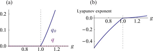
(Color online) The self-consistent solution for the order parameters, q₀ and q (which is 0), in the stationary state (a), and the Lyapunov exponent (b) plotted as a function of the synaptic variability, g. The dotted line at g =1 indicates the edge of chaos.

The chaotic state is characterized by a Lyapunov exponent given in Ref. [10]

$$\frac{1}{2}\ln \int Dx{[\varphi \prime (\theta +\sqrt{q_0}x)]}^2,$$ (11)

which increases more rapidly below the transition to chaos (g<1) than above the transition [g>1; Fig. 1(b)]. This difference foreshadows the asymmetric behavior of the signal detection and integration properties analyzed below, but it is important to point out that our later results do not follow directly from this feature of the Lyapunov exponent. The Lyapunov exponent, which determines how two trajectories starting from nearby initial conditions diverge, and the parameter we use to characterize signal detection and integration measure different things and, depending on the nonlinearity used, can take dissimilar values.

II. SIGNAL-TO-NOISE RATIO

We now evaluate the signal-to-noise ratio for sparse linear decoders designed to optimally read out a dynamic input θ(t) from a fixed subset of K(≪N) units. We assume that the measurement of the total input to network unit i on trial a, $\theta (t)+h_i^a(t)$, is corrupted by Gaussian measurement noise, σ_obsη, of mean zero and variance ${\sigma }_{\text{obs}}^2$, so that the actual measured value is

$$v_i^a(t)=\theta (t)+h_i^a(t)+{\sigma }_{\text{obs}}{\eta }_i^a(t).$$ (12)

We limit our analysis to odd nonlinear functions, ϕ(x)= −ϕ(−x), because this simplifies the analysis. To evaluate the signal-to-noise ratio, we consider a small deviation of the external input from θ = 0 occurring at time t₀. We could alternatively consider decoding information from the nonlinear function of the total input, ϕ(θ + h)+σ_obsη, but the result is unaltered to the leading order for finite σ_obs around the edge of chaos because ϕ(θ + h) ≈ θ + h there.

The average (over networks) signal-to-noise ratio for an optimal linear decoder reading out this perturbation after a measurement period lasting from t₀ to T is [12]

$$R(t_0)\equiv {\displaystyle \sum _{i,j}{{\displaystyle \sum _{t,s⩾t_0}^T\left[\frac{\partial {\mu }_i(t)}{\partial \theta (t_0)}{D}_{ij}(t,s)\frac{\partial {\mu }_j(s)}{\partial \theta (t_0)}\right]}}_J}$$ (13)

where

$${\mu }_i(t)=\mathrm{E}\left[v_i^a(t)|J\right],$$ (14)

and the sums over i and j are restricted to the values of the K units being used in the readout. The quantities in R(t)are all evaluated at θ = 0. The matrix D ≡ C⁻¹ is the inverse of the trial-averaged covariance of the observed K units for a given network (i.e., for a specific {J_ij}), whose elements are described by

$$C_{ij}(t,s)=\text{Cov}\left[v_i^a(t),v_j^a(s)|J\right]=\mathrm{E}\left[(v_i^a(t)-{\mu }_i)(v_j^a(s)-{\mu }_i)|J\right].$$ (15)

It is important for what follows that this covariance matrix has dimensions K×K, not N×N, and that D is the inverse of this K×K matrix.

The memory curve for an optimal linear decoder, which is sometimes used to quantify the ability of networks to buffer past input [15,16], is identical to Eq. (13) for small input. Equation (13) characterizes the accuracy of a readout based on the trial-mean μ. Generally, information could also be readout from higher-order statistics by using nonlinear decoders [12,17,18]. In this sense, Eq. (13) is a lower bound on the information available from more general nonlinear decoders. Note that the optimal linear readout weights depend on the specific {J_ij}, so it is necessary to adjust the decoder for each network.

From the mean-field analysis, we find that each element of the covariance matrix converges to its averaged value in the limit of large N (see Appendix B), i.e.,

$$C_{ij}(t,s)={[C_{ij}(t,s)]}_J+O(N^{-1/2}),$$ (16)

with

$${[C_{ij}(t,s)]}_J={\sigma }_{\text{obs}}^2{\delta }_{ij}{\delta }_{ts}+{\left[\text{Cov}\left[h_i^a(t),h_j^a(s)|J\right]\right]}_J={\delta }_{ij}{\delta }_{ts}\left({\sigma }_{\text{obs}}^2+q_0\right)$$ (17)

evaluated at θ = 0. The O(N^−1/2) term in Eq. (16) introduces corrections of order $\sqrt{K/N}$ into R [Eq. (13)]. To avoid these corrections, we restrict our analysis to the case $K\sim O(\sqrt{N})$. This assures that the O (N^−1/2), J-specific residuals in Eq. (16) do not contribute to R for large N, and we find

$$R(t_0)=\frac{1}{{\sigma }_{\text{obs}}^2+q_0}{\displaystyle \sum _i{{\displaystyle \sum _{t⩾t_0}^T\left[\frac{\partial {\mu }_i(t)}{\partial \theta (t_0)}\frac{\partial {\mu }_i(t)}{\partial \theta (t_0)}\right]}}_J},$$ (18)

with

$${\left[\frac{\partial {\mu }_i(t)}{\partial \theta (t_0)}\frac{\partial {\mu }_i(t)}{\partial \theta (t_0)}\right]}_J={\left[{\frac{{\partial }^2\mathrm{E}\left[v_i^a(t)|J\right]\mathrm{E}\left[v_i^b(t)|J\right]}{\partial {\theta }^a(t_0)\partial {\theta }^b(t_0)}|}_{{\theta }^a={\theta }^b=\theta }\right]}_J={\frac{{\partial }^2\mathrm{E}\left[v_i^a(t)v_i^b(t)\right]}{\partial {\theta }^a(t_0)\partial {\theta }^b(t_0)}|}_{{\theta }^a={\theta }^b=\theta }={\frac{{\partial }^2({\theta }^a(t){\theta }^b(t)+q^{ab}(t,t))}{\partial {\theta }^a(t_0)\partial {\theta }^b(t_0)}|}_{{\theta }^a={\theta }^b=\theta }$$ (19)

for a ≠ b. This means that, to evaluate R, we need to evaluate the second derivative of the order parameter, q. This calculation simplifies for an odd nonlinear response function (see Appendix C), and we obtain

$$R(t_0)=K{\displaystyle \sum _{t⩾t_0}^T\frac{{\gamma }^{t-t_0}}{{\sigma }_{\text{obs}}^2+q_0}}$$ (20)

with

$$\sqrt{\gamma }\equiv g{\displaystyle \int Dx\varphi \prime (\sqrt{q_0}x),}$$ (21)

which corresponds to g times the effective gain (slope) of the response nonlinearity.

Equation (20) tells us that, at any particular time during the measurement period, R receives a contribution from the past input being detected that decays exponentially in time. The decay constant γ therefore determines the memory lifetime of the network, which is −1/ln(γ), and γ near 1 indicates a long memory lifetime. The denominator in Eq. (20) sums two sources of noise, the measurement noise ${\sigma }_{\text{obs}}^2$ and internal network noise quantified by q₀. The best strategy for increasing R is to minimize the internally generated noise, q₀, and to make γ as close to 1 as possible to allow long-time integration of the signal. In the presence of large observation noise σ_obs ≫q₀, the value of R is dominated by how close γ is to 1.

The lifetime variable $\sqrt{\gamma }$ reaches its maximum value γ = 1 at the edge of chaos and, importantly, it decreases more slowly in the chaotic regime than in the nonchaotic regime (Fig. 2). This indicates that, although optimal performance occurs at the edge of chaos and requires fine tuning of g to 1, for a given magnitude of detuning from this value (i.e., a given |g −1|), γ is closer to 1 in the chaotic regime (g> 1; Fig. 2).

FIG. 2.

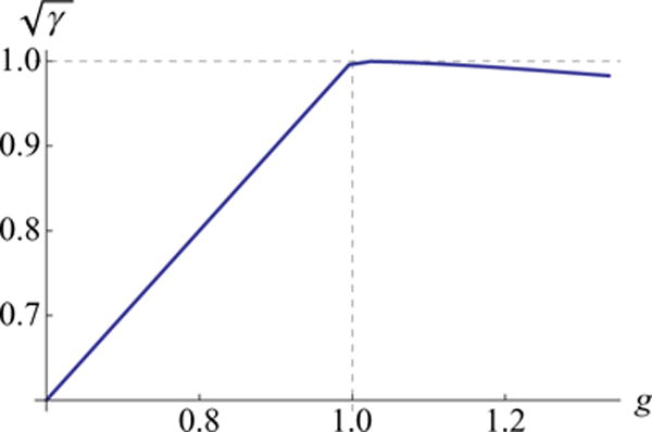
(Color online) The factor $\sqrt{\gamma }$ plotted for ϕ(x) = tanh(x) as a function of the synaptic variability, g. $\sqrt{\gamma }$ takes the maximum value of 1 at the edge of chaos (g = 1; dotted line) and falls off more slowly in the chaotic regime (g>1) than for g<1.

Assuming an infinitely long observation period,

$$R=\frac{K}{{\sigma }_{\text{obs}}^2+q_0}\frac{1}{1-\gamma },$$ (22)

which is plotted as a function of g in Fig. 3 for some σ_obs. When the decay constant γ approaches 1, which happens at the edge of chaos, R diverges because any input perturbations cause perpetually lasting changes in network activity. These analytic results agree well with simulation results (Fig. 4).

FIG. 3.

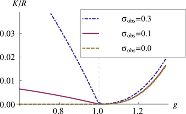
(Color online) The factor K/R plotted for ϕ(x) = tanh(x) as a function of the synaptic variability, g. In the presence of observation noise, R is maximized at the edge of chaos and falls off more slowly in the chaotic regime (g > 1) than for g< 1 reflecting γ shown in Fig. 2.

FIG. 4.

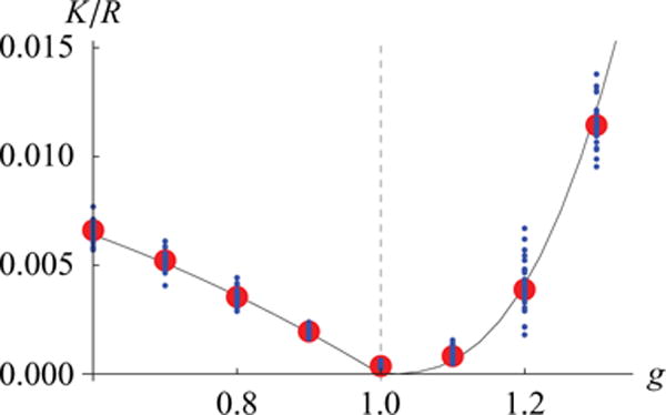
(Color online) Numerical calculation of Eq. (13)(circles) with σ_obs = 0.1. compared with the analytic result of Eq. (22) (solid line). The numerical result was obtained by linearly decoding a simulated network with N = 3000 and K = 20. The small circles describe performances of each network and the large circles describe the average performance across different networks. The analytic results matched well with the numerical results.

III. CRITICAL BEHAVIOR NEAR THE EDGE OF CHAOS

We next analyze the critical behavior of the system near the edge of chaos. By definition, the derivative of ϕ at 0 is 1, so we can expand any odd, monotonically increasing ϕ as

$$\varphi (x)=x+\frac{{\alpha }_3{x}^3}{3!}+\frac{{\alpha }_5{x}^5}{5!}+\cdots .$$ (23)

The Landau expansion of Eq. (8) for small q₀ yields that the sign of α₃ determines the nature of the phase transition around q₀ = 0. The system shows a first-order transition if the nonlinearity is accelerating (α₃ > 0). In this case, q₀ jumps discontinuously from zero to a positive value at g = 1 as g increases. The transition is second order if the nonlinearity is saturating (α₃ < 0). In this case, q₀ increases from zero continuously at g = 1 as g increases. The analysis of the critical behavior is much easier for the second-order transition (α₃ < 0), the case we examine.

We analyze the critical behavior of R near the edge of chaos, that is, for small Δg≡g −1, using Eqs. (20) and (21). In the nonchaotic regime (Δg < 0), q₀ = 0 so the decay factor is γ = g². From Eq. (22), we find that

$$R=\frac{K}{{\sigma }_{\text{obs}}^2(1-g^2)}\approx \frac{K}{2{\sigma }_{\text{obs}}^2|\mathrm{\Delta }g|}.$$ (24)

In the chaotic regime (Δg > 0), we expand Eq. (8) for small q₀ and find that the order parameter is

$$q_0=\frac{2}{|{\alpha }_3|}\mathrm{\Delta }g+\frac{{\alpha }_5/{\alpha }_3^2-4/3}{|{\alpha }_3|}\mathrm{\Delta }{g}^2+O(\mathrm{\Delta }{g}^3).$$ (25)

Based on this expression, the effective gain is $\sqrt{\gamma }\approx 1-\mathrm{\Delta }{g}^2/3$ to leading order. Hence, to leading order,

$$R=\frac{3K}{2{\sigma }_{\text{obs}}^2{(\mathrm{\Delta }g)}^2}$$ (26)

near the edge but on the chaotic side. Interestingly, the dependencies of $\sqrt{\gamma }$ and R on ϕ (such as α₃ and α₅) disappear up to this order. In contrast to the nonchaotic regime with R ~ Δg⁻¹, the divergence is stronger in the chaotic regime with R ~ Δg⁻², yielding larger R at an equal distance, |Δg|, away from the edge (Fig. 5).

FIG. 5.

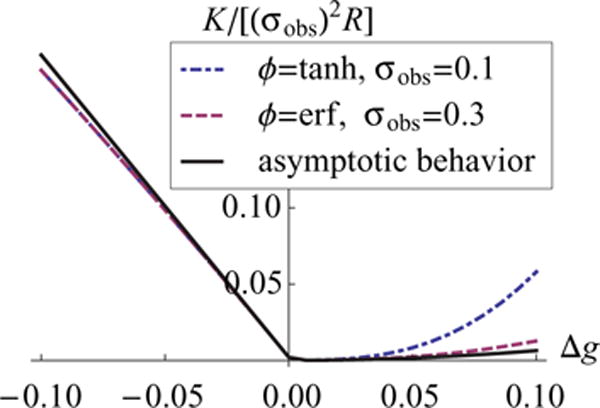
(Color online) The critical behavior of R does not depend on details of the nonlinearity or on the noise level. For any saturating odd nonlinear response function, R diverges linearly on the nonchaotic and quadratically on the chaotic side of the edge or transition. The solid line describes the asymptotic behavior; the dash-dotted line describes ϕ(x) = tanh(x) and σ_obs = 0.1; and the dashed line describes $\varphi (x)=\text{erf}(\sqrt{\pi }x/2)$ and σ_obs = 0.3.

We have determined analytically that the signal-to-noise ratio of large randomly connected networks diverges at the edge of chaos, and the memory lifetime of the network also diverges. Observation noise is an important element for this property. Without observation noise, any network without internally generated noise yields an infinite R. On the other hand, addition of observation noise emphasizes the benefit of increasing signal over increasing internally generated noise. Hence, if a deterministic network performs sensory or memory processing and if a receiver of its output has limited observational resolution, it is advantageous to increase the signal by increasing the network gain. Generally, setting network parameters right at the edge of chaos requires fine tuning. We have shown that at the same small distance away from the edge, R is larger in the chaotic regime than in the nonchaotic regime for any saturating odd nonlinear function.

Although, we have concentrated on a rather special situation in this paper for mathematical simplicity, several lines of generalization are possible without losing analytic tractability. First, we have neglected internal stochastic noise within the network. Although neurons behave irregularly in networks, they respond reliably in isolation. This observation has lead to a speculation that the dominant apparent stochasticity of cortical circuits is generated by the chaotic dynamics of, individually, essentially deterministic neurons [6]. The mean-field analysis with system noise has been studied previously [10]. With an addition of small system noise, R is peaked (but does not diverge) near the edge of chaos on the nonchaotic side. Second, we have concentrated on a class of odd nonlinear response functions. This assumption is a mathematical convenience that simplifies the final expression of R. For a general response nonlinearity, R depends not only on γ and q₀ but on other factors as well. Third, although we considered discrete temporal dynamics, it is possible to analyze a continuous-time model in a similar way [5,11]. We believe that qualitative aspects of the signal-to-noise ratio are common in the two models. Fourth, although we consider unstructured networks in this paper, it would be interesting to study how structured connections change chaotic dynamics [19] and influence signal extraction and integration [20].

APPENDIX A: MEAN-FIELD CALCULATION

In this appendix, we calculate the moment-generating function of Eq. (4). We denote $h_i^a(t)=h_{it}^a$ and $\varphi (\theta (t-1)+h_j^a(t-1))={\varphi }_{jt}^a$. In this section, we follow the convention that summation is implied when the same index appear twice in an expression (e.g., ${\displaystyle {\sum }_j{J}_{ij}{\varphi }_{jt}^a=J_{ij}{\varphi }_{jt}^a}$). A calculation of the moment-generating function (as a function of ξ) yields

$$Z(\mathbf{\xi })={\left[{\displaystyle \int \left(\prod _{i,t,a}d{h}_{it}^a\right)}\exp \left({\xi }_{it}^a{h}_{it}^a\right)\prod _{i,t,a}\delta \left(h_{it}^a-J_{ij}{\varphi }_{jt}^a\right)\right]}_J={\displaystyle \int dH}\exp \left({\xi }_{it}^a{h}_{it}^a+\mathrm{i}{\widehat{h}}_{it}^a{h}_{it}^a\right){\left[\exp \left(-\mathrm{i}{\widehat{h}}_{it}^a{\varphi }_{jt}^a{J}_{ij}\right)\right]}_J={\displaystyle \int dH}\exp \left({\xi }_{it}^a{h}_{it}^a+\mathrm{i}{\widehat{h}}_{it}^a{h}_{it}^a+\frac{g^2}{2N}\mathrm{i}{\widehat{h}}_{it}^a\mathrm{i}{\widehat{h}}_{is}^b{\varphi }_{jt}^a{\varphi }_{js}^b\right)={\displaystyle \int dH}\left({\displaystyle \int \prod _{t,s,a,b}}Nd{q}_{ts}^{ab}\delta (N{q}_{ts}^{ab}-g^2{\varphi }_{jt}^a{\varphi }_{js}^b)\right)\exp \left({\xi }_{it}^a{h}_{it}^a+\mathrm{i}{\widehat{h}}_{it}^a{h}_{it}^a+\frac{1}{2}{q}_{ts}^{ab}\mathrm{i}{\widehat{h}}_{it}^a\mathrm{i}{\widehat{h}}_{is}^b\right)={\displaystyle \int \left(\prod _{t,s,a,b}\frac{Nd{q}_{ts}^{ab}d{\widehat{q}}_{ts}^{ab}}{2\pi }\right){\displaystyle \int dH}\exp (\mathrm{i}{\widehat{q}}_{ts}^{ab}(N{q}_{ts}^{ab}-g^2{\varphi }_{jt}^a{\varphi }_{js}^b)+}{\xi }_{it}^a{h}_{it}^a+\mathrm{i}{\widehat{h}}_{it}^a{h}_{it}^a+\frac{1}{2}{q}_{ts}^{ab}\mathrm{i}{\widehat{h}}_{it}^a\mathrm{i}{\widehat{h}}_{is}^b)={\displaystyle \int \left(\prod _{t,s,a,b}\frac{Nd{q}_{ts}^{ab}d{\widehat{q}}_{ts}^{ab}}{2\pi }\right)}\exp (Nf(\mathit{\xi },\mathit{q},\widehat{\mathit{q}})),$$ (A1)

where $dH\equiv {\mathrm{\Pi }}_{i,t,a}(d{h}_{it}^{a}d{\widehat{h}}_{it}^a/2\pi )$,

$$f(\mathit{\xi },\mathit{q},\widehat{\mathit{q}})\equiv \mathrm{i}{\widehat{q}}_{ts}^{ab}{q}_{ts}^{ab}+\frac{1}{N}\log {\displaystyle \int e^{ℒ}dH},$$ (A2)

and

$$ℒ\equiv {\xi }_{it}^a{h}_{it}^a+\mathrm{i}{\widehat{h}}_{it}^a{h}_{it}^a+\frac{1}{2}{q}_{ts}^{ab}\mathrm{i}{\widehat{h}}_{it}^a\mathrm{i}{\widehat{h}}_{is}^b-g^2\mathrm{i}{\widehat{q}}_{ts}^{ab}{\varphi }_{it}^a{\varphi }_{is}^b.$$ (A3)

Next, we use the saddle-point method to evaluate Z(ξ). To leading order, the integrals of q and $\widehat{q}$ are approximated by the saddle-point value, i.e.,

$$\ln Z(\mathit{\xi })\approx Nf(\mathit{\xi },\mathit{q}(\mathit{\xi }),\widehat{\mathit{q}}(\mathit{\xi })),$$ (A4)

and the saddle-point, [q(ξ), $\widehat{\mathit{q}}\left(\mathit{\xi }\right)$], is determined self consistently by solving

$$0=\frac{\partial f}{\partial q_{ts}^{ab}}=\mathrm{i}{\widehat{q}}_{ts}^{ab}+\frac{1}{2N}{\langle \mathrm{i}{\widehat{h}}_{it}^a\mathrm{i}{\widehat{h}}_{is}^b\rangle }_{ℒ},0=\frac{\partial f}{\partial \mathrm{i}{\widehat{q}}_{ts}^{ab}}=q_{ts}^{ab}-\frac{g^2}{N}{\langle {\varphi }_{it}^a{\varphi }_{is}^b\rangle }_{ℒ},$$ (A5)

with the average, 〈·〉_ℒ, defined as

$${\langle A\rangle }_{ℒ}\equiv \frac{\int A{e}^{ℒ}dH}{\int e^{ℒ}dH}.$$ (A6)

Equation (A5) is especially easy to solve when ξ = 0 because $\widehat{\mathit{q}}\left(0\right)=0$ is a self-consistent solution of Eq. (A5). To confirm this, we define ${ℒ}_0\equiv ℒ{|}_{\xi =0,\widehat{q}=0}=\mathrm{i}{\widehat{h}}_{it}^a{h}_{it}^a+q_{ts}^{ab}(0)\mathrm{i}{\widehat{h}}_{it}^a\mathrm{i}{\widehat{h}}_{is}^b/2$, and find that

$${\langle \mathrm{i}{\widehat{h}}_{it}^a\mathrm{i}{\widehat{h}}_{is}^b\rangle }_{{ℒ}_0}=2\frac{\partial }{\partial q_{ts}^{ab}}{\displaystyle \int e^{{ℒ}_0}dH=0.}$$ (A7)

Hence, when ξ = 0, a solution of the saddle-point condition is

$$q_{ts}^{ab}=g^2{\displaystyle \int \left(\frac{{\prod }_{t,a}d{h}_t^a}{\sqrt{\det (2\pi q)}}\right)}{\varphi }_t^a{\varphi }_s^b\exp \left(-\frac{1}{2}{(q^{-1})}_{ts}^{ab}{h}_t^a{h}_s^b\right),$$

$${\widehat{q}}_{ts}^{ab}=0.$$ (A8)

Note that, in the above expression, ${\langle \cdot \rangle }_{{ℒ}_0}$ describes a Gaussian average of h with mean zero and covariance ${\delta }_{ij}{q}_{ts}^{ab}$. The possibility of a $\widehat{\mathit{q}}\left(0\right)\ne 0$ solution is not within the scope of this paper (see Ref. [14], for example). Thus, we concentrate on the $\widehat{\mathit{q}}\left(0\right)=0$ solution Eq. (A8) in the following.

In principal, we can obtain all higher-order cumulants of h by differentiating the cumulant-generating function ln Z(ξ) = Nf (ξ,q(ξ), $\widehat{\mathit{q}}(\mathit{\xi }))$ by ξ and, then, setting ξ = 0. From the normalization constraint, ln Z(0) = 0. The first derivative is

$$N\frac{df}{d{\xi }_{it}^a}=N\frac{\partial f}{\partial {\xi }_{it}^a}+N\frac{\partial f}{\partial \mathit{q}}\frac{\partial \mathit{q}}{\partial {\xi }_{it}^a}+N\frac{\partial f}{\partial \widehat{\mathit{q}}}\frac{\partial \widehat{\mathit{q}}}{\partial {\xi }_{it}^a}=N\frac{\partial f}{\partial {\xi }_{it}^a},$$ (A9)

because ∂f/∂q = 0 and $\partial f/\partial \widehat{\mathit{q}}=0$ at the saddle-point Eq. (A5). Hence, the first-order cumulant is

$${\mathrm{E}\left[h_{it}^a\right]\approx N\frac{\partial f}{\partial {\xi }_{it}^a}|}_{\xi =0}={\langle h_{it}^a\rangle }_{{ℒ}_0}=0.$$ (A10)

The calculation of high-order cumulants becomes easier if we neglect O(1/N) factors. First, ${{\partial }^{n}f/\partial \mathit{\xi }}^n=O(1/N)$ for n ⩾ 1 at ξ = 0. Moreover, the nth (n ⩾ 1) derivatives of the order parameters are ${{\partial }^n\mathit{q}/\partial \mathit{\xi }}^n=O(1/N)$ and ${{\partial }^n\widehat{\mathit{q}}/\partial \mathit{\xi }}^n=O(1/N)$ at ξ = 0 from Eq. (A5). This means that perturbations to a single unit contribute only ~1/N to the mean-field variables, which are defined by averaging over N units. Hence, terms that contain derivatives of order parameters contribute only to O (1 /N) terms. Thus, for the calculation of higher-order cumulants, the full derivatives of ξ can be approximated by its partial derivatives, d/dξ ≈ ∂/∂ξ, and the order parameters can be approximated, using their ξ = 0 values as q(ξ) ≈ q(0) and $\widehat{q}\left(\xi \right)\approx \widehat{q}\left(0\right)$. Neglecting O(1/N) terms, we find

$$Nf(\mathit{\xi },\mathit{q}(0)\widehat{\mathit{q}}(0))=\text{ln}{\displaystyle \int \mathit{dH}\exp \left({\xi }_{it}^a{h}_{it}^a+\mathrm{i}{\widehat{h}}_{it}^a{h}_{it}^a+\frac{1}{2}{q}_{ts}^{ab}(0)\mathrm{i}{\widehat{h}}_{it}^a\mathrm{i}{\widehat{h}}_{is}^b\right)}=\frac{1}{2}{q}_{ts}^{ab}(0){\xi }_{it}^a{\xi }_{is}^b.$$ (A11)

This shows that the mean-field distribution P(h) is a Gaussian distribution for independent units with mean zero and covariance ${\delta }_{ij}{q}_{ts}^{ab}(0)$ up to O(1/N) terms. Hence, to this precision, the two averages E[·] and ${\langle \cdot \rangle }_{{ℒ}_0}$ are indistinguishable.

APPENDIX B: NETWORK SPECIFIC STATISTICS

In this appendix, we evaluate statistics of the state variable, h, for given {J_ij}. The trial-mean of a quantity A(h) is written as E[A(h)| J], where each trial has different initial conditions at t→ −∞. When the system is ergodic this trial average does not depend on a specific set of initial conditions. From this definition and Eq. (A11), to the leading order, we can derive the following:

$${[\mathrm{E}[h_{it}|J]]}_J=\mathrm{E}[h_{it}]=O(1/N)\text{and}{[\text{Cov}[h_{it},h_{js}|J]]}_J=[\mathrm{E}{[h_{it}{h}_{js}|J]-\mathrm{E}[h_{it}|J]\mathrm{E}[h_{js}|J]]}_J=[\mathrm{E}{[h_{it}^a{h}_{js}^a|J]-\mathrm{E}[h_{it}^a{h}_{js}^b|J]]}_J=\mathrm{E}[h_{it}^a{h}_{js}^a]-\mathrm{E}[h_{it}^a{h}_{js}^b]={\delta }_{ij}(q_{ts}^S-q_{ts}^D)+O(1/N),$$ (B1)

where a ≠ b, and $q_{ts}^{aa}=q_{ts}^S$ and $q_{ts}^{ab}=q_{ts}^D$. Now we define the network specific covariance as Γ_ij;ts ≡ Cov[h_it,h_js|J] and evaluate how Γ is different from one realization of {J_ij} to another. The variance of Γ across networks is, from Eq. (A11),

$${[{\mathrm{\Gamma }}_{ij;ts}^2]}_J-{[{\mathrm{\Gamma }}_{ij;ts}]}_J^2=[(\mathrm{E}[h_{it}^a{h}_{js}^a|J]-{{\mathrm{E}[h_{it}^a{h}_{js}^b|J])}^2]}_J-(\mathrm{E}[h_{it}^a{h}_{js}^a]-{\mathrm{E}[h_{it}^a{h}_{js}^b])}^2=\mathrm{E}[h_{it}^a{h}_{js}^a{h}_{it}^c{h}_{js}^c]-2\mathrm{E}[h_{it}^a{h}_{js}^a{h}_{it}^c{h}_{js}^d]+\mathrm{E}[h_{it}^a{h}_{js}^b{h}_{it}^c{h}_{js}^d]+{(\mathrm{E}[h_{it}^a{h}_{js}^a]-\mathrm{E}[h_{it}^a{h}_{js}^b])}^2={\delta }_{ij}\{(q_{ts}^S{q}_{ts}^S+q_{ts}^D{q}_{ts}^D+q_{tt}^D{q}_{ss}^D)-2(q_{ts}^S{q}_{ts}^D+q_{ts}^D{q}_{ts}^D+q_{tt}^D{q}_{ss}^D)+(2q_{ts}^D{q}_{ts}^D+q_{tt}^D{q}_{ss}^D)-{(q_{ts}^S{q}_{ts}^D)}^2\}\times (1-{\delta }_{ij})\{q_{tt}^D{q}_{ss}^D-2q_{tt}^D{q}_{ss}^D+q_{tt}^D{q}_{ss}^D\}+O(1/N)=O(1/N),$$ (B2)

where a,b,c,d are all different. Therefore, each component of Γ converges to its network average as

$${\mathrm{\Gamma }}_{ij;ts}={[{\mathrm{\Gamma }}_{ij;ts}]}_J+O(N^{-1/2}).$$ (B3)

APPENDIX C: PERTURBATION EXPANSION OF THE ORDER PARAMETER

In this appendix, we evaluate the signal component of Eq. (19) by calculating the responses of the order parameter, $\left\{q_{tt}^{ab}\right\}$, to perturbations in the external input, $\mathit{\theta }=\left\{{\theta }_t^a\right\}$. Dynamic evolution of the order parameter is described by the saddle-point Eq. (A8), which we repeat here for convenience

$$q_{t+1,t+1}^{ab}=g^2{\langle {\varphi }_{t+1}^a{\varphi }_{t+1}^b\rangle }_{{ℒ}_0}=g^2{\displaystyle \int \left(\frac{{\mathrm{\Pi }}_{t,a}d{h}_t^a}{\sqrt{\det (2\pi q)}}\right)}\varphi \left({\theta }_t^a+h_t^a\right)\varphi \left({\theta }_t^b+h_t^b\right)\exp \left(-\frac{1}{2}{(q^{-1})}_{ts}^{ab}{h}_t^a{h}_s^b\right),$$

where ${ℒ}_0\equiv ℒ{|}_{\xi =0,\widehat{q}=0}$. To simplify expressions, we omit the temporal index so that ${\theta }_t^a={\theta }^a$ and $q_{tt}^{ab}=q^{ab}$ in the following, and find that, for general smooth functions ϕ and ѱ, the Gaussian integral is expressed as

$${\langle {\varphi }^a{\psi }^b\rangle }_{{ℒ}_0}\equiv {\langle \varphi \left({\theta }_t^a+h_t^a\right)\psi \left({\theta }_t^b+h_t^b\right)\rangle }_{{ℒ}_0}={\displaystyle \int DxDy\varphi ({\theta }^a+\sqrt{q^{aa}}x)\psi \left({\theta }^b+\frac{q^{ab}}{\sqrt{q^{aa}}}x+\sqrt{\frac{q^{aa}{q}^{bb}-{(q^{ab})}^2}{q^{aa}}}y\right)},$$ (C1)

with $Dx\equiv dx{e}^{-x^2/2}/\sqrt{2\pi }$. Note that this expression implies that h^a and h^b have variances of q^aa and q^bb, respectively, and covariance q^ab under the average, ${\langle \cdot \rangle }_{{ℒ}_0}$. The first derivative of this average is

$$d{\langle {\varphi }^a{\psi }^b\rangle }_{{ℒ}_0}={\langle {{\varphi }^{\prime }}^a{\psi }^b\rangle }_{{ℒ}_0}d{\theta }^a+{\langle {\varphi }^a{{\psi }^{\prime }}^b\rangle }_{{ℒ}_0}d{\theta }^b+\frac{1}{2}\left(\frac{1}{\sqrt{q^{aa}}}{\langle x{{\varphi }^{\prime }}^a{\psi }^b\rangle }_{{ℒ}_0}-\frac{q^{ab}}{{\sqrt{q^{aa}}}^3}{\langle x{\varphi }^a{{\psi }^{\prime }}^b\rangle }_{{ℒ}_0}+\frac{{\left(\frac{q^{ab}}{q^{aa}}\right)}^2}{\sqrt{\frac{q^{aa}{q}^{bb}-{\left(q^{ab}\right)}^2}{q^{aa}}}}{\langle y{\varphi }^a{{\psi }^{\prime }}^b\rangle }_{{ℒ}_0}\right)d{q}^{aa}+\frac{1}{2\sqrt{\frac{q^{aa}{q}^{bb}-{\left(q^{ab}\right)}^2}{q^{aa}}}}{\langle y{\varphi }^a{{\psi }^{\prime }}^b\rangle }_{{ℒ}_0}d{q}^{bb}+\left(\frac{1}{\sqrt{q^{aa}}}{\langle x{\varphi }^a{{\psi }^{\prime }}^b\rangle }_{{ℒ}_0}+\frac{-\frac{q^{ab}}{q^{aa}}}{\sqrt{\frac{q^{aa}{q}^{bb}-{\left(q^{ab}\right)}^2}{q^{aa}}}}{\langle y{\varphi }^a{{\psi }^{\prime }}^b\rangle }_{{ℒ}_0}\right)d{q}^{ab}={\overrightarrow{a}}^{T}d\overrightarrow{\mathrm{\Theta }}$$ (C2)

with vectors $\overrightarrow{a}={({\langle {{\varphi }^{\prime }}^a{\psi }^b\rangle }_{{ℒ}_0},{\langle {\varphi }^a{{\psi }^{\prime }}^b\rangle }_{{ℒ}_0},{\langle {{\varphi }^{″}}^a{\psi }^b\rangle }_{{ℒ}_0},{\langle {\varphi }^a{{\psi }^{″}}^b\rangle }_{{ℒ}_0},{\langle {{\varphi }^{\prime }}^a{{\psi }^{\prime }}^b\rangle }_{{ℒ}_0})}^T$ and $\overrightarrow{\mathrm{\Theta }}={({\theta }^a,{\theta }^b,q^{aa}/2,q^{bb}/2,q^{ab})}^T$.

In the second line of Eq. (C2), we used the following relations

$${\langle x{\varphi }^a{\psi }^b\rangle }_{{ℒ}_0}={\langle \left(\frac{d}{dx}{\varphi }^a{\psi }^b\right)\rangle }_{{ℒ}_0}=\sqrt{q^{aa}}{\langle {{\varphi }^{\prime }}^a{\psi }^b\rangle }_{{ℒ}_0}+\frac{q^{ab}}{\sqrt{q^{aa}}}{\langle {\varphi }^a{{\psi }^{\prime }}^b\rangle }_{{ℒ}_0},$$ (C3)

$${\langle y{\varphi }^a{\psi }^b\rangle }_{{ℒ}_0}={\langle \left(\frac{d}{dy}{\varphi }^a{\psi }^b\right)\rangle }_{{ℒ}_0}=\sqrt{\frac{q^{aa}{q}^{bb}-{(q^{ab})}^2}{q^{aa}}}{\langle {\varphi }^a{{\psi }^{\prime }}^b\rangle }_{{ℒ}_0},$$ (C4)

obtained from integration by parts. Similarly, using Eq. (C2) repeatedly, the second derivative is

$$d^2{\langle {\varphi }^a{\psi }^b\rangle }_{{ℒ}_0}={\overrightarrow{a}}^T{d}^2\overrightarrow{\mathrm{\Theta }}+{(d\overrightarrow{\mathrm{\Theta }})}^{T}d\overrightarrow{a}={\overrightarrow{a}}^T{d}^2\overrightarrow{\mathrm{\Theta }}+{(d\overrightarrow{\mathrm{\Theta }})}^{T}Ad\overrightarrow{\mathrm{\Theta }},$$ (C5)

where, applying Eq. (C2) once again to each component of $\overrightarrow{a}$, we find $d\overrightarrow{a}=Ad\overrightarrow{\mathrm{\Theta }}$ with

$$A=\left(\begin{array}{ccccc}{\langle {{\varphi }^{″}}^a{\psi }^b\rangle }_{{ℒ}_0}& {\langle {{\varphi }^{\prime }}^a{{\psi }^{\prime }}^b\rangle }_{{ℒ}_0}& {\langle {{{\varphi }^{\prime }}^{″}}^a{\psi }^b\rangle }_{{ℒ}_0}& {\langle {{\varphi }^{\prime }}^a{{\psi }^{″}}^b\rangle }_{{ℒ}_0}& {\langle {{\varphi }^{″}}^a{{\psi }^{\prime }}^b\rangle }_{{ℒ}_0}\\ {\langle {{\varphi }^{\prime }}^a{{\psi }^{\prime }}^b\rangle }_{{ℒ}_0}& {\langle {\varphi }^a{{\psi }^{″}}^b\rangle }_{{ℒ}_0}& {\langle {{\varphi }^{″}}^a{{\psi }^{\prime }}^b\rangle }_{{ℒ}_0}& {\langle {\varphi }^a{{{\psi }^{\prime }}^{″}}^b\rangle }_{{ℒ}_0}& {\langle {{\varphi }^{\prime }}^a{{\psi }^{″}}^b\rangle }_{{ℒ}_0}\\ {\langle {{{\varphi }^{\prime }}^{″}}^a{\psi }^b\rangle }_{{ℒ}_0}& {\langle {{\varphi }^{″}}^a{{\psi }^{\prime }}^b\rangle }_{{ℒ}_0}& {\langle {{{\varphi }^{″}}^{″}}^a{\psi }^b\rangle }_{{ℒ}_0}& {\langle {{\varphi }^{″}}^a{{\psi }^{″}}^b\rangle }_{{ℒ}_0}& {\langle {{{\varphi }^{\prime }}^{″}}^a{{\psi }^{\prime }}^b\rangle }_{{ℒ}_0}\\ {\langle {{\varphi }^{\prime }}^a{{\psi }^{″}}^b\rangle }_{{ℒ}_0}& {\langle {\varphi }^a{{{\psi }^{\prime }}^{″}}^b\rangle }_{{ℒ}_0}& {\langle {{\varphi }^{″}}^a{{\psi }^{″}}^b\rangle }_{{ℒ}_0}& {\langle {\varphi }^a{{{\psi }^{″}}^{″}}^b\rangle }_{{ℒ}_0}& {\langle {{\varphi }^{\prime }}^a{{{\psi }^{\prime }}^{″}}^b\rangle }_{{ℒ}_0}\\ {\langle {{\varphi }^{″}}^a{{\psi }^{\prime }}^b\rangle }_{{ℒ}_0}& {\langle {{\varphi }^{\prime }}^a{{\psi }^{″}}^b\rangle }_{{ℒ}_0}& {\langle {{{\varphi }^{\prime }}^{″}}^a{{\psi }^{\prime }}^b\rangle }_{{ℒ}_0}& {\langle {{\varphi }^{\prime }}^a{{{\psi }^{\prime }}^{″}}^b\rangle }_{{ℒ}_0}& {\langle {{\varphi }^{″}}^a{{\psi }^{″}}^b\rangle }_{{ℒ}_0}\end{array}\right).$$ (C6)

Although we had to distinguish ϕ and ψ to derive Eq. (C5), we only have to consider the derivatives of ${\langle {\varphi }^a{\varphi }^b\rangle }_{{ℒ}_0}$ in the following, so we can replace ψ by ϕ. When the external input is constant in time, the order parameter takes only two distinctive values, $q_{ts}^{ab}=(q_0-q){\delta }_{ab}{\delta }_{ts}+q$ in the stationary state [see Eq. (7)]. Moreover, when the response nonlinearity is an odd function and the input is zero, θ = 0, we know that q = 0 is a stable solution. Hence, in this case, it is easy to check that

$${\langle {\varphi }^{(m)}(h^a){\varphi }^{(n)}(h^b)\rangle }_{{ℒ}_0}=0\text{if}m+n\text{is}\text{odd}$$ (C7)

for all integers m and n, where ϕ⁽ⁿ⁾ is the nth derivative of ϕ. When θ = 0, the order parameter q^ab = 0 for a ≠ b, meaning that h^a and h^b are independent Gaussian random variables of mean zero. In this case, Eq. (C7) results because either ϕ^(m) or ϕ⁽ⁿ⁾ (with an even m or n) is an odd function. When a = b, on the other hand, ϕ^(m)(h^a)ϕ⁽ⁿ⁾(h^a) is an odd function of a Gaussian random variable, h^a with zero mean. Using Eq. (C7), Eq. (C2) can be simplified to

$$d{\langle {\varphi }^a{\varphi }^b\rangle }_{{ℒ}_0}={\langle {{\varphi }^{″}}^a{\varphi }^b\rangle }_{{ℒ}_0}\frac{d{q}^{aa}}{2}+{\langle {\varphi }^a{{\varphi }^{″}}^b\rangle }_{{ℒ}_0}\frac{d{q}^{bb}}{2}+{\langle {{\varphi }^{\prime }}^a{\varphi }^b\rangle }_{{ℒ}_0}{\mathit{dq}}^{ab}.$$ (C8)

Because $q_{t+1,t+1}^{ab}=g^2{\langle {\varphi }^a{\varphi }^b\rangle }_{{ℒ}_0}$, we obtain the self-consistent update equations

$$d{q}_{t+1,t+1}^{aa}=g^2({\langle {\varphi }^a{{\varphi }^{″}}^a\rangle }_{{ℒ}_0}+{\langle {{\varphi }^{\prime }}^a{{\varphi }^{\prime }}^a\rangle }_{{ℒ}_0})d{q}_{tt}^{aa}$$ (C9)

when a = b, and

$$d{q}_{t+1,t+1}^{ab}=g^2\left({\langle {\varphi }^a{{\varphi }^{″}}^a\rangle }_{{ℒ}_0}\frac{d{q}_{tt}^{aa}}{2}+{\langle {\varphi }^b{{\varphi }^{″}}^b\rangle }_{{ℒ}_0}\frac{d{q}_{tt}^{bb}}{2}+{\langle {{\varphi }^{\prime }}^a{{\varphi }^{\prime }}^b\rangle }_{{ℒ}_0}d{q}_{tt}^{ab}\right)$$ (C10)

when a ≠ b, respectively. We can see from Eq. (C9) and Eq. (C10) that the stability condition of the order parameter is $g^2({\langle {\varphi }^a{{\varphi }^{″}}^a\rangle }_{ℒ0}+{\langle {{\varphi }^{\prime }}^a{{\varphi }^{\prime }}^a\rangle }_{ℒ0})<1$ and $g^2{\langle {{\varphi }^{\prime }}^a{{\varphi }^{\prime }}^b\rangle }_{ℒ0}<1$. Under this stability condition, both dq^aa and dq^ab should converge to zero in time.

Next, we evaluate the quantity of interest: ${\partial }^2{q}_{t+1,t+1}^{ab}/\partial {\theta }_k^a\partial {\theta }_k^b$ for a ≠ b in Eq. (19). By using a simplified notation for partial derivatives (i.e., ${\partial }_t^a\equiv \frac{\partial }{\partial {\theta }_t^a}$) we find ${\partial }_k^a\overrightarrow{\mathrm{\Theta }}={({\delta }_{tk},0,{\partial }_k^a{q}^{aa}/2,0,{\partial }_k^a{q}^{ab})}^T$, ${\partial }_l^b\overrightarrow{\mathrm{\Theta }}={(0,{\delta }_{tl},0,{\partial }_l^b{q}^{bb}/2,{\partial }_l^b{q}^{ab})}^T$, and ${\partial }_k^a{\partial }_l^b\overrightarrow{\mathrm{\Theta }}={(0,0,0,0,{\partial }_k^a{\partial }_l^b{q}^{ab})}^T$. Furthermore, because ∂q^ab → 0for large t from Eq. (C9) and Eq. (C10), we can use ${\partial }_k^a\overrightarrow{\mathrm{\Theta }}={({\delta }_{tk},0,0,0,0)}^T$, ${\partial }_l^b\overrightarrow{\mathrm{\Theta }}={(0,{\delta }_{tl},0,0,0)}^T$, and ${\partial }_k^a{\partial }_l^b\overrightarrow{\mathrm{\Theta }}={(0,0,0,0,{\partial }_k^a{\partial }_l^b{q}^{ab})}^T$ for sufficiently large t. Hence, from Eq. (C5), the dynamics of the second derivative of the order parameter is

$${\partial }_k^a{\partial }_l^b{q}_{t+1,t+1}^{ab}=g^2\left[{\overrightarrow{a}}^T{\partial }_k^a{\partial }_l^b\overrightarrow{\mathrm{\Theta }}+{({\partial }_k^a\overrightarrow{\mathrm{\Theta }})}^{T}A{\partial }_l^b\overrightarrow{\mathrm{\Theta }}\right]=g^2{\langle {{\varphi }^{\prime }}^a{{\varphi }^{\prime }}^b\rangle }_{{ℒ}_0}\left[{\partial }_k^a{\partial }_l^b{q}^{ab}+{\delta }_{tk}{\delta }_{tl}\right]={(g^2{\langle {{\varphi }^{\prime }}^a{{\varphi }^{\prime }}^b\rangle }_{{ℒ}_0})}^{t-k-1}{\delta }_{kl}\mathrm{\Theta }(t-k)$$ (C11)

where Θ(x) is the step function, which is one for x ⩾ 0 and zero otherwise.

References

- 1.Rabinovich MI, Varona P, Selverston AI, Abarbanel HDI. Rev Mod Phys. 2006;78:1213. [Google Scholar]
- 2.Jaeger H, Haas H. Science. 2004;304:78. doi: 10.1126/science.1091277. [DOI] [PubMed] [Google Scholar]
- 3.Maass W, Natschlager T, Markram H. Neural Comput. 2002;14:2531. doi: 10.1162/089976602760407955. [DOI] [PubMed] [Google Scholar]
- 4.Sussillo D, Abbott LF. Neuron. 2009;63:544. doi: 10.1016/j.neuron.2009.07.018. [DOI] [PMC free article] [PubMed] [Google Scholar]
- 5.Sompolinsky H, Crisanti A, Sommers HJ. Phys Rev Lett. 1988;61:259. doi: 10.1103/PhysRevLett.61.259. [DOI] [PubMed] [Google Scholar]
- 6.van Vreeswijk C, Sompolinsky H. Science. 1996;274:1724. doi: 10.1126/science.274.5293.1724. [DOI] [PubMed] [Google Scholar]
- 7.Bertschinger N, Natschlager T. Neural Comput. 2004;16:1413. doi: 10.1162/089976604323057443. [DOI] [PubMed] [Google Scholar]
- 8.Büsing L, Schrauwen B, Legenstein R. Neural Comput. 2010;22:1272. doi: 10.1162/neco.2009.01-09-947. [DOI] [PubMed] [Google Scholar]
- 9.Schweighofer N, Doya K, Fukai H, Chiron JV, Furukawa T, Kawato M. Proc Natl Acad Sci USA. 2004;101:4655. doi: 10.1073/pnas.0305966101. [DOI] [PMC free article] [PubMed] [Google Scholar]
- 10.Molgedey L, Schuchhardt J, Schuster HG. Phys Rev Lett. 1992;69:3717. doi: 10.1103/PhysRevLett.69.3717. [DOI] [PubMed] [Google Scholar]
- 11.Rajan K, Abbott LF, Sompolinsky H. Phys Rev E. 2010;82:011903. doi: 10.1103/PhysRevE.82.011903. [DOI] [PMC free article] [PubMed] [Google Scholar]
- 12.Pouget A, Zhang K, Deneve S, Latham PE. Neural Comput. 1998;10:373. doi: 10.1162/089976698300017809. [DOI] [PubMed] [Google Scholar]
- 13.Rieke F, Warland D, de Ruyter van Steveninck R, Bialek W. Spikes: Exploring the Neural Code. MIT Press; Cambridge: 1996. [Google Scholar]
- 14.Sompolinsky H, Zippelius A. Phys Rev B. 1982;25:6860. [Google Scholar]
- 15.White OL, Lee DD, Sompolinsky H. Phys Rev Lett. 2004;92:148102. doi: 10.1103/PhysRevLett.92.148102. [DOI] [PubMed] [Google Scholar]
- 16.Ganguli S, Huh D, Sompolinsky H. Proc Natl Acad Sci USA. 2008;105:18970. doi: 10.1073/pnas.0804451105. [DOI] [PMC free article] [PubMed] [Google Scholar]
- 17.Latham PE, Deneve S, Pouget A. J Physiol Paris. 2003;97:683. doi: 10.1016/j.jphysparis.2004.01.022. [DOI] [PubMed] [Google Scholar]
- 18.Shamir M, Sompolinsky H. Neural Comput. 2004;16:1105. doi: 10.1162/089976604773717559. [DOI] [PubMed] [Google Scholar]
- 19.Tirozzi B, Tsodyks M. Europhys Lett. 1991;14:727. [Google Scholar]
- 20.Barrett DGT, Latham PE. COSYNE. 2010 [Google Scholar]