Abstract
Mesoscopic fluorescence molecular tomography (MFMT) is a novel imaging technique that aims at obtaining the 3-D distribution of molecular probes inside biological tissues at depths of a few millimeters. To achieve high resolution, around 100-150μm scale in turbid samples, dense spatial sampling strategies are required. However, a large number of optodes leads to sizable forward and inverse problems that can be challenging to compute efficiently. In this work, we propose a two-step data reduction strategy to accelerate the inverse problem and improve robustness. First, data selection is performed via signal-to-noise ratio (SNR) and contrast-to-noise ratio (CNR) criteria. Then principal component analysis (PCA) is applied to further reduce the size of the sensitivity matrix. We perform numerical simulations and phantom experiments to validate the effectiveness of the proposed strategy. In both in silico and in vitro cases, we are able to significantly improve the quality of MFMT reconstructions while reducing the computation times by close to a factor of two.
OCIS codes: (170.3010) Image reconstruction techniques, (170.3880) Medical and biological imaging, (100.3190) Inverse problems, (170.6960) Tomography, (170.2520) Fluorescence microscopy
1. Introduction
Mesoscopic Fluorescence Molecular Tomography (MFMT), also known as Fluorescence Laminar Optical Tomography (FLOT), is an emerging optical imaging modality operating between conventional microscopic and macroscopic imaging scales [1–3] for investigations in scattering samples. By collecting fluorescence signals exiting at multiple distances away from the illumination spot, MFMT can discriminate the depth location of the biomarkers of interest [4-5]. Thanks to its higher resolution performance compared to Diffuse Optical Tomography (DOT), MFMT has shown its utility for in vivo imaging applications [6–8] as well as in vitro applications such as evaluating engineered tissues [9]. However, MFMT is an inverse problem-based modality in which imaging performance is highly dependent on the accuracy of the forward model, the spatial sampling acquired, and the inverse solvers selected. Resolution of the technique can be improved by using advanced solver such as sparsity-enhancing methodologies [10], but it is still critically dependent on the number of optodes (source-detector pairs) acquired. Typically, MFMT is achieved via raster scanning of a laser beam over the sample and detection of light on discrete detectors (PMT or APD line array) in a de-scanned configuration [1,5,11]. Recently, we have developed a new system in which the spatial sampling is greatly increased by using an Electron Multiplying Charged Coupled Device (EMCCD) camera [12]. Such a system potentially leads to measurements in upwards of 108-9 source-detector pairs. This amount of data cannot be directly employed in the inverse problem due to the sheer size of the computations involved. Hence, there is the need to develop post-processing methodologies that identify the most useful subset of measurements for accurate and computationally efficient reconstructions.
In this work, we propose a hybrid approach to reduce redundant and noisy detector readings and minimize their effect on the reconstruction results. The computation time to solve the inverse problem is reduced accordingly, without compromising the resolution and robustness of MFMT. First we investigate the effect of noisy data on reconstruction performance. Thresholds for both Signal-to-Noise Ratio (SNR) and Contrast-to-Noise Ratio (CNR) are established and detectors below the thresholds are discarded from further use. Second we explore Principal Component Analysis (PCA) to further extract the most useful and independent components of the sensitivity matrix as well as the measurements. In addition, we exploit the sparsity of fluorophores and apply a -norm regularization algorithm to solve the ill-posed inverse problem after the data reduction procedures.
In Section 2, we first give a brief introduction of our second generation MFMT system and relevant techniques, i.e., building the forward model and solving the inverse problem. The two-step data reduction strategy and the metrics for evaluating reconstruction results are then described in detail in Section 3. To ascertain the performance of the proposed method, we carry out both numerical simulations and phantom experiments and compare reconstruction results before and after data reduction in Section 4. Finally, we discuss the relevance of the results and potential directions for future work.
2. High density MFMT
We have demonstrated the utility of MFMT in vivo and for tissue engineering applications, but our first generation imaging system was limited to an 8 detector array in a de-scanned acquisition mode [5,8–10]. Recently, we have upgraded the detection channel of this system by incorporating an EMCCD camera that can yield up to 512 × 512 measurements in parallel. In this section, we briefly report on the design and main features of our MFMT imaging platform as well as on the inverse problem formulation.
2.1 Data acquisition
The optical diagram of our 2nd generation MFMT system is shown in Fig. 1. Briefly, the optical path starts with introduction of an excitation light (Ex) into the system through a linear polarizer (P). A Polarizing Beam Splitter (PBS) reflects ~90% of the S-polarized light onto a Galvanometer Mirror pair (GM). The GM controls the scanning area and dwell time for each excitation point through a Scan Lens (SL). The backscattered light is collected by the same SL and filtered by the PBS. The PBS allows ~90% transmission of P-polarized emission and minimizes the specular reflection of S-polarized excitation. After the PBS, the backscattered light is further filtered by another polarizer (A – to additionally reduce specular reflection) and then spectrally filtered using the appropriate interference filter (F). As this de-scanned configuration collects light exiting the tissue, 0.6-1.8mm away from the illumination spot, the signals acquired exhibit a large dynamical range. To mitigate this drawback, we introduce a custom-made reflection block (RB) right before relaying the signal onto the camera, effectively blocking the light originating at the same location as the illumination spot. RB ensures an adequate dynamical range and SNR for distal detectors. The light is then collected by an EMCCD (iXonEM+ DU-897 back illuminated, Andor Technology).
Fig. 1.
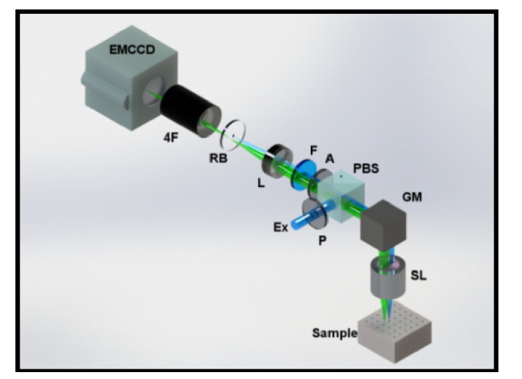
Optical schematic diagram of the 2nd Generation MFMT system. The de-scanned excitation (Ex) light and 2D detector array (EMCCD) compose the system backbone. Polarizing beam splitter (PBS) and cross-polarizers (P, A) minimize specular reflection from the sample surface along with the fluorescence filter (F). Scan lens (SL) and a tube lens form a conjugate image plane and 4F relay system forms the final image on the EMCCD. In higher binning configurations, the spatial integration of the photons deteriorates the dynamic range so a reflection block (RB) is introduced into the system. One set of images is completed after completing a raster scan.
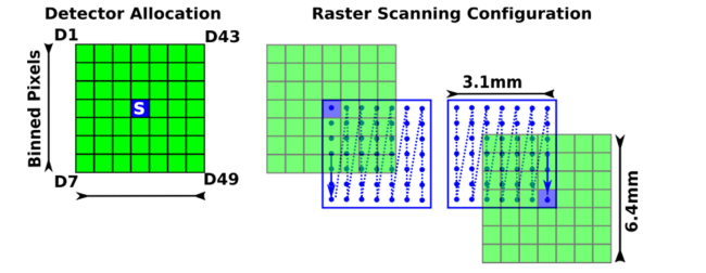
The relative positions of source and detector locations as imaged on the specimen by our system are shown in Fig. 2, where the blue square represents the source, green squares represent the detectors, and the blue dots represent the scanning positions on the surface of the specimen. This depiction renders an acquisition mode with 2 × 2 binning, leading to a total of 256 × 256 detectors covering a FOV of ~6.4 × 6.4 mm2. Of those detectors, we selected an appropriate source-detector separation (~0.6 mm) for 49 detectors in a square grid formation (central detector is occluded due to RB). The source and detectors are moving together as indicated by the blue arrow and the source is always in the center of the detector array. The software-controlled raster scanning step size and dwell times are typically set to 100μm and 20ms, respectively. The typical FOV for illumination is 3.1 × 3.1 mm2, leading to a total of 961 scanning points [12].
Fig. 2.
Schematic diagram of locations of source (blue square), detectors binned from EMCCD camera (green squares), scanning positions on the specimen (blue dots), and scanning path (blue arrows) of the 2nd generation MFMT system.
2.2 The forward model
An accurate forward model, describing the photon propagation inside biological tissues and matching experimental configurations with collected measurements, is critical for every inverse-based tomography technique [13]. Since MFMT operates in the mesoscopic regime, the Monte Carlo (MC) method is used to build the forward model. More specifically, we employ a graphics processing unit (GPU)-based MC code to calculate continuous-wave Green’s functions at excitation and emission wavelengths and [14], and compute the weight function W with an adjoint formulation for efficiency [15]:
| (1) |
where is the lifetime of the fluorophore, and , , and are locations for source, detector and any point inside the specimen being studied. Since the relative location of the source and detectors is fixed, we take one source position and simulate all the source-detector pairs. Then, to match the raster scanning configuration of the system, we populate the sensitivity matrix over the scanned points of the target geometry.
The 3-D distribution of the fluorophore’s effective quantum yield can be revealed by solving the integral equation below:
| (2) |
where is the fluorescence intensity measured at detector location and time when source is used for excitation. As at this time our experimental system is limited to the continuous wave (CW) data type for MFMT applications, both Eqs. (1) and (2) are integrated over time. In order to numerically solve Eq. (2), we discretize the Region of Interest (ROI) into voxels or tetrahedrons based on targeted resolution and transform (2) into a linear equation system:
| (3) |
where ϵ is the sensitivity matrix, or Jacobian, representing effective quantum yield in each discretized element and ϵ is the measurement vector, which represents the detector readings for all source positions. In this paper, the voxel-based MCX is adopted for generating all the Green’s functions in the Jacobian calculation [16].
2.3 The inverse problem
MFMT is by nature an ill-posed inverse problem due to the diffuse nature of the light collected and the limited projection angle offered by the reflectance geometry. As a result, regularization methods have to be applied to obtain robust and accurate reconstructions. Herein, instead of the commonly used -norm regularization, also known as Tikhonov regularization, we take advantage of the sparsity of fluorophore distribution and adopt an -norm regularization scheme [17, 18], expressed as the following optimization problem:
| (4) |
where is the norm of the reconstructed fluorophore distribution vector, and is the regularization parameter, usually determined through an -curve. The minimization problem is convex and then solved with an iterative shrinkage-thresholding algorithm [19].
3. Data reduction strategies for MFMT
The use of an EMCCD camera enables collecting a massive amount of spatial measurements within a short period, leading to potentially increased quality of MFMT reconstruction. However, such a data set is characterized by high redundancy due to scattering and potentially high variance in SNR among different detectors due to large dynamical range. Hence, it is expected that data reduction methodologies aiming at extracting the most informative and robust measurements would lead to better reconstruction accuracy. Herein, we investigate a post-processing methodology that first selects a sub-set of data based on quality measurement criteria and second, uses PCA for further data reduction.
3.1 Data reduction based on SNR/CNR
First, we define the Signal-to-Noise Ratio (SNR) and Contrast-to-Noise Ratio (CNR) of one specific detector as:
| (5) |
| (6) |
where is the fluorescence signal collected at the emission wavelength from all source positions, and is the background signal, defined as the mean of within the Region of Interest (ROI). is also the fluorescence signal collected at the same wavelength and source positions, but with the sample replaced by a beam dump. and stand for the mean and the standard deviation of the signal, separately. In other words, is defined as the true signal intensity and indicates the noise due to sample readout excluding the system noise; thus SNR is the ratio of the signal mean by the standard deviation of noise, and CNR is the ratio of the signal range to the standard deviation of noise.
Detectors with either low average SNR or low CNR readings are then discarded, and the corresponding rows in the sensitivity matrix are truncated as well. As a result, the overall quality of the measurements is improved and the size of the inverse problem is also reduced.
3.2 Data reduction based on PCA
After removing measurements deemed poor based on and criteria, we address the data redundancy by using Principal Component Analysis (PCA). PCA has been proved to be an effective method of extracting useful information from large data sets in numerous fields, including Fluorescence Molecular Tomography (FMT) [20–22]. To filter out correlated measurements and further reduce the size of the inverse problem, we apply PCA on MFMT data sets following the methodology described below.
First, the covariance matrix of the original sensitivity matrix is calculated as , followed by an eigenvalue decomposition of the covariance matrix:
| (7) |
where P is the matrix of columns of eigenvectors of C and Λ is a diagonal matrix with the elements of eigenvalues of the covariance matrix. The inverse problem we want to solve changes from (3) to the following form:
| (8) |
If we only retain the first principal components and leave out the less significant ones, the dimensions of the sensitivity matrix as well as the measurement vector are reduced and (8) becomes:
| (9) |
where is a sub-matrix of , containing only the first rows of , i.e., the largest eigenvectors (out of in total) of the covariance matrix. The number of preserved principal components is typically determined by the cumulative percent of total variance (), defined as:
| (10) |
When the value of reaches a specific threshold, such as 95% or 99%, we set the value of to , and the new sensitivity matrix , while the new measurement vector Through principal component analysis, the redundant information can be effectively suppressed and the reconstruction process is significantly accelerated.
3.3 Evaluation of MFMT reconstruction results
Four metrics are adopted to quantify the difference between reconstruction results and the ground truth, namely, normalized sum squared difference (), normalized sum absolute difference (), normalized disparity (), and correlation () [23].
Suppose we have voxels in a cubic phantom, where are the number of voxels along the and axes. , are the normalized numerical model and reconstructed results with values between 0 and 1 after all negative reconstructed values are set to 0 where and are defined as:
| (11) |
| (12) |
Having a similar trend in and indicate the absence of outlier voxel values in the reconstruction. The values of correlation () and normalized disparity () are calculated as:
| (13) |
| (14) |
where , are binaries (0 or 1) of , through thresholding and represents the exclusive or (XOR) operation. It’s easy to notice that the values of all four metrics lie between 0 and 1, and larger values always indicate a higher similarity with the ground truth, i.e., reconstruction with higher quality.
4. In silico and experimental validation
4.1 Simulation settings
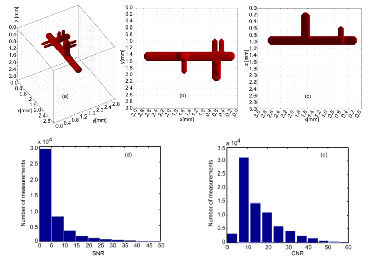
A numerical phantom was designed to evaluate the performance of the proposed algorithm and displayed in Fig. 3. The imaging domain had a surface area of 3.1 × 3.1mm2 with a depth of 3mm. This domain was discretized into 31 × 31 × 30 cubic voxels, leading to 100μm3 element of volumes. A vascular tree with main trunk and three groups of offshoots was simulated deep within the phantom (z = 1mm). The diameter of the trunk was set to 400μm whereas it was set to 200μm for the offshoots. The separation between two adjacent off shoots was set at 100μm (discretization level). The fluorophore concentration was assumed to be uniform in the vessel with effective quantum yield equal to 1 (for simplicity). The whole domain was assumed to be homogeneous at the excitation wavelength with absorption coefficient μa = 0.002mm−1, scattering coefficient μs' = 1 mm−1, index of refraction n = 1.34, and anisotropy factor g = 0.81. These optical properties are derived from the collagen scaffold typically employed in our bio-printing application at collagen density of 6-9 mg/ml [5,9].
Fig. 3.
The numerical phantom designed to mimic vascular structure with a main bio-printed vascular channel and sprouting capillaries. The main trunk has a diameter of 400μm and the off-shoot branches are 200μm in diameter and separated with one voxel spacing to test the resolution of the proposed method. (a), (b) and (c) are the full view, xy view, and xz view of the phantom, respectively. (d) and (e) show the SNR and CNR levels of the synthetic measurements.
To generate in silico measurements, we replicated the imaging system configuration as used in real experiments: 961 illumination scanning positions and 48 detectors at each source location. This configuration yields a Jacobian with size of 46,128 by 28,830 elements. For computational ease and since the study is comparative by nature, we generated the measurements by multiplying the sensitivity matrix with the bio-printed vasculature model. Though, this approach leads to measurements with excellent SNR whereas experimental data can yield SNRs as low as 2. Hence, we added a spatially variant Gaussian noise that replicates the SNR levels seen experimentally. In simulation, we generated the noisy measurements by adding the pure measurements with the noise produced from a normal distribution with mean 0 and standard deviation determined by SNR. For the synthetic measurements we also investigate the dynamic range of the specific noise level in terms of SNR and CNR (see Fig. 3 (d) and (e)). Note that we are not able to calculate the SNR value of one source-detector pair for real experimental data, so the SNR value of one detector (961 source positions) is calculated as in Eq. (5) and used for filtering instead. Then reconstructions are performed as described above. For each of the following simulations or experiment cases, the optimal regularization parameter for the -norm reconstruction algorithm is chosen from an -curve analysis as well as visual inspection.
All computations carried to generate the Jacobians and synthetic measurements were performed under less than 5 minutes in a desktop computer (CPU Intel® Core i7-3820 Quad-Core 3.60 GHz 10MB Intel Smart Cache LGA2011, GPU Quadro K620). Although the reconstructions were performed on the same computer mentioned above, computational time is highly depends on the scale of measurements, Jacobians, and the algorithms adopted as exemplified in the following sections.
4.2 In silico results under different data reduction methods
4.2.1 Data reduction via random sampling
To objectively assess the efficiency of the proposed data reduction, we first established the performance of data reduction via random depopulation of the sensitivity matrix. To ensure that the image-derived metrics are not affected by the stochastic nature of the random approach, ten trials were performed for each set level of data reduction reported. A summary of the evaluation metrics as well as computational times versus level of data reduction is provided in Fig. 4(a). Figures 4(b) and 4(c) also provide a visual validation for the effect of random sampling for two specific levels of data reduction.
Fig. 4.
Reconstruction results and evaluation metrics under random sampling. (a) plots the average metrics of reconstructions with different numbers of remaining measurements. (b) and (c) show two visual reconstruction results with 5,000 and 30,000 measurements left, respectively.
Overall, although random sampling reduces the computation time, there are no obvious improvements on evaluation metrics when a certain data reduction level is implemented. Especially, as the number of measurements used in reconstruction is reduced, the offshoots cannot be resolved and the integrity of the main trunk is compromised (Fig. 4. (b)).
4.2.2 Data reduction based on SNR
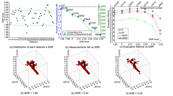
MFMT is an ill-conditioned inverse problem and hence, the quality of the reconstructions is very sensitive to noise. Such sensitivity is typically observed as large artefacts on the surface and/or degradation of the resolution, leading to reconstructions with extremely poor fidelity. Hence, beyond implementing regularization techniques, one can implement a pre-processing data selection methodology that aims at discarding any detector readings with low SNR before proceeding to the reconstruction. An example of SNR distribution of each of the 48 detectors over 961 sources is provided in Fig. 5(a). From this distribution, a low SNR threshold can be defined and implemented such that any detector reading below this threshold is not considered in the inverse problem. For different values of this threshold, the number of measurements left and computation times are shown in Fig. 5(b) while the evaluation metrics of corresponding reconstruction results are shown in Fig. 5(c). The reconstructions associated with three specific threshold values are provided in Figs. 5(d-f). From these simulation results, we can see that removing detectors with lower SNR improves the quality of reconstruction and outperforms the random data reduction approach. However, if the threshold value is set too high, the reconstruction quality is compromised, as visually illustrated in Figs. 5(d-f). Hence, an optimal SNR threshold has to be determined based on the SNR level of the acquired data set as well as the amount of data points available.
Fig. 5.
Reconstruction results and evaluation metrics under SNR-based data reduction strategy. (a) gives the distribution of the 48 detectors’ SNR level in a case scenario. (b) plots the computation time and measurements left corresponding to different threshold of SNR. (c) plots the 4 metrics versus different threshold of SNR. (d)-(f) show 3 visual reconstructions with retained measurements after filtering by the specific SNR threshold of 1.99, 2.02, and 2.05, respectively.
4.2.3 Data reduction based on CNR
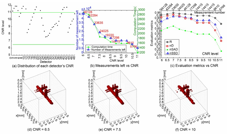
It is imperative not to cull the data too drastically based on SNR. It remains that some detector readings, while having good SNR, contribute little to revealing the fluorophore distribution due to the lack of image contrast. Therefore, they can also be considered as redundant data and could be removed. Similar to the SNR-based case, we calculated the CNR values of 48 detectors from all 961 source positions, and plot the CNR distribution, numbers of measurements left and time costs in Figs. 6(a-b). The results under different CNR levels, as shown in Figs. 6(c-f), also follow the same trend as for the SNR-based case: the reconstructions improve as detectors with low CNR are discarded, but then worsen with increasing the CNR cutoff value.
Fig. 6.
Reconstruction results and evaluation metrics under CNR-based data reduction strategy. (a) gives the distribution of the 48 detectors’ CNR level in a case scenario. (b) plots the computation time and measurements left corresponding to different thresholds of CNR. (c) plots the 4 metrics versus different thresholds of CNR. (d)-(f) show 3 visual reconstructions with retained measurements after filtering by the specific CNR threshold of 6.5, 7.5, and 10, respectively.
4.2.4 Data reduction via PCA
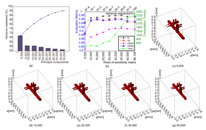
To investigate the performance of PCA-derived data reduction on MFMT reconstructions, we retained the largest principal components k, from 5,000 to 40,000 out of 46,128. The cumulative percent of total variance is plotted in Fig. 7(a), while the computation times and values of evaluation metrics are shown in Fig. 7(b). As shown, the reconstruction quality improves significantly when k rises from 5,000 to 10,000, but then remains relatively stable when k varies from 10,000 to 35,000, and then degrades as k continues to increase to 40,000 until all components are used. These results are in accordance with the expectation that the majority of the information in the Jacobian can be represented with a much smaller dimension – in our case >80% of CPV explained with <33% of the largest components. Also because the measurements are noisy and highly redundant, introducing more principal components is not expected to bring additional useful information, but only amplify the noise effect instead, as visually validated in Figs. 7(c-g).
Fig. 7.
Reconstruction results and evaluation metrics under PCA-based data reduction strategy in a simulation. (a) gives the relationship between variance explained and different principal components in a simulation. (b) plots the computation time and 4 metrics versus measurements left corresponding to different thresholds of CPV. (c)-(g) show 5 visual reconstructions with retained measurements after filtering by the specific CPV threshold of 67.4, 81.2, 90.7, 95.8, and 97.5, respectively.
To further demonstrate the benefit of PCA, we provide a detailed comparison in Table 1 between when no PCA is applied and when only the 35,000 largest components are retained. Despite the decrease in Jacobian size and time cost when applying PCA, all four evaluation metrics are higher compared to the original result. PCA is thus proven to be effective in both accelerating the inverse problem and improving the quality of reconstruction.
Table 1. Quantification results of the two methods in the numerical simulation (CPV = 95.8%).
| Methods | Sensitivity matrix size | Reconstruction time(s) | R | nD | nSAD | nSSD |
|---|---|---|---|---|---|---|
| Without PCA | 46,128 × 28,830 | 2,786 | 0.952 | 0.941 | 0.912 | 0.928 |
| With PCA | 35,000 × 28,830 | 1,937 | 0.981 | 0.963 | 0.918 | 0.964 |
4.3 Summary of quantification results for data reduction methods on simulation data
Here we give a table to shortly summarize the quantification results for the above mentioned simulations. As shown in the Table 2, although reconstruction time is basically affected by the size of sensitivity matrix, it highly depends on the property of sensitivity matrix, such as sparse, correlation of components. In addition, the preset thresholds of SNR/CNR or CPV have a huge impact on the size of sensitivity matrix and reconstruction quality, as shown in Fig. 4 to Fig. 7. Note that we set different thresholds of SNR/CNR or CPV in order to achieve high quality reconstruction in different cases.
Table 2. Quantification results of the methods adopted for synthetic measurements.
| Methods | Sensitivity matrix size | Reconstruction time (s) | Regularization parameter |
|---|---|---|---|
| Full data | 46,128 × 28,830 | 2,942 | 0.016 |
| After SNR filter (threshold = 2.02) | 27,869 × 28,830 | 2,100 | 0.753 |
| After CNR filter (threshold = 7.5) | 24,025 × 28,830 | 1,896 | 0.005 |
| After PCA reduction (CPV = 95.8%) | 35,000 × 28,830 | 1,937 | 0.259 |
| After SNR, CNR filter (threshold of SNR = 2.0/CNR = 6.5) | 37,479 × 28,830 | 2,178 | 0.896 |
| After SNR, CNR filter & PCA (threshold of SNR = 2.0/CNR = 6.5/CPV = 95%) | 28,123 × 28,830 | 1,484 | 0.001 |
4.4 Performance of data reduction on experimental data
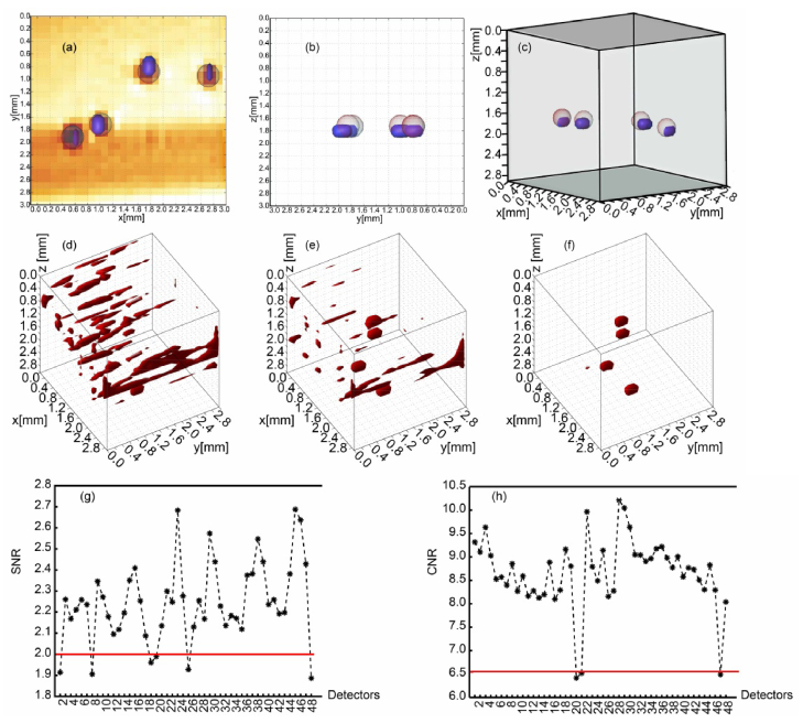
Last we applied the proposed two-step data reduction algorithm on an experimental data set, acquired from a collagen sample with optical properties μa = 0.002 mm−1, μs' = 1 mm−1, n = 1.34, and g = 0.81. The sample size was 3.1 × 3.1 × 3.0mm3, with four polystyrene fluorophore beads (GFP 488/509, Cospheric) placed 1.7~1.8 beneath the sample surface following standard protocols. The voxel size of 100 × 100 × 100μm3 is also employed for the experimental phantom. Transversal micro-MRI slices taken across the x-y and y-z planes are shown in Figs. 8(a-b). As in the simulation configuration, the source scans over 31 × 31 positions and measurements of 48 detectors are collected at each source position in less than 20ms.
Fig. 8.
Phantom reconstruction under the proposed redundant data reduction method. (a) segmented micro-MRI slice and reconstruction across x-y plane. (b) segmented micro-MRI slice and reconstuction across y-z plane. (c) 3D overlaid image of micro-MRI and optimal reconstruction. (d) reconstruction result using full data. (e)reconstruction result based on the remaining data after noise suppression. (f) reconstruction results using the retained data after both noise suppression and PCA processing. (g) and (h) are the distributions of SNR and CNR of 48 detectors.
The reconstruction with the original sensitivity matrix and measurements was initially performed. Then, for the first step of data reduction, we discarded detector readings with low SNR and low CNR sequentially and carried out a second reconstruction based on the simulation results. According to the simulation results the thresholds of SNR and CNR were optimally set to 2 and 6.5, leading to the removal of 6 detectors (5,766 measurements) and 3 detectors (2,883 measurements), respectively (see Fig. 8 (g-h)). Lastly, for the second step of data reduction, we applied PCA to the trimmed Jacobian from the last step. The CPV value was set to 95%, corresponding to 28,123 principal components, and a third reconstruction with the data-reduced Jacobian and measurement vector was conducted. All three inverse problems were solved with our L1 reconstruction algorithm as described in section 2.3 and the optimal regularization parameters were determined through L-curves.
The 3D reconstruction results for the above three cases are shown in Table 3 and Figs. 8(d-f). Compared to the original case, the artifacts are remarkably suppressed after data points with low SNR/CNR measurements are removed. However the accurate locations and shapes of four beads are still not satisfactory compared to micro-MRI. After applying the PCA data reduction approach, the artifacts are completely eliminated while the locations and depths of beads match perfectly with those in the micro-MRI images, shown in Figs. 8(a-c). Hence, these results demonstrate that the sequential combination of SNR/CNR with PCA data reduction approaches leads to faster as well as improved reconstruction performances.
Table 3. Quantification results of the methods for experimental data (threshold of SNR = 2.0/CNR = 6.5/CPV = 95%).
| Methods | Sensitivity matrix size | Reconstruction time (s) | Regularization parameter |
|---|---|---|---|
| Full data | 46,128 × 28,830 | 2,942 | 7.352 |
| After SNR filter | 40,362 × 28,830 | 2,786 | 6.320 |
| After CNR filter | 43,245 × 28,830 | 2,816 | 1.589 |
| After PCA reduction | 35,000 × 28,830 | 1,958 | 0.002 |
| After SNR, CNR filter | 37,479 × 28,830 | 2,210 | 1.402 |
| After SNR, CNR filter & PCA | 28,123 × 28,830 | 1,556 | 0.735 |
5. Conclusions
In conclusion, we have presented a comprehensive data reduction method on an MFMT data set, where measurements with low SNR/CNR are first removed and PCA is then applied for dimension reduction. With the proposed method, the noise and redundancy in MFMT raw data are minimized while the most useful information revealing fluorophore distribution is retained. We have tested the performance of the data reduction algorithm on data sets from numerical simulations as well as real experiments. In both cases, the performances of the reconstruction were significantly improved in terms of spatial accuracy as well as computational efficiency. In the case of the experimental study, locations and shape of the imaged objects were retrieved with high fidelity (resolution <200 µm) even though they were deeply embedded (z = 1.8 mm) in a highly scattering medium (μs' = 1 mm−1). We expect that this methodology will support our efforts in monitoring longitudinally bio-printed tissues [12] and in vivo tumor xenografts [8]. Additionally, beyond MFMT and/or CW data sets, we will investigate the utility of this data processing methodology for applications relying on temporal and/or spectral data sets such as those acquired in our novel hyperspectral time-resolved imager [24, 25].
Funding
National Institutes of Health (NIH) (R01-EB019443 and R01 BRG-CA207725); National Science Foundation (NSF) (Career Award CBET 1149407); Natural Science Foundation of Shandong Province (ZR2014FL031); National Natural Science Foundation of China (61472227); Science and Technology Project of Yantai (2015ZH059).
References and links
- 1.Hillman E. M., Boas D. A., Dale A. M., Dunn A. K., “Laminar optical tomography: demonstration of millimeter-scale depth-resolved imaging in turbid media,” Opt. Lett. 29(14), 1650–1652 (2004). 10.1364/OL.29.001650 [DOI] [PubMed] [Google Scholar]
- 2.Yuan S., Li Q., Jiang J., Cable A., Chen Y., “Three-dimensional coregistered optical coherence tomography and line-scanning fluorescence laminar optical tomography,” Opt. Lett. 34(11), 1615–1617 (2009). 10.1364/OL.34.001615 [DOI] [PubMed] [Google Scholar]
- 3.Ozturk M. S., Chen C.-W., Ji R., Zhao L., Nguyen B.-N. B., Fisher J. P., Chen Y., Intes X., “Mesoscopic Fluorescence Molecular Tomography for Evaluating Engineered Tissues,” Ann. Biomed. Eng. 44(3), 667–679 (2016). 10.1007/s10439-015-1511-4 [DOI] [PMC free article] [PubMed] [Google Scholar]
- 4.Dunn A., Boas D., “Transport-based image reconstruction in turbid media with small source-detector separations,” Opt. Lett. 25(24), 1777–1779 (2000). 10.1364/OL.25.001777 [DOI] [PubMed] [Google Scholar]
- 5.Zhao L., Lee V. K., Yoo S.-S., Dai G., Intes X., “The integration of 3-D cell printing and mesoscopic fluorescence molecular tomography of vascular constructs within thick hydrogel scaffolds,” Biomaterials 33(21), 5325–5332 (2012). 10.1016/j.biomaterials.2012.04.004 [DOI] [PMC free article] [PubMed] [Google Scholar]
- 6.Björn S., Englmeier K. H., Ntziachristos V., Schulz R., “Reconstruction of fluorescence distribution hidden in biological tissue using mesoscopic epifluorescence tomography,” J. Biomed. Opt. 16(4), 046005 (2011). 10.1117/1.3560631 [DOI] [PubMed] [Google Scholar]
- 7.Tang Q., Tsytsarev V., Frank A., Wu Y., Chen C. W., Erzurumlu R. S., Chen Y., “In Vivo Mesoscopic Voltage-Sensitive Dye Imaging of Brain Activation,” Sci. Rep. 6(1), 25269 (2016). 10.1038/srep25269 [DOI] [PMC free article] [PubMed] [Google Scholar]
- 8.Ozturk M. S., Rohrbach D., Sunar U., Intes X., “Mesoscopic fluorescence tomography of a photosensitizer (HPPH) 3D biodistribution in skin cancer,” Acad. Radiol. 21(2), 271–280 (2014). 10.1016/j.acra.2013.11.009 [DOI] [PubMed] [Google Scholar]
- 9.Ozturk M. S., Lee V. K., Zhao L., Dai G., Intes X., “Mesoscopic fluorescence molecular tomography of reporter genes in bioprinted thick tissue,” J. Biomed. Opt. 18(10), 100501 (2013). 10.1117/1.JBO.18.10.100501 [DOI] [PMC free article] [PubMed] [Google Scholar]
- 10.Yang F., Ozturk M. S., Zhao L., Cong W., Wang G., Intes X., “High-Resolution Mesoscopic Fluorescence Molecular Tomography Based on Compressive Sensing,” IEEE Trans. Biomed. Eng. 62(1), 248–255 (2015). 10.1109/TBME.2014.2347284 [DOI] [PMC free article] [PubMed] [Google Scholar]
- 11.Ouakli N., Guevara E., Dubeau S., Beaumont E., Lesage F., “Laminar optical tomography of the hemodynamic response in the lumbar spinal cord of rats,” Opt. Express 18(10), 10068–10077 (2010). 10.1364/OE.18.010068 [DOI] [PubMed] [Google Scholar]
- 12.Ozturk M. S., Intes X., Lee V. K., “Longitudinal Volumetric Assessment of Glioblastoma Brain Tumor in 3D Bio-Printed Environment by Mesoscopic Fluorescence Molecular Tomography,” in Optics and the Brain, (Optical Society of America, 2016), JM3A. 46. [Google Scholar]
- 13.Arridge S. R., Schotland J. C., “Optical tomography: forward and inverse problems,” Inverse Probl. 25(12), 123010 (2009). 10.1088/0266-5611/25/12/123010 [DOI] [Google Scholar]
- 14.Fang Q., Boas D. A., “Monte Carlo Simulation of Photon Migration in 3D Turbid Media Accelerated by Graphics Processing Units,” Opt. Express 17(22), 20178–20190 (2009). 10.1364/OE.17.020178 [DOI] [PMC free article] [PubMed] [Google Scholar]
- 15.Chen J., Intes X., “Comparison of Monte Carlo methods for fluorescence molecular tomography-computational efficiency,” Med. Phys. 38(10), 5788–5798 (2011). 10.1118/1.3641827 [DOI] [PMC free article] [PubMed] [Google Scholar]
- 16.Fang Q., “Monte Carlo eXtreme (MCX),” http://mcx.space/.
- 17.Zhao L., Yang H., Cong W., Wang G., Intes X., “Lp regularization for early gate fluorescence molecular tomography,” Opt. Lett. 39(14), 4156–4159 (2014). 10.1364/OL.39.004156 [DOI] [PMC free article] [PubMed] [Google Scholar]
- 18.Yao R., Pian Q., Intes X., “Wide-field fluorescence molecular tomography with compressive sensing based preconditioning,” Biomed. Opt. Express 6(12), 4887–4898 (2015). 10.1364/BOE.6.004887 [DOI] [PMC free article] [PubMed] [Google Scholar]
- 19.Beck A., Teboulle M., “A Fast Iterative Shrinkage-Thresholding Algorithm for Linear Inverse Problems,” SIAM J. Imaging Sci. 2(1), 183–202 (2009). 10.1137/080716542 [DOI] [Google Scholar]
- 20.Mohajerani P., Ntziachristos V., “Compression of Born ratio for fluorescence molecular tomography/x-ray computed tomography hybrid imaging: methodology and in vivo validation,” Opt. Lett. 38(13), 2324–2326 (2013). 10.1364/OL.38.002324 [DOI] [PubMed] [Google Scholar]
- 21.Cao X., Wang X., Zhang B., Liu F., Luo J., Bai J., “Accelerated image reconstruction in fluorescence molecular tomography using dimension reduction,” Biomed. Opt. Express 4(1), 1–14 (2013). 10.1364/BOE.4.000001 [DOI] [PMC free article] [PubMed] [Google Scholar]
- 22.Zhang J., Shi J., Zuo S., Liu F., Bai J., Luo J., “Fast reconstruction in fluorescence molecular tomography using data compression of intra- and inter-projections,” Chin. Opt. Lett. 13(7), 071002 (2015). 10.3788/COL201513.071002 [DOI] [Google Scholar]
- 23.Silva J. S., Cancela J., Teixeira L., “Fast volumetric registration method for tumor follow-up in pulmonary CT exams,” J. Appl. Clin. Med. Phys. 12(2), 3450 (2011). 10.1120/jacmp.v12i2.3450 [DOI] [PMC free article] [PubMed] [Google Scholar]
- 24.Pian Q., Yao R., Sinsuebphon N., Intes X., “Compressive Hyperspectral Time-resolved Wide-Field Fluorescence Lifetime Imaging,” Nat. Photonics. 11411–417 (2017). [DOI] [PMC free article] [PubMed] [Google Scholar]
- 25.Pian Q., Yao R., Zhao L., Intes X., “Hyperspectral time-resolved wide-field fluorescence molecular tomography based on structured light and single-pixel detection,” Opt. Lett. 40(3), 431–434 (2015). 10.1364/OL.40.000431 [DOI] [PMC free article] [PubMed] [Google Scholar]


