A parametric model to estimate the proportion from true null using a distribution for p-values

Abstract

Microarray studies generate a large number of p-values from many gene expression comparisons. The estimate of the proportion of the p-values sampled from the null hypothesis draws broad interest. The two-component mixture model is often used to estimate this proportion. If the data are generated under the null hypothesis, the p-values follow the uniform distribution. What is the distribution of p-values when data are sampled from the alternative hypothesis? The distribution is derived for the chi-squared test. Then this distribution is used to estimate the proportion of p-values sampled from the null hypothesis in a parametric framework. Simulation studies are conducted to evaluate its performance in comparison with five recent methods. Even in scenarios with clusters of correlated p-values and a multicomponent mixture or a continuous mixture in the alternative, the new method performs robustly. The methods are demonstrated through an analysis of a real microarray dataset.

1. Introduction

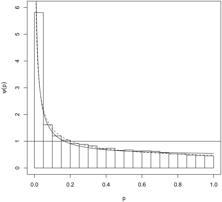
Microarray studies generate a large number of p-values from comparisons of gene expression data. The p-values are usually generated using statistical tests. To give an example, Figure 10 shows the histogram of a typical set of such p-values. In the experiment, the expression of 12, 488 genes was measured on B lymphocytes. The B lymphocytes were harvested from two types of mice (factor 1); and the cells were either treated with an anti-IgM antibody or not treated (factor 2). The p-values were obtained using the Kruskal-Wallis test (Kruskal and Wallis, 1952) for a group effect on the expression data. The group was defined by the two experimental factors. The test is asymptotically chi-squared with 3 degrees of freedom (df). The study that generated these p-values is described in detail in Section 5.

Figure 10.

Two fitted parametric models to the MALT dataset analyzed in Pounds and Morris (2003). The solid line is the fitted mixture model (5) with (3) as the non-null component ψ for the chi-squared test. The dashed line represents the fitted beta uniform mixture model of Pounds and Morris (2003).

Based on the p-values, investigators want to infer which of the tested genes are impacted by the experiment factors using multiple testing procedures. In these procedures, such as those of Benjamini and Hochberg (2000), Efron, Tibshirani et al. (2001), Efron and Tibshirani (2002), among others, the proportion of the p-values which are from data under the null hypothesis plays an important role. We denote this proportion as π₀. There has been great interest in how to estimate this proportion. Broberg (2005) reviews six methods and proposes two new methods to estimate this proportion. More recent developments are by Langaas, Lindqvist, and Ferkingstad, 2005; Cheng, 2006; Nettleton et al., 2006; Meinshausen and Rice, 2006; Tang, Ghosal, and Roy, 2007; Markitsis and Lai, 2010.

If the data are generated under the null hypothesis, then the p-values follow the uniform distribution. There has been little research on parametric distributions for the p-values generated from data under an alternative hypothesis. Nevertheless, the proportion π₀ is often estimated using a two-component mixture model such as many of the methods in the above references. Specifically, let 100π₀–percent (0 < π₀ < 1) of the p-values be sampled from the uniform (0, 1) and the remaining 100(1 – π₀)–percent be sampled from a distribution denoted by ψ(p). This is the distribution of the p-values sampled from data under an alternative. Then the mixed p-values have the marginal distribution with density function

$$f(p)={\pi }_0+(1-{\pi }_0)\psi (p).$$ (1)

There is literature on nonparametric methods to model the mixture of p-values. The mixing parameter π₀ is generally not identifiable due to the simultaneously unknown ψ(p). In order to solve this identifiability problem, the methods of Langaas, Lindqvist, and Ferkingstad (2005), Tang, Ghosal, and Roy (2007) impose restrictions such as monotonically decreasing and ψ(1) = 0 on ψ(p). In Section 2 we show that the ψ(1) = 0 restriction may be a good approximation when the alternative hypothesis is far away from the null, but it is generally not true. Others, such as those summarized in Broberg (2005) and Cheng (2006), estimate an upper-bound of π₀ instead of π₀ itself; and Meinshausen and Rice (2006) estimate a lower-bound of 1 – π₀.

Among the eight methods in Broberg (2005) to estimate π₀, only Pounds and Morris (2003) explicitly assume a parametric beta uniform mixture. Their objective is to extract a uniform component from the mixture density in order to estimate an upper-bound of π₀. Markitsis and Lai (2010) further develop this beta uniform mixture model by censoring p-values less than a cutoff to improve the estimate. All the other seven methods in Broberg (2005) are non-parametric. Other limited parametric methods also mainly focus on beta or beta mixtures (Parker and Rothenberg, 1988; Allison, Gadbury et al., 2002; Xiang, Edwards, and Gadbury, 2006). Diaconis and Ylvisaker (1985) suggest that a distribution on the interval [0, 1] can be modeled as a finite mixture of beta distributions. Parker and Rothenberg (1988) fitted this model to a set of 1, 113 p-values obtained using t-tests in sub-group analyses. Allison, Gadbury et al. (2002) applied a similar idea of beta mixtures to model p-values obtained in microarray studies. Their goodness of fit indicates that the finite mixture of beta distributions provides a reasonable fit to the p-values. However, none of these works provide a theoretical basis as to why the distribution of p-values can be modeled as beta distributions or their mixtures.

In Appendix A, we derive a beta distribution for the p-values. It is derived only for the case that the distribution functions of the test statistic under the null and under the alternative differ by the Lehmann alternative through their survival functions. For some common tests such as the normal test and the t-test, their distribution ψ(p) of the p-values from data under an alternative is not beta.

Lack of understanding about the parametric form of the distribution of p-values from data under the alternative hypothesis tilts current research in estimating π₀ almost entirely toward nonparametric methods (Broberg, 2005; Langaas, Lindqvist, and Ferkingstad, 2005; Cheng, 2006; Nettleton et al., 2006; Meinshausen and Rice, 2006; Tang, Ghosal, and Roy, 2007). The aim of this work is to develop a parametric distribution for p-values sampled under the alternative hypothesis and use this distribution to estimate π₀ for a specific test statistic. Pounds and Morris (2003) generated a sample of p-values using chi-squared tests. We develop the method for the chi-squared test and demonstrate the method on this dataset. The common model-based Wald test is asymptotically chi-squared test. The normal test can be transformed into chi-squared test, and the t-test can be transformed into asymptotic chi-squared test when the degree of freedom is large. Thus, the methods we developed for the chi-squared test could be applied broadly in data analyses. Nevertheless, the method can be readily modified to other reference statistics.

The rest of the manuscript is organized as follows. In Section 2, we derive the distribution (3) for p-values obtained using the chi-squared test. In Section 3, under the two-component mixture model (1), we develop the MLE of π₀ and the non-null component ψ(p) represented by the non-centrality parameter λ of the reference chi-squared distribution. We further present a gamma mixture model for a range of alternatives. Section 4 reports simulation studies for a variety of scenarios to evaluate our method in comparison with five recent methods. We revisit the data example analyzed by Pounds and Morris (2003) in Section 5. We conclude the manuscript by a discussion in Section 6.

2. The distribution of p-values from the chi-squared test

Consider a chi-squared test statistic X with ν df. Let its cumulative distribution function be denoted by F(·) and its density function is f(·) under the null hypothesis. Define x_p as the p–th percentile of the statistic X so F(x_p) = p. The test with significance level p will reject the null hypothesis when X > x_1–p.

If the data are generated under the alternative hypothesis, the test statistic asymptotically follows the non-central chi-squared distribution. Following Kruskal and Wallis (1952), this can be shown for the Kruskal-Wallis test with test statistic

$$H=\frac{N-1}{N}\sum _{i=1}^c\frac{n_i{[{\overline{R}}_i-(N+1)/2]}^2}{(N^2-1)/12},$$ (2)

where group i (i = 1, 2, …, c; c ≥ 3) has n_i subjects and an average rank R̄_i, and $N={\sum }_{i=1}^c{n}_i$ is the total sample size. The above test statistic (2) is essentially a sum of squared standardized deviations of random variables from their mean under the null. Thus asymptotically it follows the central or non-central chi-squared distributions under the null or the alternative hypothesis, respectively. The null centrality parameter depends on the specific alternative. A similar argument can be made for the traditional chi-squared test where the test statistic is defined as a sum of the squared standardized difference between the observed and the expected under the null. This distributional result is also true for some of the common model-based chi-squared tests, such as the score test and the Wald test.

Suppose the statistic has a non-central chi-squared distribution with non-centrality parameter λ > 0 and ν df. Let g(·) denote the corresponding non-central chi-squared probability density function. The distribution for p-values under the alternative can be derived as

$$\psi (p)=g(x_{1-p})/f(x_{1-p}).$$

Details of the derivation are in Appendix A. Specifically for the chi-squared test, the density function can be expressed as

$$\begin{array}{c}\psi (p)=\sum _{j=0}^{\infty }\left\{\frac{{(\lambda /2)}^j}{j!}{e}^{-\lambda /2}\right\}\frac{f(x_{1-p};\nu +2j)}{f(x_{1-p};\nu )}\\ =e^{-\lambda /2}+\sum _{j=1}^{\infty }\left\{\frac{{(\lambda /2)}^j}{j!}{e}^{-\lambda /2}\right\}\frac{x_{1-p}^j}{(\nu +2j-2)(\nu +2j-4)\cdots \nu },\end{array}$$ (3)

where x_1–p is the upper p–th quantile of F.

The intuitive interpretation of this distribution is that the density of the p-values is a weighted sum of the ratios of two central χ² densities with ν + 2j and ν df, respectively, for j = 0, 1, …. The weights are the probabilities of a Poisson distribution with mean λ/2.

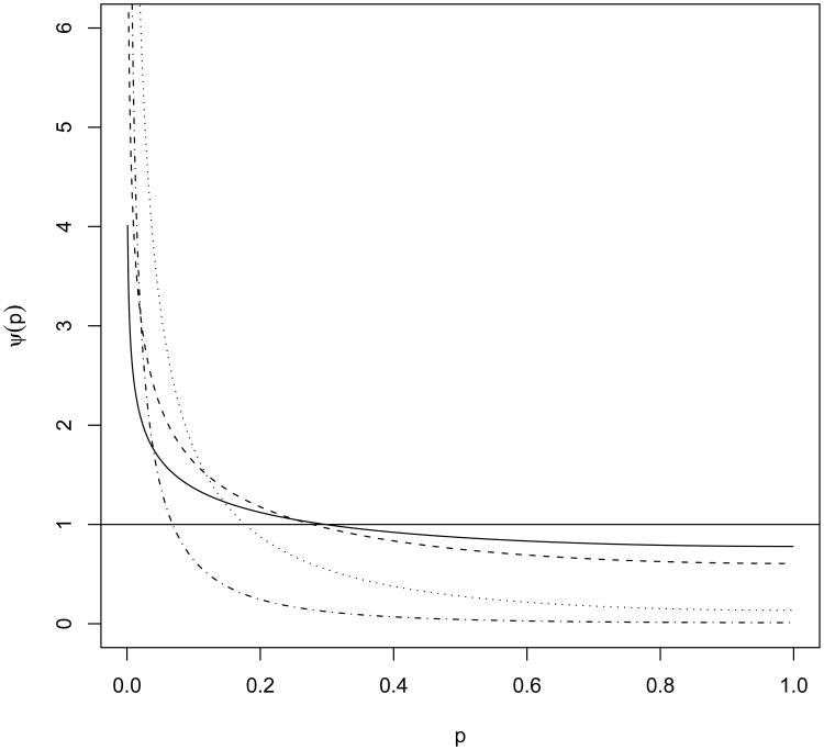
When λ = 0, corresponding to the null hypothesis, distribution (3) reduces to uniform [0, 1]. In Appendix A, we prove that the density (3) is monotonically decreasing on [0, 1]. It reaches its minimum at ψ(1) = e^−λ/2. Density (3) can also be rewritten as a polynomial of the quantile

$$\psi (p)=\sum _{j=0}^{\infty }{w}_j{x}_{1-p}^j,$$

where

$$w_j=\left\{\frac{{(\lambda /2)}^j}{j!}{e}^{-\lambda /2}\right\}\frac{\mathrm{\Gamma }(\nu /2)}{2^j\mathrm{\Gamma }(\nu /2+j)}.$$

When we compute (3), the summands diminish quickly for λ not large since the Poisson probability weight becomes small as j increases. In general, the limit of j needs to be sufficiently large relative to both ν and λ/2 so that the omitted terms are negligible. The numerical evaluation and simulations in Section 4 indicate that a limit of 30 for j is sufficient for a broad range of applications. We set the limit of j to 30 to cut down the simulation time. In a real data analysis setting, there is no reason the users can not choose a larger limit. We have included this as a variable in the R function so that users can have their own choice when they analyze their data. Similar considerations apply when we compute density (4).

Figure 1 displays the density function ψ(p) with ν = 1 for several values of λ. Under alternative hypotheses, Figure 1 shows that ψ(p) has a shift away from the uniform distribution, favoring smaller p-values that are associated with rejecting the null hypothesis. These curves show that ψ(1) = e^−λ/2 is not zero, although ψ(1) may approach zero when λ → ∞. However, large λ indicates that the alternative is far from the null and the case is not very interesting in hypothesis testing. We want to study situations when λ is small.

Figure 1.

Density function (3) of p-values from a 1 df chi-squared test against a 1 df non-central chi-squared alternative hypothesis with non-centrality parameter λ = .5, 1, 4, 9 as solid, dashed, dotted, and dash-dotted lines, respectively.

In reality it is likely that there are many different alternatives when testing multiple hypotheses such as in microarray studies. This can be accounted for by allowing the non-centrality parameter λ to take a range of different values instead of a unique value as in the model (5). Here we introduce a model in which λ follows a continuous distribution to represent various alternatives.

We assume U = λ/2 in (3) follows a Gamma (k, θ) distribution with a density function

$$h(u;k,\theta )=\frac{1}{\mathrm{\Gamma }(k){\theta }^k}{u}^{k-1}{e}^{-u/\theta }.$$

Then the compound distribution of P under the alternatives can be derived as

$$\begin{array}{c}\psi (p;k,\theta )=\sum _{j=0}^{\infty }{\int }_0^{\infty }\left\{\frac{u^j}{j!}{e}^{-u}\right\}h(u;k,\theta )du\frac{f(x_{1-p};\nu +2j)}{f(x_{1-p};\nu )}\\ =\sum _{j=0}^{\infty }\frac{(j+k-1)!}{j!(k-1)!}{(\theta /(1+\theta ))}^j{(1/(1+\theta ))}^k\frac{f(x_{1-p};\nu +2j)}{f(x_{1-p};\nu )}.\end{array}$$ (4)

Note in (4), the weight in front of the ratio of the two central χ² densities is the probability mass function of a negative binomial distribution NB (k, θ/(1 + θ)). In the data example of Section 5, we fit model (5) using (4) for the distribution of P under a range of alternatives.

3. Estimate of π₀

We first assume that the microarray comprises 100π₀–percent samples from the null hypothesis and 100(1 – π₀)–percent from a single alternative represented by λ. Then the distribution of the mixed p-values has marginal density

$$f(p)={\pi }_0+(1-{\pi }_0)\psi (p|\lambda ).$$ (5)

The density ψ(p | λ) of p under an alternative hypothesis determined by λ > 0 in chi-squared test is derived as (3). The combination of (3) and (5) solves the identifiability problem that has long been encountered in many of the nonparametric estimates of π₀. Maximum likelihood methods can be used to estimate the two parameters π₀ and λ.

$${({\widehat{\pi }}_0,\widehat{\lambda })}^{\prime }=arg\underset{{({\pi }_0,\lambda )}^{\prime }}{max}\sum _{i}log\{{\pi }_0+(1-{\pi }_0)\psi (p_i|\lambda )\}.$$ (6)

For this specific setting, we are unable to obtain closed-form expressions for the MLE's of π₀ and λ, so we have developed R programs to evaluate the log likelihood numerically to obtain the MLE's and their standard errors. The negative of log likelihood (6) is minimized using the optimization routine nlm in R. This routine uses a Newton-type algorithm and it also provides estimates of the Hessian matrix that was used to estimate standard errors reported in Table 1 for the example in Section 5. In the case we use model (4) to account for a range of alternatives, model (5) can be fit similarly to obtain (π̂₀, k̂, θ̂)′ with (4) as the non-null component if the mixture model is identifiable. We will discuss the identifiability issue of model (4) in Section 4.4. We next conduct simulation studies to evaluate the distribution mixture-based method in comparison with five recent methods. Then we demonstrate the methods on a real dataset analyzed by Pounds and Morris (2003).

Table 1.

Six estimates of π₀ for the MALT dataset.

Method	π̂0	95% CI	Method	π̂0	95% CI
Mixture	0.5358	(0.5184, 0.5532)	Storey	0.4525	(0.4249, 0.4813)†
BUM	0.4764	N/A‡	CBUM	0.5017	N/A‡
Meinshausen	0.5549	N/A‡	Nettleton	0.4516	(0.4020, 0.5016)†

^†The CI was obtained by bootstrapping with 1,000 replicates.

^‡The CI was not calculated since the estimate itself is an upper-bound of π₀.

4. Simulation studies

4.1. Methods included for comparison and simulation set-up

In simulation studies, we evaluated the performance of our estimate in comparison with five recent methods. Among these methods, the beta uniform mixture (BUM) model of Pounds and Morris (2003) and a modification of BUM by Markitsis and Lai (2010) are parametric models. The BUM model is the mixture of a uniform and a beta distribution. The mixture's probability density function is

$$f_{\beta }(p|\omega ,a)=\omega +(1-\omega )a{p}^{a-1}$$ (7)

for parameters 0 < ω < 1 and a > 0. Pounds and Morris (2003) set the second parameter in the beta distribution equal to one in order for f_β to be monotonically decreasing in 0 < p < 1. They concluded that it was impossible to estimate the actual π₀. However, their model provides an estimate of the upper bound of π₀ as f_β(1 | ω̂, â) = ω̂ + (1 – ω̂) â. This upper bound was reported in the simulations. Markitsis and Lai (2010) propose a censored beta uniform mixture model (CBUM) by censoring p-values less than a cutoff point to improve the BUM estimate. This CBUM estimate of π₀ was also included in the simulations.

A large number of non-parametric estimates of π₀ are in the literature. We included some of the recent developments in the simulations: the threshold method of Storey and Tibshirani (2003), the histogram-based method (Nettleton et al. 2006), and a method to establish the lower confidence bound for 1 – π₀ based on the empirical distribution of the p-values (Meinshausen and Rice, 2006).

We implemented our estimate in R. For the BUM and Nettleton methods, we downloaded the R programs from the author's website. The CBUM, Storey, and Meinshausen methods are in R packages pi0, qvalue, and howmany, respectively.

The simulations were set up to test the hypotheses H₀ : λ = 0 versus H_a : λ > 0. The test statistic was sampled 100π₀–percent from the central chi-squared distribution with ν = 10 df and 100(1 – π₀)–percent from the non-central chi-squared distribution with ν = 10 df and the non-centrality parameter λ being 4, 9, or 16. The simulated range for π₀ was between 0.05 and 0.95 at increase of 0.05 for the independent case and at increase of 0.1 for the dependent case to cut down simulation time. As pointed out by a referee, our choice of ν = 10 in the simulations is not consistent with the DF=3 in the data example of Section 5. Here the choice of ν = 10 was in consideration of the second simulation scenario in which the correlation among the tests was incorporated. ν = 10 gives us finer choices of correlations 0.1, 0.2, …, 0.9. We also simulated the case of ν = 3 and the results are consistent with the case of ν = 10.

4.2. Simulation scenario 1: tests were independent from each other

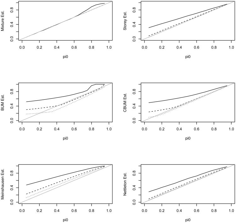
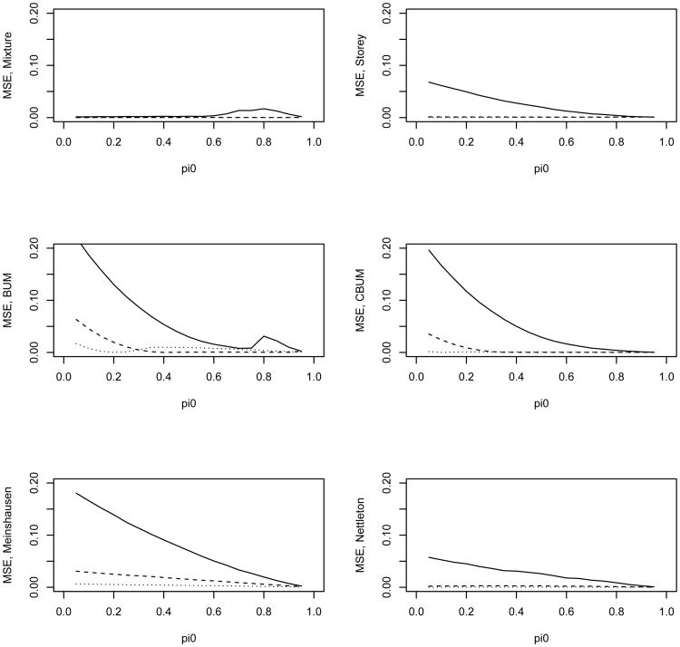
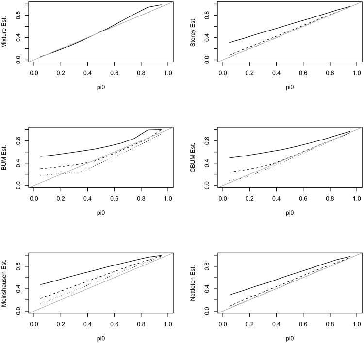
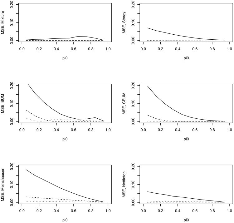
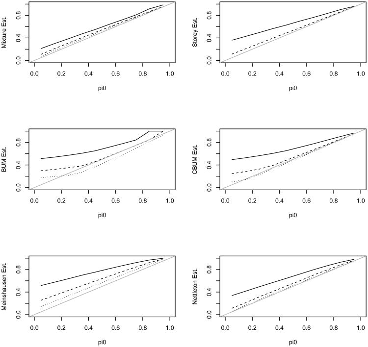
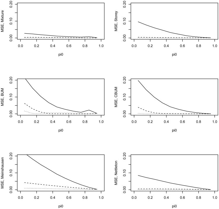
We first simulated the independent case in which all the tests from either the null or the alternative hypothesis were independent from each other. Figures 2–3 present the estimate of π₀ and its mean squared error (MSE) for the 6 methods. The estimates were averaged over 200 simulation replicates each with a sample size N = 5,000. Figure 2 shows that the distribution mixture-based estimate (denoted as the mixture estimate) agrees with the true value better than the other methods. Figure 3 shows the MSE for these estimates. Except for λ = 4 and 0.8 < π₀ < 0.95, the mixture estimate clearly performs better than the other five methods. In the top left panel of Figure 2 the dashed and dotted lines almost overlay the true value line indicating that the mixture estimate of π₀ is almost identical with the true values for the two scenarios with λ = 6 or λ = 9. In addition, the mixture estimate provides an excellent estimate of λ (due to space limitation, the estimate of λ is not reported; it is available from the corresponding author upon request). Only for λ = 4 and 0.8 < π₀ < 0.95, the other methods have comparable or slightly better performance than the mixture estimate. We next examine why our estimate seemed to overestimate π₀ for these scenarios.

Figure 2.

Estimated π₀ using the 6 different methods versus the true π₀. The solid, dashed, and dotted lines are for λ value of 4, 9, and 16 in the alternative, respectively. The tests are independent from each other. Note, the mixture estimate is almost identical with the true π₀ for λ value of 9 and 16.

Figure 3.

MSE of the estimated π₀ versus the true π₀ for the 6 different methods. The solid, dashed, and dotted lines are for λ value of 4, 9, and 16 in the alternative, respectively. The tests are independent from each other.

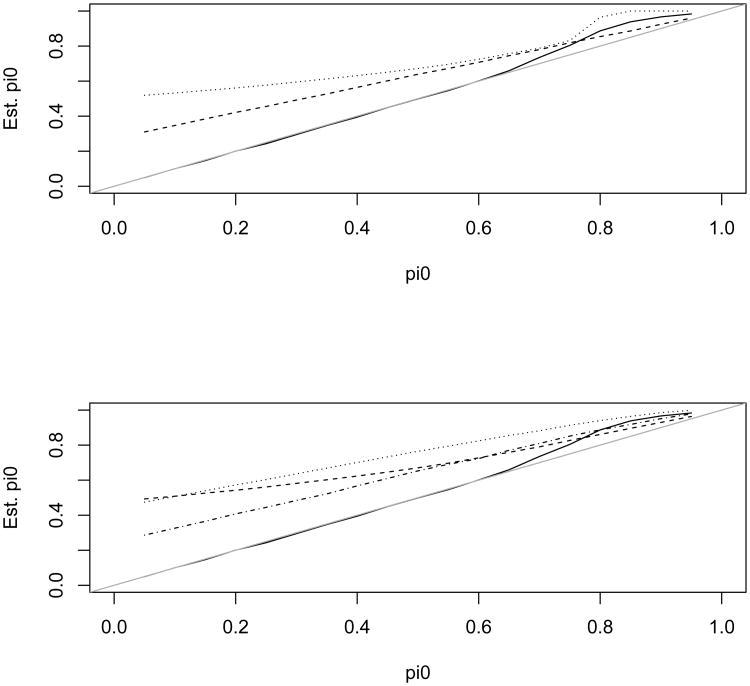
The estimates (average over 200 simulation replicates) of π₀ for λ = 4 are shown in Figure 4. A closer examination of the 200 estimates showed that the mixture estimate had difficulty in estimating the small percentage from the alternative for a fraction of the simulated datasets. These datasets resulted to λ̂ = 0 and π̂₀ = 1. Unfortunately in these time-consuming simulations, we just had to take π̂₀ = 1 as the estimate for these simulation replicates and this caused the average to overestimate π₀ and underestimate λ. Xiang, Edwards, and Gadbury (2006) encountered similar difficulties in their simulations. We only observed this for λ = 4, but not for λ = 9 or 16. Nevertheless, the mixture estimate was still comparable with the other estimates in this parameter range. This observation suggests the closeness of the alternative component to the uniform also plays a role in estimating the parameters.

Figure 4.

Estimated π₀ using the 6 different methods versus the true π₀ for λ = 4 in the alternative. Top graph: the solid, dashed, and dotted lines are for the mixture, Storey, and BUM estimates, respectively; Bottom graph: the solid, dashed, dotted, and dash-dotted lines are for the mixture, CBUM, Meinshausen, and Nettleton estimates, respectively.

In the simulations, we used 10 for λ and the estimate of π₀ by the threshold method of Storey and Tibshirani (2003) as the initial values in our method. In real data analysis, we could start with these initial values. If the resulted estimates are λ̂ = 0 and π̂₀ = 1, it would suggest: 1) the fitted model will not fit well on the observed p-value histogram; and 2) π₀ is close to 1 and λ is small. We can then choose the initial parameters and visually examine the “best-guess” mixture model against the observed p-value histogram as shown in Figure 10. R routine nlm conducts the minimization using a Newton-type algorithm. In the above scenario, the resulted λ̂ = 0 and π̂₀ = 1 also suggests the likelihood in the neighborhood of (λ = 0, π₀ = 1) is fairly flat. In the nlm routine, we can adjust the argument gradtol, which specifies the tolerance at which the scaled gradient is considered close enough to zero to terminate the algorithm. In addition, one should always check the eigenvalues of the final Hessian matrix. Since nlm is to minimize the negative log likelihood, both eigenvalues should be positive. If there are zero or negative eigenvalues, it would suggest a questionable fit. By fine-tuning the arguments in the routine and using the “best-guess” initial values, we found the algorithm can converge to reasonable estimates of π₀, i.e. away from the boundary π̂₀ = 1 that tends to overestimate π̂₀. R routine nlm has a set of arguments and detailed explanations can be found in the R help file and the original references cited therein if readers need to learn more about the algorithm to fit their data.

When π₀ approaches 1, and the alternative is close to the null, e.g. λ = 4, the simulations seem to suggest the threshold method of Storey and Tibshirani (2003) provide a slightly better alternative to estimating π₀ before our method could be fine-tuned as above to obtain the estimate. This is consistent with simulations conducted by Li, Bigler et al. (2005). There is a theoretical reason for this observation and we will comment on this further in the discussion section.

4.3. Simulation scenario 2: there are clusters of correlated tests

In real data analysis, correlations are often present in clusters of genes. We used the following additive property of the chi-squared distribution to introduce correlations within clusters of tests in the simulations. Suppose independent random variables X and Z follow non-central chi-squared distribution ${\chi }_{{\lambda }_1}^2(n_1)$ and ${\chi }_{{\lambda }_2}^2(n_2)$, respectively, their sum X + Z follows non-central chi-squared distribution ${\chi }_{{\lambda }_1+{\lambda }_2}^2(n_1+n_2)$ with non-centrality parameter λ₁ + λ₂ and n₁ + n₂ df. For the j^th test within cluster i, let Y_ij = X_ij + Z_i where $X_{ij}~{\chi }_{{\lambda }_{ij}}^2(n_{ij})$ are independent from each other and they are also independent from a cluster-level random effect $Z_i~{\chi }_{{\lambda }_i}^2(m_i)$. This set-up introduces a correlation

$$\text{Corr}(Y_{ij},Y_{i{j}^{\prime }})=(m_i+2{\lambda }_i)/{(n_{ij}+m_i+2({\lambda }_{ij}+{\lambda }_i))}^{1/2}{(n_{i{j}^{\prime }}+m_i+2({\lambda }_{i{j}^{\prime }}+{\lambda }_i))}^{1/2}$$

among the test statistics within the cluster, where X_ij′ follows ${\chi }_{{\lambda }_{i{j}^{\prime }}}^2(n_{i{j}^{\prime }})$ distribution.

Figures 5 and 6 present the estimates of π₀ and their MSE for scenarios with modest correlation within clusters of 30 tests. To introduce the correlation, we set the cluster-level random effect Z_i ∼ χ²(4) and $Z_i~{\chi }_3^2(4)$ for tests in the null and in the alternative hypothesis, respectively. The distribution of X_ij is set accordingly to maintain the test statistic Y_ij at ν = 10 df with non-centrality parameter of λ = 4, 9, or 16 in the alternative. This results to a within-cluster correlation coefficient of 0.4 between the test statistics for tests under the null and correlation coefficients of 0.56, 0.36, 0.24 for tests under the alternative with λ = 4, 9, 16, respectively. For each simulation, 30% of the tests are in clusters of size 30 and the other 70% of the tests are independent from each other and from the tests in the clusters. Figures 5 and 6 essentially show a similar pattern as that shown in the estimates for the independent case. In general, the mixture estimate performed better than the others. The MSE of the mixture estimate slightly increased in the presence of within-cluster correlations. However, it is still much smaller than the MSE of the other estimates for a broad range of π₀. We also simulated scenarios with weaker or stronger within-cluster correlations. The estimates behaved similarly in those scenarios, and the results are not included in this report.

Figure 5.

Estimated π₀ using the 6 different methods versus the true π₀. The solid, dashed, and dotted lines are for λ value of 4, 9, and 16 in the alternative, respectively. The correlation coefficient is 0.4 between test statistics within a cluster for tests under the null and the correlation coefficients are 0.56, 0.36, 0.24 for tests under the alternative with λ = 4, 9, 16, respectively.

Figure 6.

MSE of the estimated π₀ versus the true π₀ for the 6 different methods. The solid, dashed, and dotted lines are for λ value of 4, 9, and 16 in the alternative, respectively. The correlation coefficient is 0.4 between test statistics within a cluster for tests under the null and the correlation coefficients are 0.56, 0.36, 0.24 for tests under the alternative with λ = 4, 9, 16, respectively.

4.4. Simulation scenario 3: there are multiple components in the alternative

In the above simulations, we assumed there was one alternative hypothesis represented by the non-centrality parameter λ. In real data analysis, the alternative could be from a range of alternatives represented by different corresponding values of λ. This would naturally lead us to consider a multicomponent mixture model. However, estimating the number of components in a mixture is a difficult unresolved problem (McLachlan and Peel, 2000, page 175). In the case of multiple hypotheses testing when the alternative hypothesis is true for many of them, each of the alternative hypotheses could be unique. This further increases the difficulty in modeling them as a mixture of a finite number of alternatives. In the p-value mixture model, this implies that we actually have a class of distributions ψ(p | λ) indexed by λ. When we fit the two-component mixture model (5), the non-null component is actually an average of the many ψ(p | λ)'s.

To evaluate the impact of this multicomponent mixture on the various estimates of π₀, we conducted additional simulations. The simulation was set up with the similar correlation structure as the above single-alternative case but now the alternative was a mixture of three components (λ = 4, 6, 9) with weights (0.3, 0.3, 0.4). Then we fit the two-component mixture model (5) and we also estimated π₀ using the other 5 methods. The estimates are presented in Figure 7. The estimate of π₀ using our model was comparable with the other methods, demonstrating a similar robustness to the non-parametric methods.

Figure 7.

Estimated π₀ from the 6 different methods versus the true π₀ for a mixture in the alternative. Top graph: the solid, dashed, and dotted lines are for the mixture, Storey, and BUM estimates, respectively; Bottom graph: the solid, dashed, dotted, and dash-dotted lines are for the mixture, CBUM, Meinshausen, and Nettleton estimates, respectively.

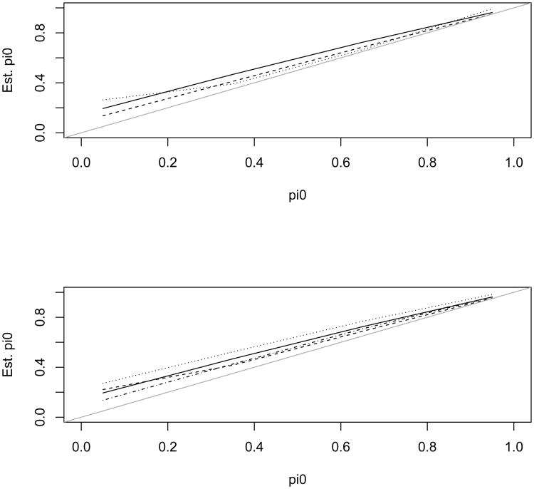
We also conducted simulation studies to evaluate the estimate of π₀ when model (4) is mixed with the uniform. This continuous mixture model represents a range of alternatives with their corresponding λ sampled from Gamma (k, θ) distribution. We chose k = 4, 9, 16 and θ = 0.5. Unfortunately we ran into an identifiability problem with model (4). We took a step back to fit the (mis-specified) two-component mixture of uniform and model (3). Along with the other 5 methods the estimates of π₀ are presented in Figure 8 and their MSE are presented in Figure 9. These simulations show that our estimate has favorable performance than the other methods, parametric or nonparametric, in this setting. The estimated λ is generally slightly larger than twice of kθ, the mean of the Gamma (k, θ) distribution.

Figure 8.

Estimated π₀ using the 6 different methods versus the true π₀. The solid, dashed, and dotted lines are for λ sampled from Gamma (k, θ) with k = 4, 9, 16, respectively, and θ = 0.5 in the alternative.

Figure 9.

MSE of the estimated π₀ versus the true π₀ for the 6 different methods. The solid, dashed, and dotted lines are for λ sampled from Gamma (k, θ) with k = 4, 9, 16, respectively, and θ = 0.5 in the alternative.

These identifiability difficulties are perhaps one of the main contributors to the current state that works in this area almost always assume there is one alternative even though a multicomponent alternative is more plausible. Yet in this simplified setting of misspecified models, the estimate based on the mixture of uniform and (3) offers a favorable performance in estimating π₀. We attribute this gain to the application of the appropriately derived distribution (3) in the mixture model.

5. Example: Gene expression in anti-IgM antibody-treated MZ B cells in MALT lymphoma

The B-cell lymphoma/leukemia-10 (BCL10) protein is believed to have important tumorigenic effects on mucosa-associated lymphoid tissue (MALT) lymphomas (Zhang, Siebert et al., 1999 and Pounds and Morris, 2003). A microarray gene expression study was conducted at St. Jude Children's Hospital in Memphis, Tennessee. The marginal zone (MZ) B lymphocytes from two types of mice were purified, then either treated with an anti-IgM antibody or not treated; the not-treated served as controls. The mice are transgenic FVB strain mice engineered to over-express BCL10 in their B cells or wild-type FVB mice. Gene expressions were measured under the four experimental conditions defined by the two factors. Eight array measurements were obtained using the wild-type, non-anti-IgM-activated MZ B-cells; ten from the BCL10-over-expressing, non-anti-IgM-activated MZ B cells; seven from the wild-type, anti-IgM-activated MZ B cells; and four from the BCL10-over-expressing, anti-IgM-activated MZ B cells. The Kruskal-Wallis test was conducted to compare all four groups due to a lack of normality of the expression values. A p-value was obtained for each of the 12,488 probes using the chi-squared test with 3 df. The dataset of p-values was generously provided to us by Dr. Stanley Pounds. More details about the study and an initial analysis can be found in Pounds and Morris (2003).

We applied the six methods evaluated in Section 4 to these 12,488 p-values. The histogram along with the fitted model (5) and the BUM model of Pounds and Morris (2003) are presented in Figure 10. Both models seem to fit well to the observed p-value histogram. Estimates of π₀ from the six methods are in Table 1. The estimates of the parameters using the mixture model (5) are π̂₀ = 0.5358 (95% CI (0.5184, 0.5532)) and λ̂ = 6.99 (CI (6.74, 7.25)). Simulation studies in Section 4 suggest that the mixture estimate of π₀ should be preferred to other estimates for parameters in this range. None of the other 5 methods provides CI for π̂₀ in their R packages. We obtained the bootstrap CI for two of them and for the other three the CI is not calculated since the estimate itself is an upper-bound of π₀. The mixture estimate π̂₀ has the narrowest CI among the three CI's reported in Table 1.

We also fit model (5) using gamma mixture of Poisson model (4) for the distribution of P which accounts for a range of alternatives. We used four sets of initial values of (π₀, k, θ) to numerically obtain their MLE's. The estimate π̂₀ was always 0.5357. The estimate k̂ was in the range of 4,034 to 164,284, and the corresponding estimate θ̂ was in the range of 8.67 × 10⁻⁴ to 2.13 × 10⁻⁵, while the product k̂θ̂ remains a constant 3.495. These estimates indicate the negative binomial distribution NB (k, θ/(1 + θ)) has a constant mean k̂θ̂ = 3.495 as k̂ varies for different fit. Its variance is kθ(1 + θ) and the extremely small estimates of θ indicate barely any over-dispersion. In this dataset, the negative binomial distribution converges to Poisson (3.495). Note λ̂ = 6.99 using model (3) is twice of 3.495 since we assumed U = λ/2 follows the Gamma (k, θ) distribution. These fits result to almost identical distribution curves as that of the two-component mixture model (5) with π̂₀ = 0.5358 and λ̂ = 6.99. These results suggest an identifiability issue for (k, θ) when fitting the continuous gamma mixture model (4) to this dataset. We conducted additional simulation studies that indicate the identifiability of k and θ is an issue for the gamma mixture of Poisson model (4). This identifiability issue reflects a long-standing difficulty in identifying multi-component in mixtures, e.g. as in a comment by McLachlan and Peel (2000, page 175) that estimating the number of components in a mixture is a difficult unresolved problem. Further research on this topic is needed to help us move beyond the two-component mixtures, even though our method performs reasonably well in this misspecified setting as demonstrated in the simulation studies in Section 4.4.

The analysis results indicate that 53.6% of the p-values were from the null hypothesis. This means in 46.4% of the genes at least one of the four groups had a different mean expression. This 46.4% seems to be excessive, but it is the second lowest estimate among the six methods. The only lower estimate of 45.5% by the method of Meinshausen and Rice (2006) is actually a lower bound of the proportion of differentially expressed genes. All these estimates seem to be high, however, as Pounds and Morris (2003) point out, “this fraction includes any gene that is even slightly differentially expressed in any of the four treatments.” Our estimate of λ̂ = 6.99 provides an estimate of the magnitude of the difference. More comments on how to interpret the proportion of a seemingly excessively large number of genes under the alternative can be found in Pounds and Morris (2003) and Efron (2004).

6. Discussion

Estimating the proportion π̂₀ has attracted a significant amount of research, especially in the nonparametric framework (Broberg, 2005; Langaas, Lindqvist, and Ferkingstad, 2005; Cheng, 2006; Nettleton et al., 2006; Meinshausen and Rice, 2006; Tang, Ghosal, and Roy, 2007). These methods attempt to estimate π₀ without using a parametric distribution for the p-values under the alternative, ψ(p), in the two-component mixture model (1). Identifiability of π₀ has been a long-standing difficulty.

We approach the problem from a different angle by deriving a parametric distribution for p-values under the alternative. The derived distribution enables us to fit the two-component mixture model (1) to the observed p-values. The second component depends on the specific test that is used to obtain the p-values. As long as the non-null component ψ(p) is not reproduced when mixed with the uniform, the mixing proportion π₀ and the non-null component ψ(p) can be estimated using the maximum likelihood method. Langaas, Lindqvist, and Ferkingstad (2005) and Tang, Ghosal, and Roy (2007) set restrictions such as ψ(1) = 0 to solve the identifiability problem. For the chi-squared test, our derived ψ(p) shows that ψ(1) = e^−λ/2 is not zero.

In simulation studies, our method performed favorably in comparison with 5 recent methods for a broad range of scenarios including scenarios with clusters of correlated tests, multicomponent alternative mixtures, and continuous alternative mixture in which λ follows Gamma(k, θ) distribution. However, as one would expect, when π₀ approached one and the alternative was close to the null, our method also had difficulty estimating the proportion. In this situation, it appeared that the threshold method of Storey and Tibshirani (2003) slightly outperformed the other methods. In Appendix B, we derive the bias in the estimate of the threshold method. The bias can be expressed as m(1 – π₀)[1 – Ψ(α)]/(1 – α), where Ψ(·) is the cumulative distribution function for ψ given in (9) and m is the total number of hypotheses being tested. This bias goes to zero when π₀ approaches one. Thus, we recommend that users may want to use the threshold method to estimate π₀ in this situation. However, the threshold method loses the ability to estimate the non-null effect λ. The method was developed to exploit the fact that p-values under the null are uniformly distributed, and the distribution of the truly alternative p-values can not be specified (Storey and Tibshirani, 2003, page 9442). The estimate of λ informs us where on average the alternative is when we interpret π̂₀. It provides useful information especially when 1 – π̂₀ appears to be excessive as in the example in Section 5.

Appendix A. Derivation of distribution ψ

Under the null hypothesis H₀, for any 0 < p < 1 the reported “p-value” of the statistical test based on X has cumulative distribution

$$Pr[\mathrm{p}-\text{value}\le p|H_0]={\int }_{x_{1-p}}^{\infty }f(x)dx=p.$$

This is the well known result that the p-value has a uniform distribution under the null hypothesis.

Under a specified alternative hypothesis H_a suppose the test statistic X follows the cumulative distribution G(·) with density function g(·). Then for any0 < p < 1

$$Pr[\mathrm{p}-\text{value}\le p|H_a]={\int }_{x_{1-p}}^{\infty }g(x)dx=1-G(x_{1-p}).$$ (8)

Let ψ(p) = ψ(p | H_a) denote the density function corresponding to the distribution at (8). Then

$$\begin{array}{c}\psi (p)=-(\partial /\partial p)G(x_{1-p})\\ =-g\{F^{-1}(1-p)\}(\partial /\partial p)F^{-1}(1-p)\\ =g(x_{1-p})/f(x_{1-p})\end{array}$$ (9)

or the likelihood ratio evaluated at the upper p–th quantile of F.

The density function of a non-central chi-squared distribution with ν df and non-centrality parameter λ ≥ 0 can be expressed as a weighted sum of a central chi-squared density with the probabilities of a Poisson distribution with mean λ/2 as the weights

$$g(x|\lambda )=\sum _{j=0}^{\infty }\{\frac{{(\lambda /2)}^j}{j!}{e}^{-\lambda /2}\}f(x;\nu +2j)$$

(c.f. Johnson, Kotz, and Balakrishnan, 1995, p436, and Fisher, 1928) from which (9) evaluates to

$$\psi (p)=\sum _{j=0}^{\infty }\left\{\frac{{(\lambda /2)}^j}{j!}{e}^{-\lambda /2}\right\}\frac{f(x_{1-p};\nu +2j)}{f(x_{1-p};\nu )}=\sum _{j=0}^{\infty }\left\{\frac{{(\lambda /2)}^j}{j!}{e}^{-\lambda /2}\right\}\frac{\mathrm{\Gamma }(\nu /2)}{\mathrm{\Gamma }(\nu /2+j)}{(x_{1-p}/2)}^j=e^{-\lambda /2}+\sum _{j=1}^{\infty }\left\{\frac{{(\lambda /2)}^j}{j!}{e}^{-\lambda /2}\right\}\frac{x_{1-p}^j}{(\nu +2j-2)(\nu +2j-4)\cdots \nu },$$ (10)

where x_1–p is the upper 1 – p quantile of a (central) chi-squared random variable with ν df.

It is trivial to prove that the likelihood ratio f(x_1–p; ν + 2j)/f(x_1–p; ν) in (10) satisfies the monotone likelihood ratio property (MLRP) (see Ferguson, 1967, page 208, for example). Along with the derivative (∂/∂p)x_1–p = –f(x_1–p), this MLRP guarantees ψ(p) is a monotone decreasing function in p. This is a desired property and it has been assumed by Langaas, Lindqvist, and Ferkingstad (2005) and Tang, Ghosal, and Roy (2007) in their nonparametric modeling of distributions for p-values.

Next we consider a reference statistic that results in a beta distribution for ψ. Suppose F(·) and G(·) differ by a Lehmann alternative through their survival functions. This class includes the exponential distribution as a special case and also proportional hazards models, but not all of the distributions in the exponential family. Specifically, let S(x) = 1 – F(x) denote the survival function corresponding to F under the null hypothesis and suppose 1–G(x) = {S(x)}^1–δ for some 0 < δ < 1 under the alternative.

Then ψ at (9) satisfies

$$\psi (p)=(1-\delta )p^{-\delta }.$$

This is a beta density with parameters α = 1 – δ and β = 1.

Appendix B. Bias in the estimate of π₀ by the threshold method of Storey and Tibshirani (2003)

We use the same notations as those used by Benjamini and Hochberg (1995) in a multiple hypotheses testing problem. Table 2 illustrates the model.

Table 2.

Testing m hypotheses among which m₀ null hypotheses and m₁ alternative hypotheses are true.

Truth	Reject H0		total
	No	Yes
H0	U	V	m0
Ha	T	S	m1
	m–R	R	m

Let R(α) be the number of rejections at significance level α. Given that the right margin in Table 2 is fixed, the random variables V and S follow binomial distributions. V ∼ Bin(m₀, α) and S ∼ Bin(m₁, Ψ(α)), where Ψ(α) is the cumulative distribution function for ψ given in (9). We have R = V + S with expectation

$$\mathrm{E}R(\alpha )=m_1\Psi (\alpha )+m_0\alpha .$$

Then we have

$$m-\mathrm{E}R(\alpha )=m_1[1-\Psi (\alpha )]+m_0(1-\alpha ).$$

Schweder and Spjoetvoll (1982) use the least squares estimate of the slope in regression

$$m-R(\alpha )\approx m_0(1-\alpha )$$

to estimate m₀. The slope has an expectation of m₀ + m₁[1 – Ψ(a)]/(1 – a). This slope estimate of m₀ has a bias m₁[1 – Ψ(α)]/(1 – α) = m(1 – π₀)[1 – Ψ(α)]/(1 – α). The bias decreases as Ψ(α) → 1 or when m₁ is small relative to m₀.

References

- Allison DB, Gadbury GL, Heo M, Fernandez JR, Lee CK, Prolla TA, Weindruck R. A mixture model approach for the analysis of microarray gene expression data. Computational Statistics & Data Analysis. 2002;39:1–20. [Google Scholar]
- Benjamini Y, Hochberg Y. Controlling the false discovery rate: A practical and powerful approach to multiple testing. Journal of the Royal Statistical Society B. 1995;57:289–300. [Google Scholar]
- Benjamini Y, Hochberg Y. On the adaptive control of the false discovery rate in multiple testing with independent statistics. Journal of Educational and Behavioral Statistics. 2000;25:60–83. [Google Scholar]
- Broberg P. A comparative review of estimates of the proportion unchanged genes and the false discovery rate. BMC Bioinformatics. 2005;6:199–218. doi: 10.1186/1471-2105-6-199. [DOI] [PMC free article] [PubMed] [Google Scholar]
- Cheng C. An adaptive significance threshold criterion for massive multiple hypotheses testing. IMS Lecture Notes–Monograph Series, 2nd Lehmann Symposium – Optimality. 2006;49:51–76. [Google Scholar]
- Diaconis P, Ylvisaker D. Quantifying Prior Opinion. Bayesian Statistics 2: Proceedings of the Second Valencia International Meeting; September 6/10, 1983; Amsterdam & New York: North-Holland & Valencia University Press; 1985. pp. 133–156. 1985. [Google Scholar]
- Efron B, Tibshirani R, Storey JD, Tusher V. Empirical Bayes analysis of a microarray experiment. Journal of the American Statistical Association. 2001;96:1151–1160. [Google Scholar]
- Efron B, Tibshirani R. Empirical Bayes methods and false discovery rates for microarrays. Genet Epidemiol. 2002;23:70–86. doi: 10.1002/gepi.1124. [DOI] [PubMed] [Google Scholar]
- Efron B. Large-scale simultaneous hypothesis testing: the choice of a null hypothesis. Journal of the American Statistical Association. 2004;99:96–104. [Google Scholar]
- Ferguson TS. Mathematical Statistics: A Decision Theoretic Approach. New York: Academic Press; 1967. [Google Scholar]
- Fisher RA. The general sampling distribution of the multiple correlation coefficient. Proceedings of the Royal Society of London. 1928 Dec 1;121(788):654–673. Series A, Containing Papers of a Mathematical and Physical Character. 1928. [Google Scholar]
- Johnson L, Kotz S, Balakrishnan N. Continuous Univariate Distributions. Second. Vol. 2. New York: J. Wiley & Sons; 1995. [Google Scholar]
- Kruskal WH, Wallis A. Use of ranks in one-criterion variance analysis. Journal of the American Statistical Association. 1952;47:583–621. [Google Scholar]
- Langaas M, Lindqvist BH, Ferkingstad E. Estimating the proportion of true null hypotheses, with application to DNA microarray data. Journal of the Royal Statistical Society B. 2005;67:555–72. [Google Scholar]
- Li SS, Bigler J, Lampe JW, Potter JD, Feng Z. FDR-controlling testing procedures and sample size determination for microarrays. Statistics in Medicine. 2005;24:2267–2280. doi: 10.1002/sim.2119. [DOI] [PubMed] [Google Scholar]
- Markitsis A, Lai Y. A censored beta mixture model for the estimation of the proportion of non-differentially expressed genes. Bioin-formatics. 2010;26:640–646. doi: 10.1093/bioinformatics/btq001. [DOI] [PMC free article] [PubMed] [Google Scholar]
- McLachlan GJ, Peel D. Finite Mixture Models. Chapter 6. New York: J. Wiley & Sons; 2000. p. 175. [Google Scholar]
- Meinhausen N, Rice J. Estimating the proportion of false null hypotheses among a large number of independently tested hypotheses. Annals of Statistics. 2006;34:373–393. [Google Scholar]
- Nettleton D, Hwang J, Caldo RA, Wise RP. Estimating the number of true null hypotheses from a histogram of p values. J Agric Biol Environ Stat. 2006;11:337–356. [Google Scholar]
- Parker RA, Rothenberg RB. Identifying important results from multiple statistical tests. Statistics in Medicine. 1988;7:1031–43. doi: 10.1002/sim.4780071005. [DOI] [PubMed] [Google Scholar]
- Pounds S, Morris SW. Estimating the occurrence of false positives and false negatives in microarray studies by approximating and partitioning the empirical distribution of p-values. Bioinformatics. 2003;19:1236–42. doi: 10.1093/bioinformatics/btg148. [DOI] [PubMed] [Google Scholar]
- Schweder T, Spjoetvoll E. Plots of P-values to evaluate many tests simultaneously. Biometrika. 1982;69:493–502. [Google Scholar]
- Storey JD, Tibshirani R. Statistical significance for genomewide studies. PNAS. 2003;100(16):9440–9445. doi: 10.1073/pnas.1530509100. [DOI] [PMC free article] [PubMed] [Google Scholar]
- Tang Y, Ghosal S, Roy A. Nonparametric Bayesian estimation of positive false discovery rates. Biometrics. 2007;63:1126–34. doi: 10.1111/j.1541-0420.2007.00819.x. [DOI] [PubMed] [Google Scholar]
- Xiang Q, Edwards J, Gadbury G. Interval estimation in a finite mixture model: Modeling p-values in multiple testing applications. Computational Statistics & Data Analysis. 2006;51:570–586. [Google Scholar]
- Zhang Q, Siebert R, et al. Inactivating mutations and overexpression of BCL10, a caspase recruitment domain-containing gene, in MALT lymphoma with t(1;14)(p22;q32) Nat Genet. 1999;22:63–68. doi: 10.1038/8767. [DOI] [PubMed] [Google Scholar]