

Abstract
Cancer is a complex, multiscale process, in which genetic mutations occurring at a subcellular level manifest themselves as functional and morphological changes at the cellular and tissue scale. The importance of interactions between tumour cells and their microenvironment is currently of great interest in experimental as well as computational modelling. Both the immediate microenvironment (e.g. cell–cell signalling or cell–matrix interactions) and the extended microenvironment (e.g. nutrient supply or a host tissue structure) are thought to play crucial roles in both tumour progression and suppression. In this paper we focus on tumour invasion, as defined by the emergence of a fingering morphology, which has previously been shown to be dependent upon harsh microenvironmental conditions. Using three different modelling approaches at two different spatial scales we examine the impact of nutrient availability as a driving force for invasion. Specifically we investigate how cell metabolism (the intrinsic rate of nutrient consumption and cell resistance to starvation) influences the growing tumour. We also discuss how dynamical changes in genetic makeup and morphological characteristics, of the tumour population, are driven by extreme changes in nutrient supply during tumour development. The simulation results indicate that aggressive phenotypes produce tumour fingering in poor nutrient, but not rich, microenvironments. The implication of these results is that an invasive outcome appears to be co-dependent upon the evolutionary dynamics of the tumour population driven by the microenvironment.
1 Introduction
Fingering and branched patterns can be found in a variety of animate [15] and in-animate [47] systems. One large class of non-living systems that exhibit fingering patterns are those obeying diffusion limited growth. In this growth process the interface between two phases is advanced at a rate proportional to the gradient of a potential field u that obeys Laplace equation ∇2u = 0 in one phase and satisfies the boundary condition u = 0 at the interface and in the other phase. Depending on the system under consideration the field u represents different physical quantities. In viscous fingers [29] it is the pressure in the liquid, in electro-chemical deposition [56] it is the electrical field around the substrate and in crystal growth it is the temperature [16]. The growth instabilities that occur in these systems are described by the Mullins–Sekerka instability [60], which shows that the typical length scale of the pattern depends on microscopic parameters of the system under consideration.
Morphologies similar to those encountered in diffusion limited growth can be observed in microbial colonies during stressed growth conditions, such as low nutrient concentration or elevated substrate stiffness. When the nutrient concentration is increased the morphology becomes more compact and lowering the substrate stiffness leads to a smoother colony boundary [55,57]. Fungal growth is an example of another biological system in which fingering morphologies arise in low nutrient concentrations when there is a buildup of metabolites that inhibit growth [51]. It is interesting to note that in both examples the finger-like morphology does not seem to arise due to cell cooperation, but rather emerges from the underlying physical properties of the microenvironment.
A commonly accepted biological view is that tumour invasion is associated with the capability of cells to break free from the primary tumour mass into the adjacent tissue, since this capability may be considered as a first step toward metastasis [42,66,50]. Such fragmentation of cancer tissue is usually an indication of a high grade tumour as determined by the TNM system [90] and can be observed in pathological specimens [36,54]. Thus, the irregular, finger-like margins or completely disconnected cohorts of tumour cells are characteristic of aggressive tumours as opposed to more benign tumours which are characterised by smooth non-invasive margins.
Such different types of morphologies have been observed in several models of tumour growth, and again the growth patterns seem to be driven by the microenvironment. Ferreira et al. [35] presented a hybrid reaction–diffusion model of tumour growth, where two types of nutrients were considered—one essential and one nonessential for cell proliferation, and upon varying the consumption rate of the essential nutrient their model exhibited a variety of morphologies, ranging from compact, fingered to disconnected. The impact of the extracellular matrix (ECM) on tumour morphology was investigated by Anderson using a hybrid–discrete–continuous model [5,12]. He showed that growth in a heterogeneous ECM gives rise to a fingered morphology and, moreover, that such a morphology can also be induced by lowering the oxygen concentration in a homogeneous ECM, highlighting the importance of oxygen availability in determining tumour structure. Anderson also established a link between the tumour morphology and the phenotypes of individual tumour cells which was subsequently refined by Gerlee and Anderson [40] using an evolutionary hybrid cellular automata model that considered the genotype to phenotype mapping using a neural network. This work also linked low nutrient availability with a fingered tumour morphology, and showed that tumours with irregular shapes are more likely to contain aggressive phenotypes. A further model that considered individual deformable elastic cells interacting with a surrounding fluid and nutrients has been used by Rejniak in [75,76]. She showed that the emergence of tumour microregions characterised by different cell subpopulations and distinct nutrient concentrations subsequently leads to the formation of finger-like tumour morphologies where long tissue extensions are created as a result of cell competition for resources in the tumour vicinity. When the finger-like morphology is coupled with the development of necrotic areas, the fingering effectively results in fragmentation of the primary tumour into several independent invasive colonies.
The importance of the tumour microenvironment is currently of great interest to both the biological and the modelling communities. In particular, both the immediate microenvironment (e.g. cell–cell signalling or cell–matrix interactions) and the extended microenvironment (e.g. vascular bed or nutrient supply) are thought to play crucial roles in both tumour progression and suppression (see the recent series of papers in Nature Reviews Cancer for further detail [2,17,63]). Recently it has been shown that not only can the microenvironment promote tumour progression but it can also drive the invasive tumour phenotype. The work of Weaver [64] focuses on the impact of tissue tension in driving the invasive phenotype and clearly correlates higher tension in the tissue (a harsher environment) with an invasive phenotype. Similarly Pennacchietti [67] has shown a relationship between a hypoxic tumour microenvironment (again a harsher environment) and the invasive phenotype. Höckel et al. [44] also showed in a study on cervical cancers that hypoxic tumours in general exhibited larger tumour extensions compared to non-hypoxic ones.
2 Modelling overview
Over the last 10 years or so many mathematical models of tumour growth, both temporal and spatio-temporal, have appeared in the research literature (see [14,73] for a review). Deterministic reaction–diffusion equations have been used to model the spatial spread of tumours in the form of invading travelling waves of cancer cells [26,27,39,62,68,84,87,89]. The cumulative growth of tumours has also been modelled with partial differential equations solved using various numerical simulation techniques, such as boundary-integral, finite-element and level-set methods [28,53,93]. Whilst all these models are able to capture the tumour structure at the tissue level, they fail to describe the tumour at the cellular level. On the other hand, single-cell-based models provide such a description and allow for a more realistic stochastic approach at both the cellular and subcellular levels. Several different discrete models of tumour growth have been developed recently, including cellular automata models [1,31,33,46,65,74,85], Potts models [45,82,88], lattice free cell-centered models [32] or agent-based models [92]. For a review on many different single-cell-based models applied to tumour growth and other biological problems please see [9].
Here we will present three different examples of such single-cell-based tumour growth models classified as “hybrid”, since a continuum deterministic model controls the environmental dynamics (e.g. nutrient, ECM or chemical) whereas the cell life processes of proliferation and death, mutation, cell–cell interactions and migration will be handled at a discrete individual cell level. The three models we conisder are: (1) a Hybrid Discrete-Continuum (HDC) model which couples a system of reaction–diffusion equations to model the dynamics of nutrients, the extracellular matrix and matrix-degradative enzymes with a discrete cellular automata like model based on a biased random-walk technique [4,5,7,8,10-12]; (2) an Evolutionary Hybrid Cellular Automata (EHCA) model which is an extension of the cellular automaton in which each cell is equipped with a response network that determines the cellular behaviour from environmental variables using a feed-forward artificial neural network [40]; (3) an Immersed Boundary (IBCell) model which couples the dynamics of viscous incompressible fluid with the mechanics of individual fully deformable elastic cells that interact with one another and with their microenvironment via a set of discrete cell membrane receptors located on cell boundaries [75-77,80,81].
In all three models we represent the microenvironment of an individual cell in a very simplified way by including only neighbouring tumour cells and one external diffusive factor. This may seem like an oversimplification since in reality tumours may be surrounded by stromal cells and may be exposed to different nutrients, growth factors and various proteases that all together influence changes in cell behaviour. However, as we want to focus on internal cell properties (transformations in cell phenotype and genotype, dynamical reorganisation of cell membrane receptors, changes in cell response due to switches in nutrient supply) we therefore choose to represent the extracellular matrix in all three models in a unified simple way. For the same reason, we decided to use oxygen as the basic external factor that creates a competitive environment and influences cell response, but oxygen could be exchanged for another nutrient, e.g. glucose. An advantage in choosing oxygen is that its value can be manipulated in the course of an in vitro biological experiment, and this is, of course, much easier to do in the in silico simulations presented here.
Each model uses a distinct mechanism for the selection of cell phenotypes in response to environmental cues (such as oxygen concentration and contact with neighbouring cells), but all three are not only able to couple the behaviour of individual tumour cells with the continuous nutrient dynamics, but they also explicitly incorporate the impact of the microenvironment upon both the tumour morphology and tumour heterogeneity. By using a combination of different microenvironments (e.g. low/high nutrient concentration) with different cell properties (i.e. random or evolutionary mutations, local receptor driven or mean-field response to nutrients) we will show how aggressiveness of a tumour and the formation of finger-like invasive tissue extensions are linked and how these correlate with the microenvironment in which the tumour grows.
3 Nutrient driven invasion: model descriptions
Our goal is to investigate how the microenvironment of a growing tumour influences its invasiveness, which we define as the ability of the tumour cell mass to produce finger-like extensions that can protrude through the extracellular matrix and invade the surrounding tissues.
Since this finger-like morphology will be coupled in our models with the development of necrotic areas, the fingering effectively results in fragmentation of the primary tumour into several independent invasive colonies composed of cells with certain phenotypes, such as the best proliferators. We will show that external factors may influence cell behaviour in such a way as to allow for a selection of cell phenotypes that can survive in extreme conditions, such as low nutrient concentration, and therefore provide evidence for microenvironment driven aggressiveness of tumours.
We support our investigation by presenting computational results from three different models with the same underlying assumption that tumour cell survival depends upon the local concentration of nutrients. It has been experimentally shown that tumour cell nutrient consumption creates steep concentration gradients that lead to the formation of tumour microregions characterised by heterogeneous subpopulations of cells [58,59].
As well as the three models having several common features that allow a clear comparison between their results, some attributes of each model distinguish it from the others sufficiently to claim that the phenomena of tumour invasiveness driven by its microenvironment is not a property of a particular model but rather emerges from the same general biological mechanism.
We summarise here the features that are common for all three models and those that distinguish each model from the others. The common features include: (1) in each model the cells are treated as individual entities with individually regulated cell life processes, such as proliferation, death, mutations or cell movement; (2) separate cells can interact with one another by exchanging signals with their nearest neighbours, and with their local microenvironment by sensing and changing the concentration of nutrients in their immediate vicinity; as a result all cells compete for space and nutrients; (3) in all three models oxygen has been chosen as a basic external factor influencing cell responses and we assume that it is dissolved in the extracellular space, can diffuse and is consumed by the cells; (4) each model includes three cell types—proliferating, quiescent, and cells in growth arrest, such as necrotic, apoptotic or hypoxic; in order to allow for comparisons between the model results we used the same cell colouration throughout: proliferating cells (red), quiescent cells (green) and growth-arrested cells (blue); (5) depending on nutrient concentration sensed by the cells and interactions with their neighbours, cell behaviour can be altered from proliferating to quiescent as a result of the lack of space, and from growing to growth-arrested (necrotic/apoptotic/hypoxic) as a result of nutrient depletion; this leads to changes in tumour morphology and tumour heterogeneity. The main differences between the models, summarised as one versus the other, include: (1) lattice based versus lattice free cell design; (2) receptor driven versus phenotype/genotype driven (evolutionary dynamics) cell behaviour; (3) realistic cell geometry versus simplified approach of treating cells as single points; (4) proliferation versus migration dominated tumour expansion; (5) boundary oxygen production versus ECM oxygen production. In the next three sections we will give a brief description of each model that discusses their essential features but a more detailed description, including the governing equations, is provided in the relevant appendices.
3.1 Hybrid discrete-continuum model of invasion
The Hybrid Discrete Continuum (HDC) model of tumour invasion couples a continuum deterministic model of microenvironmental variables (based on a system of reaction–diffusion equations) and a discrete cellular automata like model of individual tumour cell migration and interaction (based on a biased random-walk model). As we consider the cells as individuals this enables us to model specific cell traits at the level of the individual cell, the traits we shall consider are proliferation, death, cell–cell adhesion, mutation, and production/degradation of micorenvironment specific components. A detailed discussion on the types of system that this technique is applicable to is given in [4]. Applications of the technique can be found in [4,5,7,8,10-12].
We will base the HDC model on the growth of a generic three dimensional solid tumour. We will only consider a two dimensional slice through the central mass, one cell diameter thick, although extension to a full three dimensional model is straightforward [6]. The simulation space therefore consists of a two dimensional lattice of the extracellular matrix (ECM) (f) upon which oxygen (c) diffuses and is produced/consumed, a matrix degrading enzyme (m) diffuses and is produced by each of the individual tumour cells (Ni, j) which occupy single lattice points (i, j) and is assumed to degrade the ECM upon contact (see Fig. 1). Each cell will also have a set of predefined phenotypic traits including adhesion; proliferation; degradation and migration rates, which determines how it behaves and interacts with other cells and its environment.
Fig. 1.
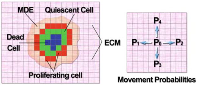
Schematic diagram (left) showing the key variables involved in the HDC model: tumour cells (colouration denoting cell state), extracellular matrix (ECM) and matrix degrading enzyme (MDE). Oxygen production comes from a pre-existing blood supply that is proportional to the ECM density. Diagram (right) shows the four possible directions each cell can move on the grid, driven by the movement probabilities P0 to P4, each cell can move at most one grid point at a time
With the HDC technique, we will use five coefficients P0 to P4 to generate the motion of an individual tumour cell. These five coefficients can be thought of as being proportional to the probabilities of a cell being stationary (P0) or moving west (P1), east (P2), south (P3) or north (P4) one grid point (Δx) at each time step (Δt) (see Fig. 1).
Each of the coefficient P1 to P4 consists of two main components,
Haptotaxis [30,48], migration up gradients of bound ECM molecules (f) generally dominates the movement rules and will bias movement towards higher ECM density. The motion of an individual cell is therefore governed by its interactions with the matrix macromolecules in its local environment. Of course the motion will also be modified by interactions with other tumour cells.
Tumour heterogeneity at the genetic level is well known and the so called “Guardian of the Genome”, the p53 gene is widely considered as a precursor to much wider genetic variation [49]. Loss of p53 function (e.g. through mutation) allows for the propagation of damaged DNA to daughter cells [49]. Once the p53 mutation occurs many more mutations can easily accrue, these changes in the tumour cell genotype ultimately express themselves as behavioural changes in cell phenotype. In order to capture the process of mutation we assign cells a small probability (Pmutat) of changing their phenotype during cell division. If such a change occurs the cell is assigned a new phenotype from a pool of 100 randomly predefined phenotypes within a biologically relevant range of cell specific traits.
At each time step a tumour cell will initially check if it can move subject to a cell–cell adhesion restriction, if it can, then the movement probabilities (above) are calculated and the cell is moved. A check is then made if the cell should become necrotic (see the following paragraph) or not. If it does not die, its age is increased and a check to see if it has reached the proliferation age is performed. If it has not reached this age then it starts the whole loop again. If proliferation age has been reached then a check is made to see if the criteria for proliferation are satisfied. If proliferation criteria are not met then the cell becomes quiescent. If they are satisfied then we check to see if this mitosis results in a mutation hit. All mutations occur in a random manner. This whole process is repeated at each time step of the simulation. For more detail see Appendix A.
Oxygen dynamics are important in the model as low levels of oxygen will cause necrosis, we will assume that if the oxygen level falls below a critical concentration (h) then the cell will die, the same is true for quiescent cells. Cells are also assumed to consume oxygen at a fixed rate (k) and quiescent cells will consume oxygen at a lower rate (kq). Cell proliferation and death create an evolving population (within the confines of the 100 randomly defined phenotypes) which we will use to examine both evolutionary and morphological changes that occur in a oxygen deprived environment.
3.2 Evolutionary hybrid cellular automata model
The basic structure of the Evolutionary Hybrid Cellular Automata (EHCA) model is a cellular automaton, which is coupled with a continuous field of oxygen (see Fig. 2). In order to capture the evolutionary dynamics of tumour growth each cell on the grid is equipped with a genotype, that dynamically determines cell behaviour and is inherited by the daughter cells under mutations. This allows the model to capture an important aspect of clonal evolution, i.e. a large number of different subclones that compete for space and resources [3,61].
Fig. 2.

Schematic layout of the EHCA model. The cells reside on a square lattice and each automaton element can either be occupied by a cancer cell or be empty. The cell type is indicated by the colour of the cell: proliferating cells are coloured red, quiescent green and dead cells are blue. Coupled together with the discrete lattice is a continuous field of oxygen supplied from the boundary
In real tumours some cells may acquire a selective advantage over other cells that can be viewed as a disruption in how the cells process information from their environment. In fact a cell can be viewed as a computing unit that given a certain environment “calculates” a phenotype or response, and this response depends on the genotype of the cell. For a normal cell the response to extended hypoxia is apoptosis, while a cancer cell with mutations in key genes (e.g. p53 [86]) would try to survive despite the low oxygen concentration. In the spirit of this each cell in the model is equipped with a decision mechanism that takes environmental variables as an input and from these determines the cellular behaviour as the output. This decision mechanism determines the update rules and implies that the state of an automaton element is not just characterised by if it holds a cancer cell or not, but by which cell it holds. The behaviour of the cells is determined by a response network, which is modeled using a feed-forward neural network [43]. These have traditionally been used for machine-learning tasks, but have been suggested as suitable models for signalling pathways [18]. The response network of the cells consists of a number of nodes that can take real number values. The nodes are organised into three layers: one input layer, that takes information from the environment, one hidden layer, and finally an output layer that determines the action of the cell. The response of the network determines if the cell will proliferate, become quiescent or go into apoptosis (see Fig. 2). The input to the network is the number of neighbours of the cell and the local oxygen concentration. In the initial genotype the competition for space determines if the cell will proliferate or become quiescent, while the oxygen concentration influences the apoptotic response. If the oxygen concentration falls below a certain threshold h the apoptosis node is activated and the cell dies. This implies that the behaviour of the cell is affected by the local oxygen concentration, but also changes it, as the response of the cell affects the oxygen consumption. Each time step of the simulation the oxygen concentration is solved and the cancer cells are updated and consume oxygen according to their network response. A proliferating cell consumes nutrient at a rate k, while a quiescent cell has a reduced consumption of kq < k and apoptotic cells do not consume any nutrients. This gives rise to a complex feedback between the cells and the oxygen concentration that will dictate the growth dynamics of the tumour.
The behaviour of the response network is determined by network parameters, which are copied from parent to daughter cell during cell division. This is done under mutations, which implies that the behaviour of the daughter cell might be different from its parent. When available space and oxygen are limited resources this will give rise to clonal evolution where only the fittest cells survive. A more detailed description of the model can be found in Appendix B.
3.3 Immersed boundary model of growing tumour
The immersed boundary model (IBCell model) of tumour fingering captures interactions between two-dimensional fully deformable cells and cell microenvironment that contains other neighbouring cells and a diffusive nutrient. The structure of each individual cell includes an elastic plasma membrane modelled as a network of linear springs that defines cell shape and encloses the viscous incompressible fluid representing the cytoplasm and providing cell mass. These individual cells can interact with other cells and with the environment via a set of discrete membrane receptors located on the cell boundary. In particular, every boundary point serves as a membrane receptor used to sense concentrations of nutrients distributed in the extracellular matrix. Moreover, each point can either be engaged in adhesion with one of the neighbouring cells (adhesive receptor), or can be used to determine sites of fluid transport during cell growth (free growth receptors). Cell growth is modelled by introducing couplets of fluid sources and sinks placed around the free growth receptors that collectively model transport of the fluid across the cell membrane. This results in expansion of the cell area until it is doubled. Then, additional boundary forces are used to create the contractile ring splitting the host cell into two daughter cells of approximately equal areas. Orientation of cell division is determined entirely by cell shape and the contracting springs are placed such that cell division is orthogonal to the cell longest axis. Cell–cell adhesion is modelled as forces acting between boundary points of two distinct cells if they are sufficiently close to one another. Figure 3a shows a small cluster of adherent cells with adhesive and growth receptors distributed along cell boundaries. Separate cells are connected by adhesive springs. Figure 3b shows morphological changes in a single proliferating cell.
Fig. 3.
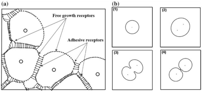
a A portion of a small cluster of adherent cells in the IBCell model. Cell boundary points (dots) are connected by short linear springs to form cell membranes (grey lines); cell nuclei (circles) are located inside cells and are surrounded by cell cytoplasm modelled as a viscous incompressible Newtonian fluid; separate cells are connected by adherent links (thin black lines); growing cells acquire the fluid from the extracellular space through the free membrane receptors. b Morphological alterations in a proliferating cell: 1 a cell ready to grow, 2 an enlarged growing cell with two daughter nuclei, 3 formation of the contractile ring orthogonal to the cell longest axis, 4 cellular division into two daughter cells of approximately equal areas
A general algorithm of the cell life cycle consists of three steps: (1) inspection of all cell membrane receptors to determine the total nutrient concentration sensed by the cell from the surrounding extracellular matrix, if this total nutrient concentration falls below the threshold value h the host cell is considered hypoxic; (2) nutrient uptake near each membrane receptor of all cells, viable and hypoxic (however, since nutrient uptake is modelled using the Michealis–Menten formulation, its uptake around the hypoxic cells is much lower than near the viable cells); this process together with nutrient diffusion results in the formation of a non-uniform nutrient gradient; (3) inspection of all membrane receptors in a non-hypoxic cell to determine whether or not cell growth is inhibited by contact with other cells, if at least 20% of cell membrane receptors are free from cell–cell adhesive contacts, the host cell is allowed to grow by acquiring the fluid from the extracellular matrix. If the cell is too crowded by other cells its phenotype changes to a quiescent state until the space becomes available or the cell becomes hypoxic due to the lack of nutrients in the cell microenviroment. A mathematical formulation of this model is presented in Appendix C in more detail.
4 Impact of cell metabolism on tumour morphology
In order to understand the key role that nutrients play in driving changes in tumour morphology we use each of the three models to investigate how changes in cell metabolic parameters influence the structure of the developing tumour. Specifically we explore the parameter space of oxygen consumption rate k versus the oxygen threshold level h at which cells become growth arrested (i.e. hypoxic/necrotic/apoptotic).
In each of the models discussed above the exploration of the two dimensional parameters space (k, h) was accomplished by selecting 4 values for each parameter, in a dynamically interesting range, and then simulating the growth of the tumour at these 4 × 4 = 16 points in parameter space. We chose to vary the parameters in the following manner: oxygen consumption rate k = {k0, 3k0, 5k0, 7k0} and the threshold value h = {h0, 2h0, 3h0, 4h0}. The base values k0 and h0 may depend on a specific cell line, but since we are interested here in qualitative results only, we use parameters for the oxygen and metabolism of the EMT6/Ro mouse mammary tumour cell line. The value of a base hypoxic threshold h0 has been chosen to represent a small percentage of oxygen concentration that the cell would sense if placed in an optimal oxygen concentration c0. In all models this complies with the lower levels of oxygen observed inside multicell spheroids [58] and in various types of tumours when compared to normal tissues from which the tumours arose, (a range of 9–30% has been reported in [19]). The upper limits for both parameters used in our simulations may be outside of the physiological range of oxygen-related metabolism in EMT6/Ro cells, but we want to analyse these extreme cases since they result in distinct tissue morphologies.
For each of the three models we run multiple simulations starting with the same initial cluster of tumour cells embedded in a homogenous field of oxygen of optimal concentration c0 and allow cells to interact with their microenvironment and execute their life cycle algorithm as discussed in the above sections. This leads to the development of different tumour morphologies including the emergence of tumour fingering. The results are summarised in the form of a graphical table and are discussed for each model separately in the next three sections.
4.1 HDC model results
In this section we use the HDC model, as discussed in Sect. 3.1, to simulate tumour growth for a range of different nutrient consumption rates (k) and threshold values (h). All simulations have initially uniform oxygen, ECM and MDE non-dimensional concentrations of c0 = 1, f0 = 1 and m0 = 0 and are initiated with 50 tumour cells in the centre of the domain each with a randomly assigned phenotype. After 200 time steps the tumour cell distributions for each parameter combination (k, h) were gathered to produce Fig. 4. Since the tumour population has the potential to mutate (via mitosis) to one of a hundred randomly defined phenotypes the constraint on consumption is only a lower bound and can vary from k to 4k.
Fig. 4.
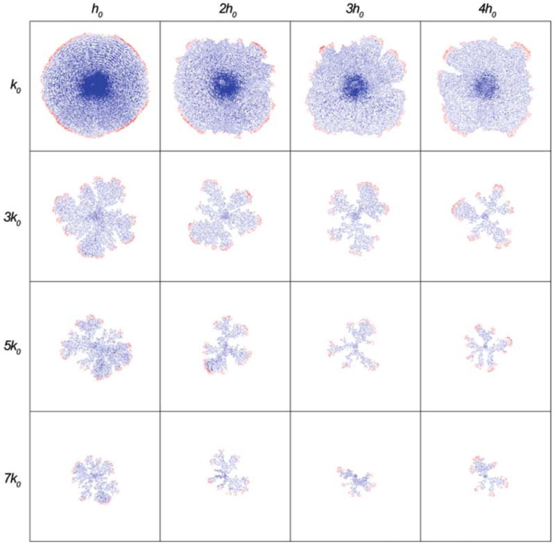
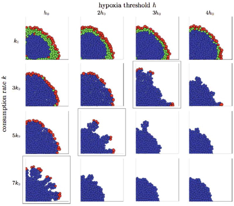
Tumour cell distributions at the end of 200 time steps for different combinations of the parameters (k, h) in the HDC model. Both parameters influence the morphology of the tumour: increasing k reduces size and produces fingering, increasing h has a similar but more subtle effect. Colouration represents cell type: red (proliferating); green (quiescent); blue (dead)
From Fig. 4, we see a diversity of tumour morphologies that share several common features. They consist of mainly dead (blue) and proliferating (red) cells which are mostly located on the outer rim of each tumour. We can clearly see the emergence of a fingering morphology as both the consumption rate and the threshold level are increased. Increasing the consumption rate also appears to decrease the overall size of the tumour in contrast to a more or less constant size as the threshold level is increased. Increasing the threshold level appears to cause the emerging fingers to take on thinner more elongated structures. If we examine the figures that run along the diagonal we see that the tumour becomes smaller and more fingered as we move from (k0, h0) to (7k0, 4h0) which is consistent with the above statements. These results clearly show that there is a direct correlation between the oxygen consumption rate and necrosis threshold value and tumour morphology.
One of the problems with showing the end result of the simulations is that the whole growth process that produced these results is missing. However, for all of the simulations in Fig. 4 the same growth process occurs and is of course dependent upon available oxygen levels. During the initial abundance of oxygen the tumour grows as a small round mass with smooth margins, further growth leads to more consumption of the available oxygen. In the HDC model oxygen is produced proportionally to the ECM density (under the assumption of a background vascular network, see Appendix A for further detail) and therefore as the tumour grows and degrades the ECM it is also destroying its own oxygen source. This results in necrosis and a dead central core forms within the tumour mass which is now surrounded by a thin rim of proliferating cells that continue to grow at the boundary of the tumour. When there is little consumption or the threshold level is low this rim of cells grows in a more or less symmetric manner but as these parameters are increased this symmetry is broken.
The time at which the necrotic core forms seems to be important as it is one of the first differences seen between the results collected in Fig. 4 (before the more obvious morphological changes occur). What we observe is that the earlier the appearance of the core the more likely fingering will occur—therefore the core in (k0, h0) forms much later than in (5k0, h0). The reason for this apparent relationship is mainly due to competition for available oxygen as a means of survival. As the nutrient consumption is increased and the threshold level increased the competition for the little available oxygen becomes dominant and one cell (or a small cluster of cells) will live at the expense of others by consuming the only oxygen that is left. Looking at the most fingered structures in Fig. 4 it is clear that none of them really have any large necrotic circular cores. Other differences relate to the evolutionary dynamics of the fingering versus the non-fingering tumour population, in particular the cells on the boundary that dominate the fingering population generally have more aggressive phenotypes, having low cell adhesion, high MDE production and migration abilities and lower oxygen consumption rates, but we will discuss this in more detail in Sect. 5.1.
4.2 EHCA model results
As detailed above we have varied the oxygen consumption rate k and the apoptotic threshold h. Because the model contains an evolutionary component the values of these parameters only determine the baseline or initial values. Mutations that occur in the population might alter the individual parameters of each cell, and h and k therefore only determine the initial values from which variation might occur. Each simulation was started with 4 ancestral cells at the centre of the grid. The oxygen concentration was initialised to a homogeneous concentration of c0 = 1 in the entire domain and the boundary condition was set to c(x, t) = 1, this is meant to imitate a situation where the tissue under consideration is surrounded by blood vessels that supply the tumour with oxygen via perfusion. Each simulation lasted 80 time steps (approx. 50 days) and at the end of each simulation the spatial distribution of cells was recorded.
The result of these simulations can be seen in Fig. 5, which shows the morphology for a range of oxygen consumption rates and apoptotis thresholds. From these simulations it is obvious that these parameters affect the morphology of the tumour. In all simulations the tumour starts growing with a proliferating rim and a core of quiescent cells, but when it reaches a certain size the diffusion of oxygen is not sufficient to supply the core of the tumour with oxygen. The time at which this occurs depends on both k and h and naturally occurs earlier in time for higher values of the two parameters. After the development of the necrotic core the tumour continues to grow, and at this stage the growth dynamics depend on the oxygen parameters. For low consumption rates and low apoptosis thresholds the tumour grows with a compact morphology with a smoothly growing leading edge that leaves a homogeneous distribution of dead cells in its wake, while for both higher consumption rates and apoptosis thresholds the proliferating rim instead breaks up and the tumour grows with a fingered morphology. What also can be seen is that varying the parameters leads to a gradual change in the morphology of the tumour. Increasing the consumption rate gives a smaller tumour with narrower fingers. An increasing apoptotic threshold also reduces the tumour mass, but seems to give rise to a qualitatively different change towards a fewer very narrow fingers.
Fig. 5.
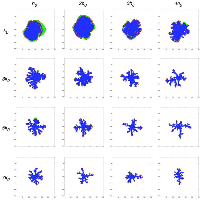
This plot shows the morphology in different regions of the parameter space (k, h) obtained using the EHCA model. Both parameters influence the morphology of the tumour and for high k and h we observe a fingered tumour morphology
The intuitive explanation for the fingering behaviour is that for high consumption rates there is not enough oxygen available to support the growth of all the cells on the boundary. This limited supply of oxygen results in competition between the cells at the boundary where only the fittest cells will survive long enough to go into cell division. When this occurs and the cell places its daughter cell outside the existing tumour boundary the daughter cells will consume oxygen and effectively creates a screen for access to oxygen for cells residing closer to the centre of the tumour. When the consumption rate is high compared to the oxygen concentration at the boundary of the tumour the cells have to rely on the flux of oxygen to survive long enough to go into mitosis. This implies that only the points on the boundary where the flux of oxygen is sufficient do we observe growth of the tumour. Similarly a higher apoptotic threshold also increases the competition as the cells will go into apoptosis at higher oxygen concentrations. The competition between cells at the boundary is amplified because it is easier to eliminate a neighbouring cell by screening it from oxygen and hence gaining a growth advantage. This increases the reliance on oxygen flux and destabilises the growth in a similar way.
4.3 Immersed boundary model results
In this model we varied the nutrient consumption rate k in the neighbourhood of a single cell receptor and the cell hypoxic threshold h, representing the limit of nutrient concentration sensed cumulatively through all cell membrane receptors, below which the cell behaviour changes from viable to hypoxic. In each presented case an identical cluster of viable cells (shown in Fig. 14a) was embedded into a homogeneous nutrient field of optimal concentration c0. All cells were allowed to execute the three-step cell life cycle described in Sect. 3.3 over the time corresponding to 11 average cell cycles and the results are summarised in Fig. 6.
Fig. 14.
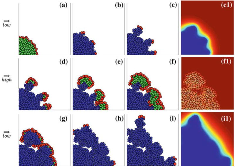
A three-stage scenario of tumour growth driven by a switching nutrient supply simulated using the IBCell model. Top row a–c tumour growth in the environment with low supply of nutrients, formation of finger-like cohorts of cells with cell growth restricted only to the tips is a result of cell competition for nutrients. Middle row d–f tumour growth in the environment with high supply of nutrients, tissue re-growth and expansion is an effect of lack of hypoxia, the emergence of a population of quiescent cells is due to cells competition for space only. Bottom row g–i tumour growth in the environment with low supply of nutrients—as in the top row, the formation of finger-like cohorts of cells with cell growth restricted only to the tips is due to cell competition for nutrients. The right column shows corresponding gradients of nutrients. An accompanying simulation movie is available as ESM
Fig. 6.
Final tumour configurations from the IBCell model obtained for various consumption rates and hypoxic thresholds, all presented at a time corresponding to 11 average cell cycles from pattern initiation. Three different patterns are observable: finger-like morphology (framed diagonal), continuous growth with smooth tumour boundaries (above the diagonal), and tumour growth suppression due to lack of nutrients (below the diagonal). Cells are colour-coded as follows: red growing; green quiescent; blue hypoxic
This figure shows three different morphologies of growing tumours: large clusters with smooth boundaries, medium size clusters with finger-like extensions and small clusters of non-growing cells. Only tumours shown in the top row contain quiescent cells (green) that emerge when the nutrient concentration in the cell vicinity is sufficient for the cells to remain viable but there is no space for the cell to grow. The presence of these quiescent cells is a result of low oxygen consumption. However, the number of layers of quiescent cells decreases with increased level of hypoxic threshold since higher values of h are more quickly achieved by the cells leading to early change in cell phenotype from viable to hypoxic (blue). In all other cases the quiescent cells appear sporadically and almost all cells are forced to enter the hypoxic state right after they are born. The first picture shows a couple of growing cells (red) inside the tumour cluster. However, those cells become quiescent before they double their area due to the development of new adhesive connections with their neighbours upon their enlargement.
There is a clear separation of tumour morphologies along the diagonal (framed pictures) with the exception of the first row. All tumours above the diagonal have compact, solid shapes with smooth boundaries that are an effect of constant cell growth in the proliferating rim expanding continuously over the cluster perimeter. In all presented cases the number of cells in the whole cluster has been doubled when compared with the initial number of cells. In contrast, all tumours below the diagonal show growth arrest, some of them in the very early stages of their development. The picture in the right corner shows a cluster which gained only 5% more cells than its initial configuration. This is an effect of cell growth arrest due to hypoxia levels that are rapidly achieved by viable cells, when the oxygen consumption rate is high. Some of these tumours show small non-growing extensions that suggest a potential for developing finger-like extensions in slightly modified conditions. An evident finger-like morphology appears in three cases on the diagonal (framed pictures). Here the rate of oxygen consumption is high enough to select a few leading cells that gain proliferative advantage over their neighbours by depleting the oxygen concentration in their vicinity leading subsequently to growth suppression of all cells around and behind the growing fingertips. In general, when one of the parameters is kept fixed and the second is increased the tumour morphology changes from solid compact large clusters of cells with smooth boundaries to medium size clusters of cells with finger-like extensions to small clusters of non-proliferating cells that may exhibit small sprouts of cells that remain in the growth arrest.
To investigate closer the mechanisms of formation of finger-like tissue extensions, let us inspect three configurations from Fig. 6 with significantly different parameters: (k0, h0) representing solid tumours, (7k0, 4h0) representing tumours with finger-like morphology, and (7k0, 4h0) representing tumours in growth arrest. In each case we examine the total concentration of nutrients sensed by each cell separately and the percentage of free growth receptors on each cell boundary. The results together with horizontal lines representing the hypoxic thresholds and vertical lines representing the growth threshold (20% of free growth receptors) are shown in Fig. 7. The first graph, Fig. 7a, confirms that the majority of cells with 20% or more of free growth receptors are actually growing (red), all quiescent cells (green) lie in the region above the hypoxic threshold and below the growth threshold, and almost all hypoxic cells (blue) are starving and are overcrowded. In contrast, Fig. 7b shows that numerous hypoxic cells lie above the growth threshold, that is they maintain more than 20% of their receptors free from cell–cell adhesion, so their growth suppression is due to low levels of oxygen in their vicinity and not to overcrowding, this suggests that the tissue fingers would not form if the cells were more resistant to starvation. This also leads to the conclusion that the finger-like morphology is rather a result of hypoxia-related growth suppression than overcrowding. Figure 7c shows in turn, that all cells in the growth arrested tumours lie well below their hypoxic threshold, that is they are exposed to nutrient concentrations much lower than the values at which cells switch their phenotypes from viable to hypoxic. This shows that decreasing the hypoxic threshold with the same consumption rate will still produce a growth arrested tumour. This is confirmed by the final tumour configurations in the last row of Fig. 6 where all tumours except the first on the left lack proliferating cells.
Fig. 7.
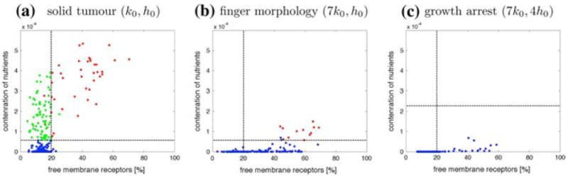
Distribution of all cells according to the concentration of nutrients sensed by each cell and the percentage of free growth receptors in a solid tumours, b tumours with finger-like morphology, c tumours in growth arrest from simulations in Fig. 6. Horizontal lines represent the hypoxic threshold. Vertical lines represent the 20% growth threshold. Cells are colour-coded as follows: red growing; green quiescent; blue hypoxic
5 Nutrient-dependent tumour morphology and evolution
It is clear from the previous results that nutrient starvation leads to a fingering morphology in all three models. The proliferating cells are located on the tumour fingertips, and thus exposed to higher concentrations of oxygen, grow at the expense of their closest neighbours causing starvation and growth arrest. This, in turn, amplifies the growth advantage of cells at the leading edge and further enhances the invasion of surrounding tissue. Whether cell starvation is a result of high cell metabolism or of limited oxygen supply (note that reducing the amount of available oxygen gives similar effects to increasing the consumption rate of the cells), it creates an environment dependent pressure for selection of the most aggressive cells capable of survival. Thus, since a harsh environment induces tumour fingering, whereas a mild environment gives rise to tumours with smooth margins, is it possible to reverse the fingering morphology by simply increasing the available oxygen levels and if so how will this effect the growth and evolutionary dynamics of the tumour population?
We address these questions by choosing one of the previously described cell lines (for each model separately) that gave rise to tissue fingering and then induce a change in the microenvironment by switching the external supply of oxygen between high and low concentrations. This imposes two different forms of competition upon the tumour cells, for space and nutrients in the poor oxygen microenvironment, and for space only in the oxygen rich microenvironment. In each phase, the tumour tissue is allowed to grow and develop producing different morphologies as well as different phenotypic and genotypic characteristics. To show that the tumour morphologies are typical for each phase, we use a double switch in concentration of supplied oxygen: high-low–high-low (similar to that used in [12]). The mechanism of oxygen switch is the same in all three models, but the duration of each switch phase may be different and depends on the model under consideration. In the EHCA Model all phases are equally timed, but the HDC Model requires the low oxygen phases to last longer because of cell migration effects. In the IBCell Model the switch in oxygen supply is executed after the cell pattern is clearly developed, and thus the phases of low or high oxygen supply are not timed equally.
In all three models we describe the morphological changes in the developing tissue as well as the population dynamics with regards to the subpopulations of growing, quiescent and dead cells. For the HDC and EHCA models we also discuss the evolutionary dynamics and argue that much of the evolutionary change is due to the extreme changes in the tumour microenvironment. For the IBCell Model we investigate how the dynamics of the growing tumour are driven by activity of the cell membrane receptors. The results of simulations of each model are presented in the next three sections.
5.1 HDC model results
To test the hypothesis that the fingering morphology can be reversed by manipulating the available oxygen levels we implemented the following scenario: we grew the tumour using the parameters (5k0, h0), see Fig. 4, initially in an oxygen rich environment (c = c0) until t = 60. We then dropped the oxygen concentration (c = 0.25c0) until t = 160 where it is set to high (c = c0) again and then finally for t = 220–320 we impose the low oxygen environment (c = 0.25c0). During the high oxygen phases, the tumour cells also consume oxygen but it is always replaced.
Growth dynamics
Figure 8 shows the simulation results with the tumour cell and oxygen concentrations at t = 60, 160, 220 and 320. After the first period of high oxygen the smooth circular tumour contains a mixed population of proliferating and quiescent cells and does not contain any necrotic cells. However, as soon as the oxygen level drops we immediately see the emergence of the fingering morphology and a circular necrotic core. The population is now dominated by necrosis with only a few proliferating cells, on the tips of the fingers, and no quiescent cells. Increasing the oxygen level again results in the fingers filling out and merging such that the boundary of the tumour becomes smooth again. We also see the remergence of the quiescent population. When the oxygen level is dropped for the final time we again see small fingers protruding from the smooth necrotic mass. The quiescent tumour population again becomes extinct and is dominated by necrotic and proliferating cells. The outcome is clear: under harsh conditions, when oxygen is in short supply, the morphology of the tumour is invasive (t = 160; t = 320). In mild conditions, the morphology is non-invasive (t = 60; t = 220).
Fig. 8.
Simulations results from the HDC model showing the tumour cell distributions at the end of each switch in oxygen concentration: a high (t = 60); b (i) low (t = 160); c high (t = 220); d (i) low (t = 320). Colouration represents cell type: red proliferating; green quiescent; blue dead. The oxygen concentration fields are also shown for both the low regimes: b (ii)t = 160 and d (ii)t = 320. An accompanying simulation movie is available as Electronic Supplementary Material (ESM)
These results also indicate a relationship between the invasive morphology and the quiescent tumour cell population. To investigate this we tracked the three tumour sub-populations (proliferating, quiescent and necrotic) over time and the results are shown in Fig. 9. From the figure it is clear that during the oxygen poor regimes there are almost no quiescent cells and in the oxygen rich regimes there are a large proportion of quiescent cells. To some extent this seems logical as within the nutrient rich environment all of the tumour population has the potential to proliferate and therefore space becomes a limiting constraint leading to the growth of the quiescent population. However, in the nutrient poor environment only the select few cells on the boundary of the tumour have the chance to proliferate and this is precisely where no space constraints exist. This may have some important implications for the treatment of real invasive tumours if valid, since a large percentage of chemotherapeutic drugs specifically target proliferating cells.
Fig. 9.
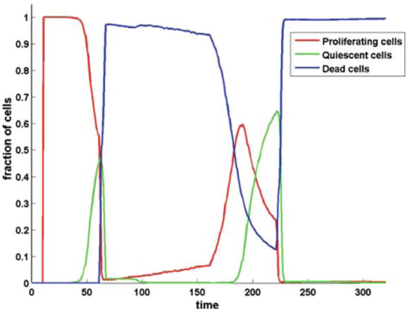
Time evolution of the tumour subpopulations for the oxygen switch simulation shown in Fig. 8: proliferating (red), quiescent (green) and dead (blue)
Evolutionary dynamics
An important benefit of using an individual based simulation approach is that at the same time as we simulate tumour growth we also track the numbers of the different phenotypes in the population. Figure 10 shows a plot of the relative abundance of each cell phenotype over the time of this simulation. During the first high oxygen period all of the phenotypes are more or less equally represented with no single dominant clone, however, as soon as the oxygen level is dropped we see the emergence of a single aggressive phenotype (shown with a thick purple line). This phenotype slowly grows to completely dominate the population in the low oxygen phase and as a result of this it also dominates the following high oxygen phase. It should be noted that other phenotypes are emerging during this second high oxygen phase, this can be seen from the fact that the purple line decreases, but their influence is small compared to the dominant clone. In the final low oxygen phase we see a sharp initial drop in the population due to the mass induced necrosis (also seen in the 1st low oxygen phase) of the low nutrient environment. This means there is only a small living population and therefore potentially only a few phenotypes can survive, however, it is the same aggressive phenotype that dominates again. An aggressive phenotype here is defined as one with a low proliferation age, high matrix degrading enzyme (MDE) production rate, zero cell–cell adhesion value and high haptotaxis coefficient.
Fig. 10.

Time evolution of the relative abundance of each of the 100 phenotypes for the oxygen switch simulation shown in Fig. 8. The most abundant phenotype is highlighted with a thicker line and the regions when the oxygen concentration is high are highlighted in grey
What is interesting from these results is the fact that the same aggressive phenotype (thick purple line in Fig. 10) dominates in the latter three phases (i.e. the low, high and low oxygen levels) and during the high oxygen phase no fingering is observed. The implication of these results is that an invasive outcome appears to be co-dependent upon the appropriate cell phenotype in combination with the right kind of microenvironment. In this case the phenotype is an aggressive one and the microenvironment is a harsh one. The cooperation, or more accurately the competition, that these two invasive properties confer upon the tumour population create a fingered invasive tumour. Potentially other combinations may lead to the same outcome (e.g. heterogeneous ECM, see [5]), however, within the nutrient dependent context of these simulations this is the only combination that results in invasion.
5.2 EHCA model results
For the EHCA model the switch in oxygen supply is equally timed and we allow the tumour to grow in a high oxygen concentration for 0 ≤ t < 30 then set the oxygen to its normal level for 30 ≤ t < 60, bring it back to high for 60 ≤ t < 90 and then finally set it to its normal level for 90 ≤ t ≤ 120. This gives rise to two distinct regimes in the growth: one where there is no competition for oxygen, and one where the cells have to compete for the limited supply of oxygen. Consequently we expect to observe two separate regimes in the evolutionary dynamics. Each simulation was started with an initial population of 100 cells and these cells each have a unique genotype which is one mutational step away from the ancestral genotype. The baseline nutrient parameters of all cells in the simulation were set to (k, h) = (5k0, h0), which corresponds to fingered growth in normal oxygen concentration (see Fig. 5).
Growth dynamics
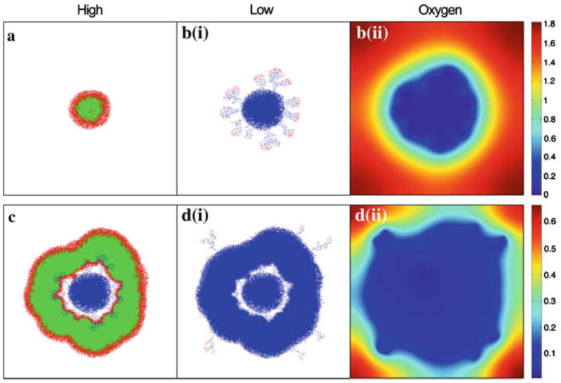
The results of this experiment can be seen in Fig. 11, which shows the spatial distribution of cells for t = 30, 60, 90 and 120, and oxygen concentration for t = 60 and 120. The tumour starts growing with a rim of proliferating cells and a core of quiescent cells, but because the supply of oxygen is unlimited we do not observe the development of a necrotic core. On the other hand when the oxygen supply becomes limited at t = 30 the tumour has grown larger than the critical size at which it develops a necrotic core. This leads to widespread cell death in the entire tumour and only a few isolated island of subclones which can survive in the low oxygen concentration remain. These clones start proliferating and develop a fingering morphology towards the boundary of the domain, which is the source of the nutrient. When the oxygen is shifted up again we observe a rapid re-population of the previously necrotic core and a return to the previous morphology. At the second round of nutrient starvation we observe dynamics similar to the first occurrence: massive cell death followed by a fingered morphology.
Fig. 11.
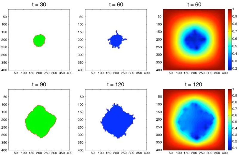
The spatial distribution of cells (left and middle columns) and oxygen concentration (right column) for the oxygen switching experiment using the EHCA model. In the high oxygen environment the tumour consists mostly of quiescent cells and grows with a round morphology, while in the low oxygen environment the tumour is dominated by dead cells and we observe a fingering morphology. An accompanying simulation movie is available as ESM
The dynamics can also be followed in Fig. 12, which shows the time evolution of different cell states (proliferating, quiescent, dead) in the tumour. At the beginning of the simulation (0 ≤ t < 30) we see a decrease in the fraction of proliferating cells, which is due to the fact that the area of the proliferating rim grows proportional to the radius R, while the number of quiescent cells grow at a rate R2 (proportional to the area). At t = 30 we observe a rapid increase of dead cells and a corresponding drop in quiescent cells. Now during the nutrient starved regime the proliferating cells outnumber the quiescent cells. This is due to the fingered morphology, where the cells reside on the tips of the fingers and the oxygen concentration drops so sharply that few cells can survive in a quiescent state. When the oxygen is returned to the high level (t = 60) the centre of the tumour is re-populated, which leads to a decrease in dead cells, which are being replaced by living cells. during the second phase of the oxygen poor regime (t = 90) we observe similar dynamics as the previous time.
Fig. 12.
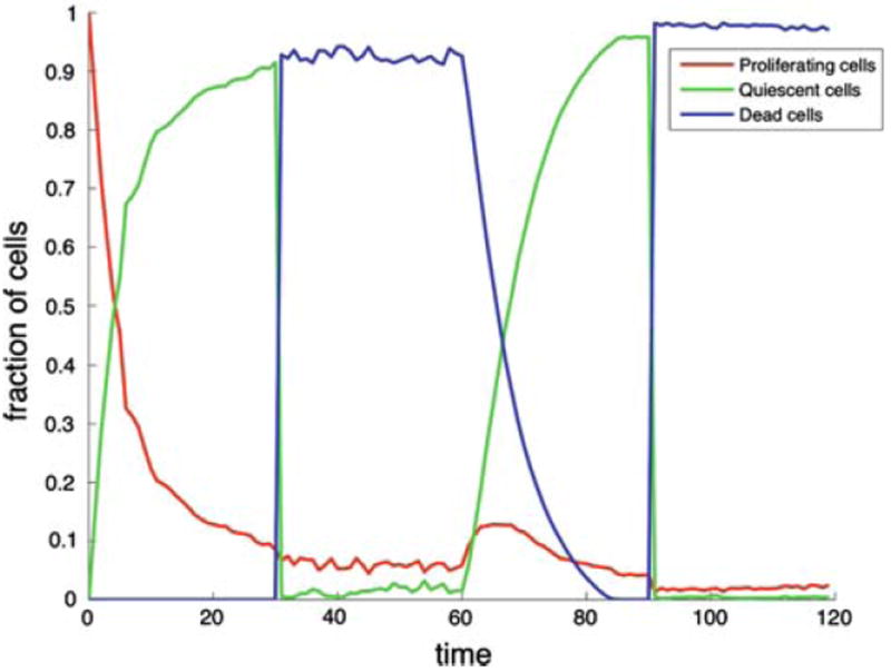
The time evolution of different cell states in the cancer cell population for the oxygen switching experiment shown in Fig. 11. The different growth regimes can clearly be distinguished, where quiescent cells dominate the high oxygen, while dead and proliferating cells are most abundant during the low oxygen
Evolutionary dynamics
The evolutionary dynamics were measured by looking at the time evolution of the phenotypes in the population. By phenotype we mean a set of cells that behave in the same way, but are not necessarily of the same genotype (i.e. have the same network parameters). The behaviour of a genotype can be quantified by measuring the fraction of the input space that each of the corresponding responses occupy. This gives us a 3-dimensional vector S = (P, Q, A), that we term the response vector, which reflects the behaviour of the cell. The initial cell has a response vector of S = (0.67, 0.18, 0.15), which means that 67% of the input space corresponds to proliferation, 18% to quiescence and 15% to apoptosis. We now identify two cells as being of the same phenotype if their response vectors agree. In order to keep the number of phenotypes at a manageable level and to simplify the analysis of the phenotypes each entry of the response vector was binned into 10 equal sized bins (i.e. 0, 0.1, 0.2, etc.). This reduces the number of unique phenotypes in the simulation from approximately 350 down to 50.
The dynamics were also measured on the genotype level by looking at the Shannon index [83], a measure of the genotypic diversity in the population. It is given by,
| (1) |
where pi is the probability of finding genotype i in the population and N is the number of distinct genotypes present in the population. Here we consider the cells to have the same genotype if their response networks are identical. The Shannon index reaches its maximum of 1 when all existing genotypes are equally probable (i.e for all i), and its minimum 0 when the population consists of only one genotype.
Figure 13a shows the time evolution of the phenotypes in the population, where the most dominant phenotypes have been highlighted and their response vectors have been included. In the initial oxygen rich environment we observe a co-existence of several phenotypes and smooth changes in the phenotype abundances. Some phenotypes clearly have a selective advantage and grow at the expense of other less successful phenotypes. Although most phenotypes exist in very small numbers we actually have 39 distinct phenotypes with non-zero abundance at t = 30 just before the oxygen is lowered to its normal level. At this point we see a radical change in the dynamics. Most striking is probably the fluctuations that the limited oxygen seems to induce. These are due to the fact that we now have a turn-over of cells due to cell death caused by the limited oxygen supply. After only a few time steps in the oxygen starved environment (t ≈ 33) the number of distinct phenotypes has dropped to 4, and we evidently have a stronger selection pressure in this growth regime. By the end of the oxygen starvation the phenotype that was dominant at t = 20 has gone extinct and the population is now dominated by a phenotype that emerged during the oxygen starved growth. During the following oxygen rich period the dynamics return to the previous smooth behaviour and we see little change in the abundance of the dominant phenotypes. The second round of oxygen starvation again leads to increased competition and the previously dominant phenotype increases even further and occupies approximately 90% of the population at the end of the simulation.
Fig. 13.

a The time evolution of the number of phenotypes for the oxygen switching experiment shown in Fig. 11. The most abundant phenotypes have been highlighted and their response vectors are displayed. b The time evolution of the genotypic diversity in the population. The two growth conditions clearly affect the diversity, where we observe a higher genotypic diversity in the low oxygen environment
This clearly shows that the evolutionary dynamics are different in the two growth regimes, and that they depend strongly on the oxygen supply. In the oxygen rich case the cells only have to compete for space, while when oxygen is limited the behaviour of the cells with respect to the oxygen concentration influences the fitness of a cell. This is reflected in the evolution of the response vector of the dominant phenotype. In the first oxygen rich period one of the dominant phenotypes has response vector S = (0.8, 0.1, 0.1), which means that it still has the capability to go into quiescence and apoptosis in some growth conditions. During the oxygen starved growth this phenotype declines and more aggressive phenotypes with smaller quiescence and apoptosis potential dominate. The second round of high oxygen again reflects the fact that space competition dominates this growth regime, but as soon as the oxygen is lowered the most aggressive phenotype S = (1, 0, 0) increases rapidly. This phenotype has completely lost the capability of remaining quiescent or going into apoptosis and can therefore be considered to be most aggressive phenotype possible. This suggests that competition for the limited oxygen creates a selection pressure towards more aggressive phenotypes with diminished quiescence and apoptosis potential that have a growth advantage in the poorly oxygenated environment.
If we now turn to the Shannon index in Fig. 13b we can see that this also is affected by the oxygen supply and exhibits distinct behaviour in the two growth regimes. Because the simulation is started with 100 different genotypes the Shannon index attains its maximal value of H(0) = 1. The diversity then decreases due to the growth of the tumour and the expansion of certain genotypes (see Fig. 13b). The reduction in Shannon index reflex the fact that the system evolves towards a situation where the tumour is dominated by a few genotypes. When the oxygen supply becomes limited we observe a sharp increase in the Shannon index. This implies that in the oxygen starved environment we have a more even genotype distribution where no dominant genotype exists. When the oxygen concentration is increased the diversity drops sharply and remains almost constant, but rapidly increases to the previous high value when oxygen becomes limited. From this we can conclude that the population in the oxygen starved environment can sustain a higher genetic diversity compared to the oxygen rich case and that this is due to the high selection pressure and cell turn-over that the low oxygen concentration induces.
These results are in sharp contrast to the phenotypic results and might even seem contradictory, but in order to explain this we must briefly discuss the difference between genotype and phenotype in the model. As mentioned before the genotype of a cell is determined from its network parameters, while the phenotype is determined from the outcome of the genotype or in other words the behaviour of the cell. This means that several genotypes can give rise to the same phenotype and this is the origin of the difference between the genotype and phenotype dynamics. The number of genotypes that existed in the simulation was approximately 600, while the number of clustered phenotypes only amounts to 50. Because selection only occurs at the phenotype level we can observe a high genotypic diversity in conjunction with a low phenotypic diversity. For example at t = 60 the Shannon index for the genotype distribution is H ≈ 0.9 while the corresponding measure for the phenotype distribution is H ≈ 0.3. The number of phenotypes naturally depends on how the phenotypes are binned, but the same analysis done with more bins showed similar dynamics (data not shown). We therefore appear to have a great deal of redundancy at the genotype level, i.e. the mapping from genotype to phenotype is not one-to-one, but many-to-one. This is also known to be true for real cells, where a single mutation in the genome does not necessarily give rise to a new phenotype.
5.3 Immersed boundary model results
We consider here the following three-stage scenario to determine the cell patterns arising in the low versus high nutrient concentrations. We initiate a simulation in the way described previously by embedding a cluster of viable cells into a uniform field of nutrient of optimal concentration and let the cells create a pattern as a consequence of their competition for nutrient. At this stage nutrient is only supplied once at the beginning of the simulation, it diffuses and is consumed by the cells. At the second stage we continuously supply nutrient of optimal concentration throughout the whole domain, such that all growing cells will be exposed to a nutrient concentration sufficient for their survival and will therefore only compete for space. At the third stage the nutrient supply will be cut off, thus again causing the viable cells to compete for nutrient and for free space.
Growth dynamics
We apply this three-stage scenario to a population of cells with a high nutrient consumption rate of 5k0 and a low hypoxic threshold of 2h0 from Sect. 4.3. The resulting patterns of growing tissue that arise in each growth stage are shown in Fig. 14. The right column shows nutrient concentrations in the whole computational domain corresponding to the neighbouring tumour snapshots. All other pictures show subpopulations of growing (red), quiescent (green) and hypoxic (blue) cells. Pictures in the top row show tumour growth in the low nutrient environment that takes place during the time corresponding to 11 average cell cycles. Initially the whole domain was filled with an optimal nutrient concentration for cell growth, but only cells in the outer rim can grow freely, whereas the inner cells are overcrowded and become quiescent, Fig. 14a. Initiation of finger-like sprouts with only a few growing cells located on the tips of fingers is a result of cell competition for nutrient. The growing cells are exposed to a higher nutrient concentration and proliferate continuously. The remaining cells are exposed to a low nutrient concentration, thus become hypoxic and non-responsive to proliferating factors, even if they have sufficient space for their growth, Fig. 14b. Further development of the finger-like tissue morphology is shown in Fig. 14c. Each tissue extension gains a few layers of cells, but cell growth is still restricted to the leading layer of cells. The steep gradient of nutrient shown in Fig. 14c1 confirms that growing cells take advantage of the higher nutrient concentration in their vicinity, whereas the remaining cells that are left behind are exposed to a depleted nutrient concentration. Results in the middle row show tumour growth after the change in nutrient supply, here, the nutrient is supplied at a constant rate in the whole computational domain over a time corresponding to 15 average cell cycles. We assume that the hypoxic cells are not allowed to re-enter into the growing phase, therefore the outgrowth of the tumour tissue shown in Fig. 14d–f arises only from a few cells that have previously been growing on the tips of tissue fingers. In this case, however, the nutrient is available in high concentrations, so there is no hypoxia of newly born cells, and cell growth is only restricted by the availability of space that gives rise to the subpopulation of quiescent cells. An increase in the number of growing cells is clearly observed compared with the previous stage, and daughter cells fill the space previously left behind by the fingers that results in a re-growth of a solid mass of tumour cells. Figure 14f1 shows that there is no gradient in nutrient concentration, lower concentration is only visible along cell membranes due to the nutrient uptake through the membrane receptors of all cells. Figures in the bottom row show tumour growth after the nutrient supply has been cut off again. This is similar to the situation shown in the upper row, and here again cells compete with one another for both nutrient and space. Due to nutrient uptake almost all quiescent cells become hypoxic and only cells in the outer layer are still growing (Fig. 14g). Emergence of new finger-like sprouts of cells is again due to cell competition for nutrient (Fig. 14h–i). Figure 14i1 shows pronounced nutrient gradients at the final stage of the simulation, corresponding to 14.5 average cell cycles.
The evolution of all three subpopulations of cells is shown in Fig. 15 starting from the initial time of the simulation that corresponds to 40 average cell cycles (the time needed to form an initial cluster) to the final time of 80 average cell cycles. All curves represent the percentage of cells in the whole tumour cluster. Three vertical lines indicate the times of change in nutrient supply, low denotes a one time supply, while high means constant nutrient supply; in both cases nutrients of optimal concentration are supplied in the whole computational domain. Since initially the cluster of cells is embedded into a homogeneous nutrient field of optimal concentration, no hypoxic cells are present, and cell classification into subpopulations of either quiescent or growing cells is based only on the amount of space available for their growth. However, due to high nutrient consumption the emergence of hypoxic cells is fast and they start to dominate the whole cluster after 2–3 average cell cycles, this is accompanied by extinction of the subpopulation of quiescent cells. Also the subpopulation of proliferating cells steadily diminishes reaching about 5% by the end of 11th cell cycle. After the change in nutrient supply from low to high, the percentage of growing and subsequently quiescent cells continuously increases reaching about 20% for growing and about 30% for quiescent cells after 15 cell cycles. The percentage of hypoxic cells decreases rapidly, however, their number is constant over this period, since the already hypoxic cells cannot re-enter into the growing phase and no new hypoxic cells emerge because the nutrient is available in high concentration. Upon the next switch to low nutrient supply, the subpopulation of growing cells decreases and all quiescent cells vanish after 2–3 cell cycles. The subpopulation of hypoxic cells again dominates the whole tumour cluster.
Fig. 15.
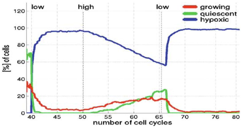
Evolution of subpopulations of growing (red), quiescent (green) and hypoxic (blue) cells over the time corresponding to about 40 cell cycles from the simulation shown in Fig. 14. Three vertical lines indicate times of change in the form of nutrients supply
Receptor driven dynamics
Since initiation and progression of all cell life processes in this model are directly related to the activity of cell boundary points, we analyse here differences between growing and hypoxic cells in the context of their response to cues sensed by individual cell membrane receptors, both nutrient and growth specific. Two pictures in Fig. 16 show the same configuration of tumour cells that has arisen after about 3 average cell life cycles in the simulation presented in Fig. 14. This cell configuration shows emergence of first hypoxic cells along the still smooth tumour boundary. The left picture shows a distribution of nutrient specific cell membrane receptors together with the magnitude of nutrient sensed by each receptor separately (vertical lines). The right picture shows the distribution of growth membrane receptors together with directions of expansion of all growing cells (arrows). Comparison of these two pictures confirms that the concentration of oxygen sensed by cell membrane receptors is higher at these boundary points that directly face the extracellular matrix and almost completely depleted at the points inside the tumour that are in contact with receptors of other cells. It is also clear from the left picture that hypoxic cells (blue) sense much smaller concentrations of oxygen than their growing neighbours (red). Note, however, that separate cells sense the same concentrations along common or near-by cell boundaries (vertical lines have the same length). From the right picture it is evident that growing cells expand mostly toward the space available in the extracellular matrix, and that cell–cell adhesive connections prevent cell growth. Two newly emerged hypoxic cells located on the boundary of the tumour cluster (indicated by triangles) still have access to a relatively high concentration of oxygen, but not high enough for cells to remain viable. The change in cell phenotype is a result of a direct competition for space between neighbouring cells. The nearby growing cells can expand faster due to their larger percentage of growth receptors, they also consume more oxygen leading subsequently to the depletion of nutrients in the vicinity of cells that grow slower and have been pushed behind the leading front. Once some cells gain such a growing advantage they expand faster forming the finger-like tissue extensions. In this model we assume that each membrane water channel used to transport the fluid into the growing cell has the same capacity, therefore the amount of the transported fluid and the speed of cell expansion are similar for each boundary growth receptor and do not depend on the nutrient concentration. In some sense the cells that dominate growth in the oxygen poor (fingering) regime are the most aggressive, i.e. they have less cell–cell adhesion and more growth receptors. This results in their faster growth and thus wider access to higher nutrient concentrations that are in turn used by the fast expanding cells leaving other cells in the vicinity depleted of nutrient that subsequently results in their growth suppression and hypoxia.
Fig. 16.
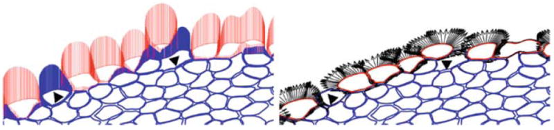
Distribution of cell boundary points used as nutrients-specific membrane receptors in the IBCell model, the magnitude of nutrients concentration sensed by each receptor is shown as vertical lines (left picture); and as growth-specific receptors to sense free space in cell vicinity, directions of cell expansion are shown as arrows (right picture). Hypoxic cells are shown in blue, growing cells in red, one dividing cell (red in the top right corner) is not expanding (right picture), but still senses high concentration of oxygen (left picture)
6 Theoretical discussion and conclusions
In this paper we have examined in detail the intimate relationship between the tumour nutrient microenvironment and the emergence of an invasive tumour morphology. In particular we considered the effects of changing metabolism parameters and nutrient availability. In both of these situations we observed tumour fingering, when metabolism was high or when nutrient availability was low. Intriguingly we were able to reproduce this behaviour over a range of parameters using three different models. Each of these models is single-cell-based and therefore allows us to vary specific cell parameters (such as cell metabolism, membrane receptors dynamics or genetic mutations) in each cell individually. All three models are also hybrid since they couple the discrete description of individual cells with a continuous description of the extracellular matrix and external factors, such as nutrient or enzyme concentrations. Moreover, all models can handle biological phenomena occurring over a range of spatial and temporal scales, such as membrane protein redistribution, cell life processes or genetic mutations. However, there are important differences between the models as each of them incorporates some biological phenomena not present in the others. Both the HDC and EHCA models consider cells as single lattice sites and IBCell represents cells as fluid filled elastic deformable membranes. Both the HDC and IBCell models include the effects of cell–cell adhesion, whereas EHCA does not, however it could be extended in this way. Both the EHCA and IBCell models are only proliferation driven whereas HDC is both proliferation and migration driven, and incorporates the effects of cell haptotaxis. All three models use oxygen as an external factor influencing cell responses, however the oxygen dynamics including production and consumption are different in all three models. Nevertheless, even with the differences in scale, technique and model assumptions we obtained strikingly similar results. The clear conclusion is that the invasive fingering morphology is not model or scale specific but emerges from the competition between cells for limited nutrients.
The morphologies obtained for high consumption rates are similar to those seen in diffusion limited growth processes like viscous fingering [29], electro-chemical deposition [56] and diffusion-limited aggregation DLA [91]. This is because the growth of the tumour under high consumption rates may be considered as similar to diffusion limited growth. In those processes the interface is advanced at a rate proportional to the gradient of a field u that satisfies Laplace equation ∇2u = 0 outside the structure with the boundary condition u = 0 at the interface. The assumption that the diffusion of oxygen is much faster than the cellular dynamics (e.g. proliferation) implies that the oxygen field is in a quasi-stationary state and thus satisfies ∇2c(x, t) ≈ 0. If we also assume a high consumption rate the oxygen field approximately satisfies c(x, t) = h at the tumour boundary. In this case growth is possible only where the tumour penetrates into the oxygen rich environment, i.e. the points where the flux |∇c(x, t)| of oxygen into the tumour is large. This only appears to occur at the tips of the fingers, where proliferating cells consume the nutrients. From this perspective the two growth processes are similar and not surprisingly they give rise to similar morphologies. When the oxygen consumption is reduced, the gradient of the oxygen fields become smoother and growth occurs more uniformly on the boundary. When the consumption is low the growth is almost completely uniform and corresponds to Eden like growth [34], where the probability of cell division is equal for all cells on the boundary. Changing the oxygen consumption rate (or the background oxygen level) thus corresponds to changing the growth probability distribution of the proliferating population on the boundary.
What also can be observed from the results is that the fingering only occurs when the proliferating rim contains only a few layers of cells. In fact it has been shown that for a simplified version of EHCA model (without the evolutionary component) the morphology of the tumour is determined by the width d of the proliferating rim [41]. When d is large the growth is stable and this results in a compact morphology, but when d decreases the growth becomes unstable leading to a fingered tumour morphology. For this simplified model the width d is given by
| (2) |
where τ is the cell proliferation age.
This shows that both the consumption rate k and the apoptotic threshold h affect d and it is therefore not surprising that increasing these parameters leads to branched growth. The width of the proliferating rim and its dependence on key model parameters has been considered previously from a purely continuous perspective [20-23].
However, what should be emphasised is the fact that the emergence of tumour fingering also went hand in hand with the selection of more aggressive phenotypes. The evolutionary dynamics produced several intriguing results and most of these were from the oxygen switch computations of Sect. 5. During the initial phase of these simulations whilst all cells are capable of proliferating only those on the outer boundary actually proliferate, due to the physical constraints of space availability. Even so the tumour population contains many phenotypes with varying degrees of aggressiveness. This all changes when the first low oxygen switch occurs, as this results in a large percentage of the population becoming growth arrested or being removed due to either hypoxia, necrosis or apoptosis. The remaining living cells are mainly dominated by a single aggressive phenotype which rapidly takes over and produces the fingering morphology typical of the low nutrient environment. As expected a smooth noninvasive morphology emerges during the second high oxygen switch. However, unexpectedly the noninvasive tumour population continues to be dominated by the same aggressive phenotype that produced the fingering morphology. In the final low oxygen phase, fingering reappears and again the same aggressive phenotype dominates. One important implication from these results is that tumour invasion, as represented by fingering, will only emerge if the right combination of tumour phenotypes and microenvironment occurs, i.e. context matters.
Another unexpected result is that the tumour cell genotypic diversity and the number of distinct phenotypes appear to be inversely correlated in the EHCA model. A unique property of this model is that it can distinguish between genotypes and phenotypes and simultaneously track them in the tumour population. In the oxygen poor microenvironment the number of tumour phenotypes rapidly drops whereas the genotypic diversity rapidly increases. The only explanation for this result is that several genotypes can give rise to the same phenotype. We therefore have a large degree of redundancy at the genotype level, i.e. the mapping from genotype to phenotype is not one-to-one, but many-to-one. This is also possible in real cells, where genomic mutations maybe silent and do not necessarily give rise to a new phenotype.
Many of these results revolve around the analogy that the switch from a non-invasive to an invasive tumour can be captured via a change in morphology, i.e. the emergence of finger like protrusions implies an invasive tumour. Figure 17 shows a section of a real invasive tumour boundary where the fingering morphology is clearly visible. Admittedly the fingers are somewhat less clearly defined in comparison to some of the simulations results in Sect. 4, but they do nonetheless capture the invasive leading edge as well as the difference in structure when compared to the noninvasive form (which would be a solid smooth mass). Whilst the relationship between fingering and invasion in real tumours remains to be formally defined, it is not uncommon to observe this phenomena in invasive tumours, however, other features, as yet unquantified, may also contribute to the invasive process.
Fig. 17.
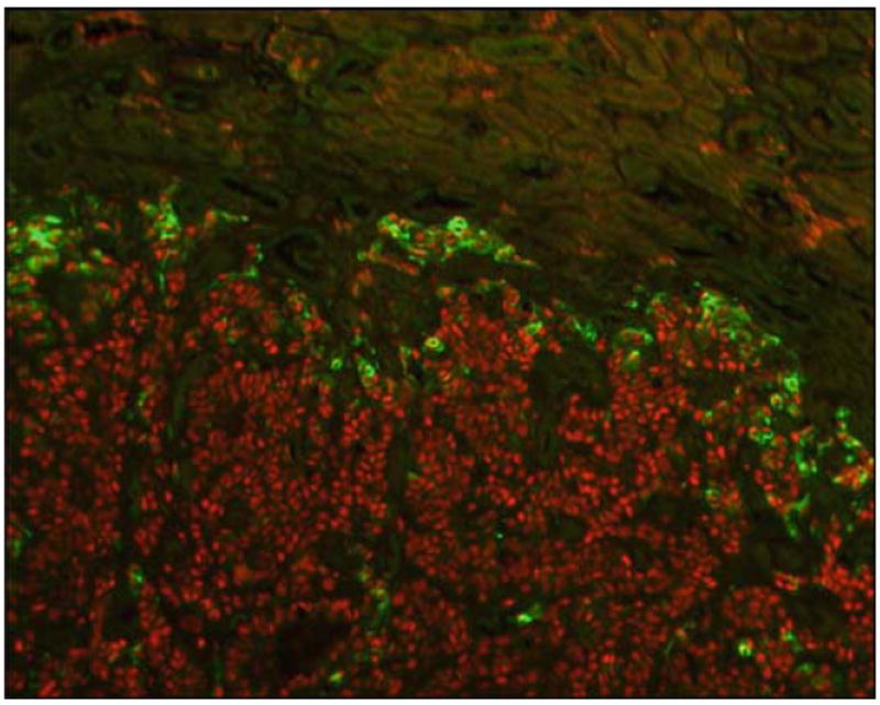
Tumour invasion of a mouse kidney showing tumour cells infiltrating between, and surrounding, kidney tubules. Cells are stained to show nuclei (red) and vimentin expression (green). Vimentin highlights cells undergoing the epithelial to mesenchymal transformation located specifically at the invading front and not in the tumour body. Adapted from Fig. 6 Ao et al. [13]
7 Biological implications
In a general sense, views on cancer invasion in the experimental biology community can be coarsely divided into cell-centric or gene-centric. In a cell-centric view, cancer cells become invasive because a particular state of differentiation, which happens to be infiltrative into surrounding tissue, is evoked by some external or internal factor, be it the microenvironment or some inappropriate developmental state. In this scenario, it appears as if, during cancer progression, some cells have somehow acquired the “invasive phenotype” (“malignant” cells). In a gene-centric view, particular combinations of gene activities, e.g., produced by accumulating mutations, translate into cells becoming invasive, whether or not this is in part due to some inappropriately evoked developmental program. These two views, polarised for the purpose of this discussion, are not really that different, though they lead to distinct experimental approaches to study invasion. Cell-centric view experimentalists will look for differentiating factors, gene-centric ones for molecular signatures of invading cells. They are not different, though, in the sense that they both consider invasion a property of the cancer cell, whether it is derived from a pre-assembled program inappropriately recalled (a developmental differentiated state), or an unfortunate molecular combination.
One major limit of both of these views is that they cannot explain why the outcome of malignant tumours is inescapably invasion. In this paper, we have brought forward arguments based on simulations that support a distinct view: invasion is an emergent property of the cancer progression process itself and not a property of the individual tumour cells. More specifically, the simulations of the 3 different models suggest that invasion is an outcome of microenvironment induced (or constrained) cancer cell population dynamics. In our case, dynamics were driven by differential proliferation induced by low nutrient conditions. It is not excluded, though, that other factors, such as matrix or proteases, may ignite population changes that inescapably lead to invasion.
To be clear, our simulations indicate that there is nothing intrinsically invasive about an invading cancer cell. While it requires certain properties in order to invade (e.g., proliferate, downregulate cell adhesion, or upregulate movement), these properties do not make a cell invasive. It is the competition between cells induced by a given microenvironment that produces a tumour cell population with invasive properties. This competition can only occur if there exists either variation within the cell population and/or variation within the microenvironment. It is important to note that variation within the cell population may be driven by several distinct (not necessarily mutually exclusive) mechanisms including, phenotypic variability (induced by genetic mutation, epigenetic gene regulation), phenotypic plasticity (natural capacity of a cell to modify its phenotypic traits) and noise inherent within cell biological systems. It can therefore be concluded that invasion is an emergent property of malignant tumours at the tissue scale and not the cell scale.
Supplementary Material
Acknowledgments
This work was supported by the U.S. National Cancer Institute Integrative Cancer Biology Program (U54 CA 113007).
Appendix A: Hybrid discrete-continuum model
We will base our mathematical model on generic solid tumour growth and focus on four key variables involved in tumour cell invasion, namely; tumour cell density (denoted by n), matrix degrading enzyme (MDE) concentration (denoted by m), ECM concentration (denoted by f) and oxygen concentration (denoted by c). The following system of coupled nonlinear partial differential equations describes the dynamics of the tumour cells, ECM, MDEs and oxygen,
| (3) |
where Dn, Dm and Dc are the tumour cell, MDE and oxygen diffusion coefficients, respectively, χ the haptotaxis coefficient and δ, μ, λ, β, k and α are positive constants. We should also note that cell–matrix adhesion is modelled here by the use of haptotaxis in the cell equation i.e. directed movement up gradients of ECM. Therefore χ maybe considered as relating to the strength of the cell–matrix adhesion. Since this model has already been published [5] we will not discuss its derivation here. We assume that the ECM, oxygen, tumour cells and consequently the MDEs, remain within the domain of tissue under consideration and therefore no-flux boundary conditions are imposed.
Discrete model
The HDC technique (see [4-8,10-12]) will be used to model the individual tumour cells and their interactions with one another and the continuum variables in the system (3). This first involves discretising (using standard finite-difference methods) the system of partial differential equations (3). We then use the resulting coefficients of the finite-difference stencil to generate the probabilities of movement of an individual cell in response to its microenvironment, further details can be found in [4]. As an illustration of the technique we only consider the tumour cell equation and discretise (3) in two spatial dimensions using central finite difference approximations to obtain the following,
| (4) |
where the subscripts specify the location on the lattice and the superscripts the time steps. That is x = i Δx, y = j Δx and t = q Δt where i, j, Δt, q and Δx are positive parameters.
The central assumption of the HDC technique is that the five coefficients P0 to P4 from (4) can be thought of as being proportional to the probabilities of a cell being stationary or moving to one it four orthogonal neighbours. The coefficient P0, which is proportional to the probability of no movement, has the form,
and the coefficients P1, P2, P3 and P4, which are proportional to the probabilities of moving west, east, south and north respectively, have the forms,
where the subscripts specify the location on the grid and the superscripts the time steps and i, j, Δt, q and Δx are positive parameters. From the above probabilities we see that if there were no ECM the values of P1 to P4 would be equal, with P0 smaller (or larger, depending on the precise values chosen for the space and time steps) i.e. there is no bias in any one direction and the tumour cell is less (more) likely to be stationary—approximating an unbiased random walk. However, if there are gradients in the ECM, haptotaxis contributes to the migration process and the coefficients P0 to P4 will become biased towards the direction of increased ECM concentration. The motion of an individual cell is therefore governed by its interactions with its local ECM environment but will also be modified by interactions with other tumour cells.
Individual-based processes
In addition to having the ability to move each cell has a collection traits that define its phenotype and describe how the cell will behave. The specific traits we consider are proliferation age, oxygen consumption, MDE production, haptotaxis coefficient and cell–cell adhesion. We have chosen these specific traits based on the current views of the invasive phenotype [42]. In the following paragraphs we discuss some of the key processes and traits involved in the HDC model of invasion (see [4] more detail discussion).
Cell–cell adhesion
To model cell–cell adhesion explicitly we assume each cell has its own internal adhesion value (Ai), i.e. the number of neighbours that it will preferentially adhere to. We therefore examine the number of external neighbours each cell has (Ae) and if Ae ≥ Ai then the cell is allowed to migrate, otherwise it remains stationary.
Death
For the tumour cell to survive it requires sufficient oxygen, since some tumour cells have been found to survive in very poorly oxygenated environments, we make the assumption that the concentration has to drop to h for cell death to occur. This assumption is also applied to quiescent tumour cells.
Proliferation
An individual cell will produce two daughter cells as a result of mitosis provided: (1) the parent cell has reached maturity (see mutation paragraph) and (2) there is sufficient space surrounding the parent cell for the two new daughter cells to occupy. In order to satisfy condition (2), we assumed that one daughter cell replaces the parent cell and the other daughter cell will move to any one of the parent cell’s four orthogonal neighbours that is empty. If no empty neighbours exist then the cell becomes quiescent and proliferation is delayed until space becomes available. Quiescent cells are assumed consume half the oxygen of normal cells.
Production/degradation
Since we are modelling individual tumour cells we must consider production and consumption of MDE and oxygen at the level of a single cell. In the continuum model Eq. (3) we have these rates as being proportional to the tumour cell density. Now these terms will only be active at a specific lattice point if a tumour cell is occupying that point (i.e. we take n = 1) otherwise they will be zero (i.e. we take n = 0).
Mutation
Here we shall consider 100 randomly defined phenotypes, each phenotype has an equal probability of being selected. A cells phenotype consists of a randomly selected, proliferation age (Phenage = 8 – 16 h), O2 consumption (PhenO2 = k – 4k), MDE production (Phenmde = μ – 4μ), haptotaxis coefficient (Phentaxis = χ – 4χ) and adhesion value (PhenA = 0 – 3). In most cases the range of values each parameter can take to define the phenotype were chosen to represent biologically realistic limits. Each cell is initially assigned the values of one of the hundred randomly selected phenotypes and for each subsequent proliferation there is a small probability (Pmutat) of further mutations occurring which will lead to another randomly selected phenotype and so on.
Simulation process for the hybrid discrete-continuum model
Each time step of the simulation process involves solving the discrete form of the system (3) numerically to generate the five coefficients P0 to P4. We then normalise these coefficients to obtain five corresponding final probabilities of motion, where normalisation simply means division by the total of the five coefficients. Probability ranges are then computed by summing the coefficients to produce 5 ranges, we then generate a random number between 0 and 1, and depending on the range which this number falls in, the current individual tumour cell under consideration will remain stationary or move to one of its orthogonal neighbours at each time step. This is provided the conditions imposed by cell–cell adhesion are satisfied. Once movement has occurred then the other individual based processes are considered and may result in cell death or proliferation and mutation.
Parameters
The time step in the simulation was set to Δt = 5 × 10⁻⁴ and the space step to Δx = 2.5 × 10⁻³ giving a grid size of (i, j) = (400, 400). The mutation probability is set to Pmutat = 0.01. The background oxygen concentration was set to c0 = 1.7 × 10⁻⁸ mol O2 cm−2 [5] and and the base oxygen consumption rate was taken to be k0 = 2.3 × 10⁻¹⁶ mol cell−1 s−1 [38]. The necrotic switch level h0 is assumed to be 5% of the initial oxygen concentration. For a complete list of parameters and how they were chosen see [5].
Appendix B: Evolutionary hybrid cellular automata model
The cell
Each cell on the grid is equipped with a decision mechanism, which determines the behaviour of the cell based on the cell genotype and the micro-environment in which it resides. The decision mechanism is modeled using an artificial feed-forward neural network [43]. The input to the network is the number of neighbours of the cell and the local oxygen concentration. The reason for this choice is that cancer cells often show weaker response to hypoxia-induced apoptosis [52] and that they tend to adhere less to their neighbours [25]. This implies that the input vector ξ will have two components, ξ = (n(x, t), c(x, t)). The phenotype of the cell is then determined by the output of the network. In our model the output nodes represent the response for proliferation, quiescence and apoptosis. As these three form a group of mutually exclusive behaviours (a cell cannot perform these responses simultaneously) the behaviour with the strongest response is chosen from these three, we call this the life-cycle response. If the proliferation node has the strongest response the cell divides and produces a daughter cell, if the quiescence node has the strongest response the cell remains dormant and if the apoptosis node is strongest then the cell dies via apoptosis. The network modulates the metabolism of the cell in two separate ways: Firstly the strength of the life-cycle response determines the overall energy consumption of the cell, secondly the oxygen consumption is lowered if the cell is quiescent. A graphical representation of the response network can be seen in Fig. 18. The output of the network is deterministic and depends only on the environmental input and the network parameters. These define the strength of connections between the different nodes and are represented as two matrices w, W and two threshold vectors θ and ϕ. When the cells divide the network parameters are copied to the daughter cell under mutations. The number of mutations that occur in the daughter cell network parameters is chosen from a Poisson distribution with parameter p. These mutations are then randomly distributed over the matrices and the incorrect copying is modeled by adding a normal distributed number s ∈ N(0, σ) to the daughter cell matrix or threshold entry, which means that x → x + s, for those entries x that are chosen for mutation. Mutations alter the connection strength between the nodes, which in turn changes how the cells responds to the micro-environment. If for example a mutation occurs in a connection that links the oxygen concentration with the apoptosis node this changes how the cell responds to the local oxygen concentration.
Fig. 18.
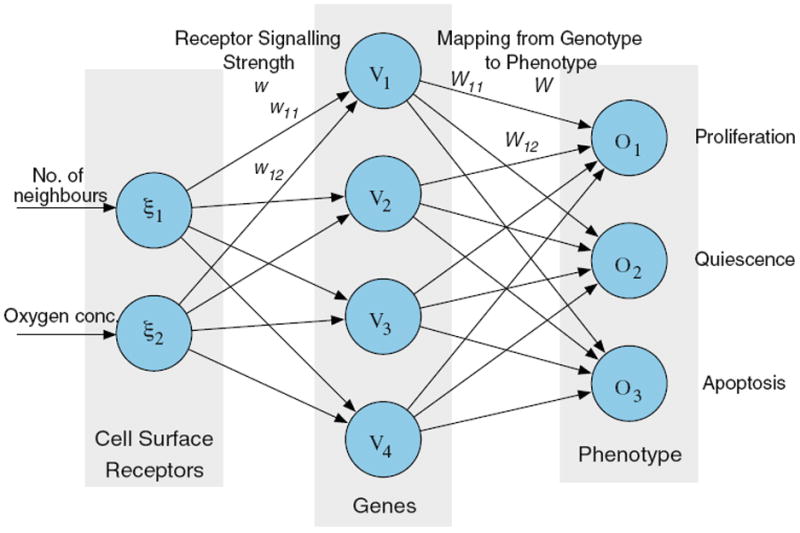
The layout of the response network in the cells in the EHCA model: the connections between the input layer and the hidden layer are determined by the connection matrix w and the connections between the hidden layer and the output layer are determined by W
Oxygen field
We only consider an oxygen field in the model and focus on how the oxygen impacts upon the growth and evolutionary dynamics of the model. A further simplification is that we neglect the decay of the oxygen and that we include the production of oxygen at the domain boundary by applying Dirichlet boundary conditions with constant functions. These boundary conditions are meant to imitate a situation were the tissue is surrounded by blood vessels, with constant nutrient concentrations, that supply the tumour with oxygen. This gives the equation that describes the oxygen field a simple form, similar to those in the models of [65] and [35]. The time evolution of the oxygen field (5) is governed by the following partial differential equation,
| (5) |
where Dc is the diffusion constant of oxygen and fc (x, t) gives the individual cell oxygen consumption rate for the cell at position x at time t. The oxygen field is solved on a grid of the same step size as the cells using an ADI-scheme [72]. This choice of space step implies that the consumption term in (5) is determined by each individual cell, and fc (x, t) is thus defined in the following way,
| (6) |
where k0 is the base consumption rate and F(x) is the modulated energy consumption of the individual cell occupying the automaton element at x.
Cellular automaton
The two-dimensional tissue under consideration is represented by a N × N grid. Each grid point can either be occupied by a cancer cell or be empty and also holds the local concentration of oxygen. The grid is characterised by a grid constant d, which determines the size of the cells. The grid points are identified by a coordinate x = Δx (i, j) i, j = 0, 1, …, N − 1. The chemical concentrations interact with the cells according to cellular consumption rates and are given appropriate initial and boundary conditions. Each time step the chemical concentrations are solved using the discretised equations and the tumour cells are updated in a random order. Every time step each cell is updated as follows:
The input vector ξ is sampled from the local environment (i.e the grid point where the cell resides).
A response R = R(ξ, G) is calculated from the network, where G represents the genotype of the cell, i.e. the network parameters.
The cell consumes oxygen according to its behaviour. If there is not sufficient oxygen present the cell dies from necrosis.
-
The life-cycle action determined by the network is carried out:
If proliferation (P) is chosen, check if the cell has reached proliferation age and if there is space for a daughter cell. If both are true the cell divides and the daughter cell is placed in a neighbouring grid point, if not the cell does nothing.
If quiescence (Q) is chosen the cell becomes quiescent.
If apoptosis (A) is chosen the cell dies.
If a cell dies from either apoptosis or necrosis it is no longer updated. Although the two death processes occur in different ways we will for simplicity treat them equally and consider the grid point where the cell resided empty in the next time step.
Parameters
The initial network, which is used as a “seed” in every simulation, is chosen so that the behaviour of the cell resembles that of an initial cancer cell phenotype. The response of the network therefore has to capture the essential behaviour of real cancer cells. The important features that we want to capture are: (1) cells should perform apoptosis if the oxygen concentration c(x, t) falls below a certain threshold h; (2) cells should not divide if there is no space for the daughter cell (contact inhibition), i.e. if n(x, t) > 3. The value of h is difficult to estimate as it depends on the cell type under consideration, but measurement performed in several types of tumours reveal that the oxygen concentration in the necrotic centre of the tumour is 0.5–30% of the concentration in the surrounding tissue [19]. We therefore estimate h0 to be 10% of the initial oxygen concentration. A network that satisfies the above specifications was constructed and was used as a starting point in every simulation. The background oxygen concentration was set to c0 = 1.7 × 10⁻⁸ mol O2 cm−2 [5] and and the base oxygen consumption rate was taken to be k0 = 2.3 × 10⁻¹⁶ mol cell−1 s−1 [38].
The grid size was set to N = 300, which means that we can simulate a tumour of radius 150 cells, which if we assume radial symmetry in a three-dimensional setting would correspond to a tumour consisting of approximately 1503 or 3 million cells. The time step in the simulation was set to Δt = 10−1 and the space step to d = 0.0025. The mutation probability is set to p = 0.01 [5] and the mutation strength to σ = 0.25. For the full list of parameters and an in-depth description of the model please consider [40].
Appendix C: Immersed boundary model
This model is based on the immersed boundary method and couples the mechanics of elastic cells, the viscous incompressible fluid in which the cells sit and the kinetics of nutrients distributed in the whole domain. Fluid flow is influenced by sources and sinks used to model transport of fluid across the cell membranes, as well as forces generated by the deforming elastic cell boundaries, while at the same time all elastic bodies move at the local fluid velocity. The nutrients are degraded in the local neighbourhood of all cells, and the cell behaviour depends on the total concentration of nutrients sensed by the host cell from the surrounding extracellular matrix. The immersed boundary method was introduced by Peskin to model blood flow around heart valves [69,70], and then it was successfully applied to many different problems involving fluid-structure interactions; compare [71, Sect. 9]. The immersed boundary model of growing cells has been used previously to investigate folding of the trophoblast tissue [81], development of early avascular tumours [76], emergence of tumour microregions [75], formation of different patterns of ductal carcinoma in situ [80], and cell self-arrangement into an epithelial acinus [78,79].
Governing equations
Since we are interested here in mechanisms that lead to the formation of invasive sprouts of cells from a solid mass of tumour tissue, it is sufficient to carry on all simulations in one quarter of a typical growth domain only, and to initiate all simulations from a predefined circular configuration of viable cells. This effective simulation domain is embedded into a slightly larger computational domain where the fluid and nutrient equations are solved. The nutrient is distributed in the whole computational domain—outside and inside the cells, however, its uptake takes place only in a local environment around cell membrane receptors, and these local values are also used to determine the total nutrient concentration sensed by the cell. This significantly reduces computational cost of all simulations, but still allows us to focus on the mechanisms of cell growth and cell competition for nutrients. An extension of this model to the whole domain is, however, straightforward (compare [75-77]).
The model is defined on a two-dimensional domain Ω with fixed Cartesian grid x = (x1, x2) that is common for the fluid and nutrient variables. The elastic membranes of all cells form a collection Γ = {Γi} of closed curves Γi defined in the curvilinear coordinates Xi (l, t), where l is a position along the boundary of the ith cell. The fluid inside and outside the cells is modelled as a homogeneous continuum with the same constant density ρ and viscosity μ. We assume that the fluid motion is governed by the Navier–Stokes equations (Eq. 7), where p(x, t) is the fluid pressure, u(x, t) is the fluid velocity, the external force density f(x, t) is defined at the boundaries of all cells (Eq. 9), and the source-sink distribution s(x, t) is taken around all growing cells (Eq. 10). The continuity equation with a source term (Eq. 8), describes the law of mass balance, where the source distribution s(x, t) is identically equal to zero on the whole fluid domain except at the point sources and sinks that are used to model cell growth. Conservation of mass must be preserved globally in the fluid domain Ω at each time t; that is, ∫Ω s dx = ρ ∫Ω (∇ · u) dx = 0.
| (7) |
| (8) |
| (9) |
| (10) |
| (11) |
| (12) |
| (13) |
Interactions between the fluid and the material points of all immersed bodies are defined in Eqs. (9)-(12). Here, the boundary forces Fi (l, t) in the ith cell Xi (l, t) represent the sum of different contractive-repulsive forces arising from elasticity of the cell plasma membrane, division of the host cell into two daughter cells and from interactions between distinct cells. Each of them satisfies Hooke’s law with a constant resting length Lα and a constant spring stiffness Fα, where α denotes one of the acting forces. These forces are applied directly to the fluid in a δ-layer region around the boundary Γi of the ith cell (Eq. 9), where δ is a two-dimensional Dirac delta function: δ(x) = δ(x1)δ(x2).
The fluid sources and sinks are distributed at the discrete collections of points (whrer p = + or p = −, respectively), located along the cell boundary Γi within the cell local microenvironment ΘΓi, that is . They are used to model transport of the fluid through the membrane of a growing cell in such a way, that fluid introduced in the sources inside the cell is balanced by the loss of fluid in the sinks outside the cell membrane for each growing cell separately. These source and sink contributions are then transmitted to the surrounding fluid using the Dirac delta function (Eq. 10).
In this model, the growth and survival of each cell depend on the concentration of nutrients c in the cell vicinity. Therefore, the activation of fluid sources in the ith cell takes place when the total concentration of nutrients at all boundary points of that cell exceeds the prescribed threshold value h. The value of c at the material point Xi (l, t) is equal to its local concentration around that point (Eq. 11). The strength of each balancing fluid sink is determined for each host cell separately to balance the total source distribution in that cell (Eq. 10).
The no-slip condition of a viscous fluid implies that the material points on cell boundaries are carried along with the fluid (Eq. 12).
The kinetics of c includes a constant source of value c0 continuously applied at the domain boundaries, uniform diffusion of c in the whole computational domain (with the diffusion coefficient D), and its degradation defined using the Michaelis–Menten formulation (with constants k and κ) that takes place within the local microenvironment of all cells ΘΓ=∪i ΘΓi. It is also assumed that initially the whole computational domain Ω is filled uniformly with an optimal concentration c0 (Eq. 13).
Model implementation
The model has been implemented using finite difference schemes for fluid and nutrient equations discretised on a common regular grid. The Navier–Stokes equations have been solved using the fast Fourier algorithm. Interactions between the fluid-nutrient grid and the material points of immersed bodies have been implemented using a bell-shaped discrete approximation to the Dirac delta function of bounded (16 points) support. The general algorithm includes: (1) determine growing cells by inspecting the total concentration of nutrients in their microenvironments; update the level of nutrients concentration by computing rates of its diffusion and consumption by individual cells; (2) calculate the total force density from the configuration of cell boundaries; spread those values to the neighbouring grid points to determine the forces acting on the fluid; (3) determine the source-sink distribution at points located along the boundaries of all growing cells; spread these values to the neighbouring grid points to find the local expansion rate on the fluid; (4) solve the Navier–Stokes equations for the fluid velocity field. (5) interpolate the fluid velocity field to each immersed boundary point and compute their new positions by moving them at the local fluid velocity using a forward Euler scheme. More details about this numerical implementation and physical parameters can be found in [81,75-77].
Parameters
Initially all cells are embedded into a homogeneous field of oxygen of optimal concentration c0 = 0.28 mM as reported in [24]. The base consumption rate is taken to be k0 = 1.475 × 10⁻⁸ moles/cm3 · s that is in agreement with the range of values 1–3 ×10⁻⁸ moles per cm3 of viable spheroid volume per second reported in [37]. The value of a base hypoxic threshold h0 has been chosen to represent 9% of oxygen concentration that the cell would sense if placed in an optimal oxygen concentration c0. The choice of all other parameters is discussed in detail in [75,78].
Footnotes
Electronic supplementary material The online version of this article (doi:10.1007/s00285-008-0210-2) contains supplementary material, which is available to authorized users.
Contributor Information
Alexander R. A. Anderson, Division of Mathematics, University of Dundee, Dundee DD1 4HN, Scotland, UK
Katarzyna A. Rejniak, Division of Mathematics, University of Dundee, Dundee DD1 4HN, Scotland, UK
Philip Gerlee, Division of Mathematics, University of Dundee, Dundee DD1 4HN, Scotland, UK.
Vito Quaranta, Department of Cancer Biology, Vanderbilt University School of Medicine, Nashville, TN 37235, USA.
References
- 1.Alarcon T, Byrne HM, Maini PK. A multiple scale model for tumor growth. Multiscale Model Simul. 2005;3:440–475. [Google Scholar]
- 2.Albini A, Sporn MB. The tumour microenvironment as a target for chemoprevention. Nat Rev Cancer. 2007;7:139–147. doi: 10.1038/nrc2067. [DOI] [PubMed] [Google Scholar]
- 3.Alexandrova R. Tumour heterogeneity. Exp Pathol Parasitol. 2001;4:57–67. [Google Scholar]
- 4.Anderson ARA. A hybrid discrete-continuum technique for individual based migration models. In: Alt W, Chaplain M, Griebel M, Lenz J, editors. Polymer and cell dynamics. Birkhauser; Basel: 2003. [Google Scholar]
- 5.Anderson ARA. A hybrid mathematical model of solid tumour invasion: the importance of cell adhesion. IMA J Math Med Biol. 2005;22:163–186. doi: 10.1093/imammb/dqi005. [DOI] [PubMed] [Google Scholar]
- 6.Anderson ARA. A hybrid multiscale model of tumour invasion: evolution and the microenvironment. In: Anderson ARA, Chaplain MAJ, Rejniak KA, editors. Single-cell-based models in biology and medicine. Birkhauser; Basel: 2007. [Google Scholar]
- 7.Anderson ARA, Chaplain MAJ. Continuous and discrete mathematical models of tumour-induced angiogenesis angiogenesis. Bull Math Biol. 1998;60:857–899. doi: 10.1006/bulm.1998.0042. [DOI] [PubMed] [Google Scholar]
- 8.Anderson ARA, Chaplain MAJ, Newman EL, Steele RJC, Thompson AM. Mathematical modelling of tumour invasion and metastasis. J Theor Med. 2000;2:129–154. [Google Scholar]
- 9.Anderson ARA, Chaplain MAJ, Rejniak KA. Single-cell-based models in biology and medicine. Birkhauser; Basel: 2007. [Google Scholar]
- 10.Anderson ARA, Pitcairn A. Application of the hybrid discrete-continuum technique. In: Alt W, Chaplain M, Griebel M, Lenz J, editors. Polymer and cell dynamics. Birkhauser; Basel: 2003. [Google Scholar]
- 11.Anderson ARA, Sleeman BD, Young IM, Griffiths BS. Nematode movement along a chemical gradient in a structurally heterogeneous environment. II. Theory. Fundam Appl Nematol. 1997;20:165–172. [Google Scholar]
- 12.Anderson ARA, Weaver AM, Cummings PT, Quaranta V. Tumor morphology and phenotypic evolution driven by selective pressure from the microenvironment. Cell. 2006;127:905–915. doi: 10.1016/j.cell.2006.09.042. [DOI] [PubMed] [Google Scholar]
- 13.Ao M, Williams K, Bhowmick NA, Hayward SW. Transforming growth factor-β promotes invasion in tumorigenic but not in nontumorigenic human prostatic epithelial cells. Cancer Res. 2006;66:8007–8016. doi: 10.1158/0008-5472.CAN-05-4451. [DOI] [PMC free article] [PubMed] [Google Scholar]
- 14.Araujo RP, McElwain DLS. A history of the study of solid tumour growth: the contribution of mathematical modeling. Bull Math Biol. 2004;66:1039–1091. doi: 10.1016/j.bulm.2003.11.002. [DOI] [PubMed] [Google Scholar]
- 15.Ben-Jacob E, Cohen I, Levine H. Cooperative self-organization of microorganisms. Adv Phys. 2000;49:395–554. [Google Scholar]
- 16.Ben-Jacob E, Garik P. The formation of patterns in non-equilibrium growth. Nature. 1990;343:523–530. [Google Scholar]
- 17.Bierie B, Moses HL. Tumour microenvironment: TGF, the molecular Jekyll and Hyde of cancer. Nat Rev Cancer. 2006;6:506–520. doi: 10.1038/nrc1926. [DOI] [PubMed] [Google Scholar]
- 18.Bray D. Intracellular signalling as a parallel distributed process. J Theor Biol. 1990;143:215–231. doi: 10.1016/s0022-5193(05)80268-1. [DOI] [PubMed] [Google Scholar]
- 19.Brown JM, Wilson WR. Exploring tumour hypoxia in cancer treatment. Nat Rev Cancer. 2004;4:437–447. doi: 10.1038/nrc1367. [DOI] [PubMed] [Google Scholar]
- 20.Byrne HM, Chaplain MAJ. Growth of non-necrotic tumours in the presence and absence of inhibitors. Math Biosci. 1995;130:151–181. doi: 10.1016/0025-5564(94)00117-3. [DOI] [PubMed] [Google Scholar]
- 21.Byrne HM, Chaplain MAJ. Growth of necrotic tumours in the presence and absence of inhibitors. Math Biosci. 1996;135:187–216. doi: 10.1016/0025-5564(96)00023-5. [DOI] [PubMed] [Google Scholar]
- 22.Byrne HM, Chaplain MAJ. Modelling the role of cell–cell adhesion in the growth and development of carcinomas. Math Comput Model. 1996;24:1–17. [Google Scholar]
- 23.Byrne HM, Chaplain MAJ. Free boundary problems arising in models of tumour growth and development. EJAM. 1998;8:639–658. [Google Scholar]
- 24.Casciari JJ, Sotirchos SV, Sutherland RM. Variations in tumor cell growth rates and metabolism with oxygen concentration, glucose concentration, and extracellular pH. J Cell Physiol. 1992;151:386–394. doi: 10.1002/jcp.1041510220. [DOI] [PubMed] [Google Scholar]
- 25.Cavallaro U, Christofori G. Cell adhesion and signaling by cadherins and ig-cams in cancer. Nat Cancer Rev. 2004;4:118–132. doi: 10.1038/nrc1276. [DOI] [PubMed] [Google Scholar]
- 26.Chaplain MAJ, Lolas G. Mathematical modelling of cancer cell invasion of tissue: the role of the urokinase plasmino- gen activation system. M3AS. 2005;15:1685–1734. [Google Scholar]
- 27.Chaplain MAJ, Graziano L, Preziosi L. Mathematical modelling of the loss of tissue compression resposiveness and its role in solid tumour development. Math Med Biol. 2006;23:197–229. doi: 10.1093/imammb/dql009. [DOI] [PubMed] [Google Scholar]
- 28.Cristini V, Frieboes HB, Gatenby R, Caserta S, Ferrari M, Sinek J. Morphologic instability and cancer invasion. Clin Cancer Res. 2005;11:6772–6779. doi: 10.1158/1078-0432.CCR-05-0852. [DOI] [PubMed] [Google Scholar]
- 29.Daccord G, Nittmann J, Stanley HE. Radial viscous fingers and diffusion-limited aggregation: fractal dimension and growth sites. Phys Rev Lett. 1986;56(4):336–339. doi: 10.1103/PhysRevLett.56.336. [DOI] [PubMed] [Google Scholar]
- 30.Debruyne PR, Bruyneel EA, Karaguni I-M. Bile acids stimulate invasion and haptotaxis in human corectal cancer cells through activation of multiple oncogneic signalling pathways. Oncogene. 2002;21:6740–6750. doi: 10.1038/sj.onc.1205729. [DOI] [PubMed] [Google Scholar]
- 31.Dormann S, Deutsch A. Modeling of self-organzied avascular tumor growth with a hybrid cellular automaton. In Silico Biol. 2002;2:393–406. [PubMed] [Google Scholar]
- 32.Drasdo D, Höhme S. A single-cell-based model of tumor growth in vitro: monolayers and spheroids. Phys Biol. 2005;2:133–147. doi: 10.1088/1478-3975/2/3/001. [DOI] [PubMed] [Google Scholar]
- 33.Düchting W. Tumor growth simulation. Comput Graphics. 1990;14:505–508. [Google Scholar]
- 34.Eden M. A two dimensional growth process. Proc 4th Berkpley Symp Math Stat Prob. 1961;4:223. [Google Scholar]
- 35.Ferreira SC, Martins ML, Vilela MJ. Reaction–diffusion model for the growth of avascular tumor. Phys Rev E. 2002;65:021907. doi: 10.1103/PhysRevE.65.021907. [DOI] [PubMed] [Google Scholar]
- 36.Friedl P, Hegerfeldt Y, Tusch M. Collective cell migration in morphogenesis and cancer. Int J Dev Biol. 2004;48:441–449. doi: 10.1387/ijdb.041821pf. [DOI] [PubMed] [Google Scholar]
- 37.Freyer JP, Sutherland RM. A reduction in the in situ rates of oxygen and glucose consumption of cells on EMT6/Ro spheroids during growth. J Cell Physiol. 1985;124:516–524. doi: 10.1002/jcp.1041240323. [DOI] [PubMed] [Google Scholar]
- 38.Freyer JP, Sutherland RM. Regulation of growth saturation and development of necrosis in emt6/ro multicellular spheroids by the glucose and oxygen supply. Cancer Res. 1986;46:3513–3520. [PubMed] [Google Scholar]
- 39.Gatenby RA, Gawlinski ET. A reaction–diffusion model of cancer invasion. Cancer Res. 1996;56:5745–5753. [PubMed] [Google Scholar]
- 40.Gerlee P, Anderson ARA. An evolutionary hybrid cellular automaton model of solid tumour growth. J Theor Biol. 2007;246(4):583–603. doi: 10.1016/j.jtbi.2007.01.027. [DOI] [PMC free article] [PubMed] [Google Scholar]
- 41.Gerlee P, Anderson ARA. Stability analysis of a hybrid cellular automaton model of cell colony growth. Phys Rev E. 2007;75:051911. doi: 10.1103/PhysRevE.75.051911. [DOI] [PubMed] [Google Scholar]
- 42.Hanahan D, Weinberg RA. The hallmarks of cancer. Cell. 2000;100:57–70. doi: 10.1016/s0092-8674(00)81683-9. [DOI] [PubMed] [Google Scholar]
- 43.Haykin S. Neural networks: a comprehensive foundation. 2. Prentice Hall; New Jersey: 1999. [Google Scholar]
- 44.Höckel M, Schlenger K, Aral B, Mitze M, Schaffer U, Vaupel P. Association between tumor hypoxia and malignant progression in advanced cancer of the uterine cervix. Cancer Res. 1996;56:4059–4515. [PubMed] [Google Scholar]
- 45.Jiang Y, Pjesivac-Grbovic JA, Cantrell C, Freyer JP. A multiscale model for avascular tumour growth. Biophys J. 2005;89:3884–3894. doi: 10.1529/biophysj.105.060640. [DOI] [PMC free article] [PubMed] [Google Scholar]
- 46.Kansal AR, Torquato S, Harsh GR, Chiocca EA, Deisboeck TS. Simulated brain tumor growth using a three-dimensional cellular automaton. J Theor Biol. 2000;203:367–382. doi: 10.1006/jtbi.2000.2000. [DOI] [PubMed] [Google Scholar]
- 47.Kessler DA, Koplik J, Levine H. Pattern selection in fingered growth phenomena. Adv Phys. 1988;37:255–339. [Google Scholar]
- 48.Klominek J, Robert KH, Sundqvist K-G. Chemotaxis and haptotaxis of human malignant mesothelioma cells: effects of fibronectin, laminin, type IV collagen, and an autocrine motility factor-like substance. Cancer Res. 1993;53:4376–4382. [PubMed] [Google Scholar]
- 49.Lane DP. The regulation of p53 function. Steiner Award Lecture. Int J Cancer. 1994;57:623–627. doi: 10.1002/ijc.2910570502. [DOI] [PubMed] [Google Scholar]
- 50.Liotta LA, Clair T. Checkpoints for invasion. Nature. 2000;405:287–288. doi: 10.1038/35012728. [DOI] [PubMed] [Google Scholar]
- 51.Lopez JM, Jensen HJ. Generic model of morphological changes in growing colonies of fungi. Phys Rev E. 2002;65(2):021903. doi: 10.1103/PhysRevE.65.021903. [DOI] [PubMed] [Google Scholar]
- 52.Lowe SW, Lin AW. Apoptosis in cancer. Carcinogenesis. 2000;21:485–495. doi: 10.1093/carcin/21.3.485. [DOI] [PubMed] [Google Scholar]
- 53.Macklin P, Lowengrub JS. Evolving interfaces via gradients of geometry-dependent interior Poisson problems: application to tumor growth. J Comput Phys. 2005;203(1):191–220. [Google Scholar]
- 54.Mallon E, Osin P, Nasiri N, Blain I, Howard B, Gusterson B. The basic pathology of human breast cancer. J Mammary Gland Biol Neoplasia. 2000;5:139–63. doi: 10.1023/a:1026439204849. [DOI] [PubMed] [Google Scholar]
- 55.Matsushita M, Fujikawa H. Diffusion-limited growth in bacterial colony formation. Physica A. 1990;168:498–506. [Google Scholar]
- 56.Matsushita M, Sano M, Hayakawa Y, Honjo H, Sawada Y. Fractal structures of zinc metal leaves grown by electrodeposition. Phys Rev Lett. 1984;53(3):286–289. [Google Scholar]
- 57.Matsushita M, Wakita J, Itoh H, Watanabe K, Arai T, Matsuyama T, Sakaguchi H, Mimura M. Formation of colony patterns by a bacterial cell population. Physica A. 1999;274:190–199. [Google Scholar]
- 58.Mueller-Klieser WF, Sutherland RM. Oxygen tension in multicellular spheroids of two cell lines. Br J Cancer. 1982;45:256–264. doi: 10.1038/bjc.1982.41. [DOI] [PMC free article] [PubMed] [Google Scholar]
- 59.Mueller-Klieser W. Multicellular spheroids. A review on cellular aggregates in cancer research. J Cancer Res Clin Oncol. 1987;113:101–122. doi: 10.1007/BF00391431. [DOI] [PubMed] [Google Scholar]
- 60.Mullins WW, Sekerka RF. Morphological stability of a particle growing by diffusion or heat flow. J Appl Phys. 1963;34(2):323–329. [Google Scholar]
- 61.Nowell PC. The clonal evolution of tumour cell populations. Science. 1976;194:23–28. doi: 10.1126/science.959840. [DOI] [PubMed] [Google Scholar]
- 62.Orme ME, Chaplain MAJ. A mathematical model of vascular tumour growth and invasion. Mathl Comp Model. 1996;23:43–60. [Google Scholar]
- 63.Overall CM, Kleifeld O. Tumour microenvironment Ñ Opinion: validating matrix metalloproteinases as drug targets and anti-targets for cancer therapy. Nat Rev Cancer. 2006;6:227–239. doi: 10.1038/nrc1821. [DOI] [PubMed] [Google Scholar]
- 64.Paszek MJ, Zahir N, Johnson KR, Lakins JN, Rozenberg GI, Gefen A, Reinhart-King CA, Margulies SS, Dembo M, Boettiger D, Hammer DA, Weaver VM. Tensional homeostasis and the malignant phenotype. Cancer Cell. 2005;8:241–254. doi: 10.1016/j.ccr.2005.08.010. [DOI] [PubMed] [Google Scholar]
- 65.Patel AA, Gawlinski EE, Lemieux SK, Gatenby RA. A cellular automaton model of early tumor growth and invasion: the effects of native tissue vascularity and increased anaerobic tumor metabolism. J Theor Biol. 2001;213:315–331. doi: 10.1006/jtbi.2001.2385. [DOI] [PubMed] [Google Scholar]
- 66.Peinado H, Olmeda D, Cano A. Snail, ZEB and bHLH factors in tumour progression: an alliance against the epithelial phenotype? Nat Rev Cancer. 2007;7:415–428. doi: 10.1038/nrc2131. [DOI] [PubMed] [Google Scholar]
- 67.Pennacchietti S, Michieli P, Galluzzo M, Mazzone M, Giordano S, Comoglio PM. Hypoxia promotes invasive growth by transcriptional activation of the met protooncogene. Cancer Cell. 2003;3:347–361. doi: 10.1016/s1535-6108(03)00085-0. [DOI] [PubMed] [Google Scholar]
- 68.Perumpanani AJ, Sherratt JA, Norbury J, Byrne HM. Biological inferences from a mathematical model of malignant invasion. Invasion Metastases. 1996;16:209–221. [PubMed] [Google Scholar]
- 69.Peskin CS. Flow patterns around heart valves: a numerical method. J Comput Phys. 1972;10:252–271. [Google Scholar]
- 70.Peskin CS. Numerical analysis of blood flow in the heart. J Comput Phys. 1977;25:220–252. [Google Scholar]
- 71.Peskin CS. The immersed boundary method. Acta Numer. 2002;11:479–517. [Google Scholar]
- 72.Press WH, Teukolsky SA, Vetterling WT, Flannery BP. Numerical recipes in C: the art of scientific computing. Cambridge University; Cambridge: 1996. [Google Scholar]
- 73.Preziosi L. Cancer modelling and simulation. CRC Press; West Palm Beach, FL: 2003. [Google Scholar]
- 74.Qi A, Zheng X, Du C, An B. A Cellular automaton model of cancerous growth. J Theor Biol. 1993;161:1–12. doi: 10.1006/jtbi.1993.1035. [DOI] [PubMed] [Google Scholar]
- 75.Rejniak KA. A single-cell approach in modeling the dynamics of tumor microregions. Math Biosci Eng. 2005;2:643–655. doi: 10.3934/mbe.2005.2.643. [DOI] [PubMed] [Google Scholar]
- 76.Rejniak KA. An immersed boundary framework for modelling the growth of individual cells: an application to the early tumour development. J Theor Biol. 2007;247:186–204. doi: 10.1016/j.jtbi.2007.02.019. [DOI] [PubMed] [Google Scholar]
- 77.Rejniak KA. Modelling the development of complex tissues using individual viscoelastic cells. In: Anderson ARA, Chaplain MAJ, Rejniak KA, editors. Single-cell-based models in biology and medicine. Birkhauser; Basel: 2007. [Google Scholar]
- 78.Rejniak KA, Anderson ARA. A computational study of the development of epithelial acini. I. Sufficient conditions for the formation of a hollow structure. Bull Math Biol. 2008;70(3):677–712. doi: 10.1007/s11538-007-9274-1. [DOI] [PMC free article] [PubMed] [Google Scholar]
- 79.Rejniak KA, Anderson ARA. A computational study of the development of epithelial acini. II. Necessary conditions for structure and lumen stability. Bull Math Biol. 2008;70(5):1450–1479. doi: 10.1007/s11538-008-9308-3. [DOI] [PMC free article] [PubMed] [Google Scholar]
- 80.Rejniak KA, Dillon RH. A single cell based model of the ductal tumor microarchitecture. Comput Math Methods Med. 2007;8(1):51–69. [Google Scholar]
- 81.Rejniak KA, Kliman HJ, Fauci LJ. A computational model of the mechanics of growth of the villous trophoblast bilayer. Bull Math Biol. 2004;66:199–232. doi: 10.1016/j.bulm.2003.06.001. [DOI] [PubMed] [Google Scholar]
- 82.Scott EL, Britton NF, Glazier JA, Zajac M. Stochastic simulation of benign avascular tumour growth using the Potts Model. Math Computer Model. 1999;30:183–198. [Google Scholar]
- 83.Shannon CE. A mathematical theory of information. Bell Syst Tech J. 1948;27:379–423. [Google Scholar]
- 84.Sherratt JA, Nowak MA. Oncogenes, anti-oncogenes and the immune response to cancer: a mathematical model. Proc R Soc Lond B. 1992;248:261–271. doi: 10.1098/rspb.1992.0071. [DOI] [PubMed] [Google Scholar]
- 85.Smolle J, Stettner H. Computer simulation of tumour cell invasion by a stochastic growth model. J Theor Biol. 1993;160:63–72. doi: 10.1006/jtbi.1993.1004. [DOI] [PubMed] [Google Scholar]
- 86.Soussi T, Lozano G. p53 mutation heterogeneity in cancer. Biochem Biophys Res Commun. 2005;331:834–842. doi: 10.1016/j.bbrc.2005.03.190. [DOI] [PubMed] [Google Scholar]
- 87.Swanson KR, Bridge C, Murray JD, Alvord EC., Jr Virtual and real brain tumors: using mathematical modeling to quantify glioma growth and invasion. J Neurol Sci. 2003;216:1–10. doi: 10.1016/j.jns.2003.06.001. [DOI] [PubMed] [Google Scholar]
- 88.Turner S, Sherratt JA. Intracellular adhesion and cancer invasion: a discrete simulation using the extended Potts model. J Theor Biol. 2002;216:85–100. doi: 10.1006/jtbi.2001.2522. [DOI] [PubMed] [Google Scholar]
- 89.Ward JP, King JR. Mathematical modelling of avascular-tumour growth. II. Modelling growth saturation IMA. J Math Appl Med Biol. 1999;16:171–211. [PubMed] [Google Scholar]
- 90.Wittekind C, Compton CC, Greene FL, Sobin LH. TNM residual tumor classification revisited. Cancer. 2002;94:2511–2516. doi: 10.1002/cncr.10492. [DOI] [PubMed] [Google Scholar]
- 91.Witten TA, Sander LM. Diffusion-limited aggregation, a kinetic critical phenomenon. Phys Rev Lett. 1981;47(19):1400–1403. [Google Scholar]
- 92.Zhang L, Athale CA, Deisboeck TS. Development of a three-dimensional multiscale agent-based tumor model: Simulating gene–protein interaction profiles, cell phenotypes and multicellular patterns in brain cancer. J Theor Biol. 2007;244:96–107. doi: 10.1016/j.jtbi.2006.06.034. [DOI] [PubMed] [Google Scholar]
- 93.Zheng X, Wise SM, Cristini V. Nonlinear simulation of tumour necrosis, neo-vascularization and tissue invasion via an adaptive finite-element/level-set method. Bull Math Biol. 2005;67:211–256. doi: 10.1016/j.bulm.2004.08.001. [DOI] [PubMed] [Google Scholar]
Associated Data
This section collects any data citations, data availability statements, or supplementary materials included in this article.