EEG signatures of dynamic functional network connectivity states

Abstract

The human brain operates by dynamically modulating different neural populations to enable goal directed behavior. The synchrony or lack thereof between different brain regions is thought to correspond to observed functional connectivity dynamics in resting state brain imaging data. In a large sample of healthy human adult subjects and utilizing a sliding windowed correlation method on functional imaging data, earlier we demonstrated the presence of seven distinct functional connectivity states/patterns between different brain networks that reliably occur across time and subjects. Whether these connectivity states correspond to meaningful electrophysiological signatures was not clear. In this study, using a dataset with concurrent EEG and resting state functional imaging data acquired during eyes open and eyes closed states, we demonstrate the replicability of previous findings in an independent sample, and identify EEG spectral signatures associated with these functional network connectivity changes. Eyes open and eyes closed conditions show common and different connectivity patterns that are associated with distinct EEG spectral signatures. Certain connectivity states are more prevalent in the eyes open case and some occur only in eyes closed state. Both conditions exhibit a state of increased thalamocortical anticorrelation associated with reduced EEG spectral alpha power and increased delta and theta power possibly reflecting drowsiness. This state occurs more frequently in the eyes closed state. In summary, we find a link between dynamic connectivity in fMRI data and concurrently collected EEG data, including a large effect of vigilance on functional connectivity. As demonstrated with EEG and fMRI, the stationarity of connectivity cannot be assumed, even for relatively short periods.

Introduction

The human brain is seldom at rest, exhibiting correlated and spontaneous activity dynamics between distant brain regions even in the absence of external inputs (Buzsaki, 2006). Until recently, functional connectivity (FC) between brain regions using resting state functional imaging data was estimated as pairwise statistical association, typically correlation, using time series for whole scan period. This assumes stationarity of functional connectivity. Since the demonstration of functional connectivity dynamics (time varying strength in connectivity) between posterior cingulate cortex (PCC) and a task-positive network (a network that shows increased activity when task demand increases) during “resting-state” functional neuroimaging scan (Chang and Glover, 2010) and another study showing dynamic inter-network connectivity across the whole brain for both rest and task data (Sakoğlu et al., 2010), recent years has seen a surge in studying the dynamics of functional connectivity (Allen et al., 2012; Hutchison et al., 2012; Keilholz et al., 2013; Smith et al., 2012; Tagliazucchi et al., 2012). This has led to a broader insights into the understanding of spatio-temporal dynamics of large-scale brain networks, referred to as “chronnectomics” (Calhoun et al., 2014). Several methodologies are being developed to investigate these functional connectivity dynamics including sliding-windowed correlation on raw functional imaging time courses from predefined regions of interest (Gonzalez-Castillo et al., 2014; Keilholz et al., 2013) or on independent component analysis (ICA) derived time courses (Allen et al., 2012; Sakoğlu et al., 2010), dynamic conditional correlation (Lindquist et al., 2014), independent temporal fluctuation modes of ICA time courses (Smith et al., 2012; Yaesoubi et al., 2015b), eigenconnectivities (Preti et al., 2015), multiplication of temporal derivatives (Shine et al., 2015), dynamic coherence (Yaesoubi et al., 2015a), and meta-state-space characterizations (Miller et al., 2016).

In our previous work, we demonstrated that functional network connectivity (FNC) between time courses of intrinsic connectivity networks (ICNs) in a resting-state scan (Jafri et al., 2008), estimated using tapered sliding-window correlation analysis, changes continuously over a time scale of 10–100 seconds transitioning through patterns of connectivity states that reoccur in time and are consistent across subjects (Allen et al., 2012). We ensured that these dynamics are not driven by variability due to stochastic noise in low frequency time courses (Handwerker et al., 2012), since distinct FNC states are not observed in null data obtained by disrupting covariance structure but preserving frequency characteristics of time courses. Using resting state data from 405 healthy subjects, we observed seven distinct FNC states with different frequencies of occurrences and modularity of connectivity patterns during a 5 minute scan (See Figure 5 in Allen et al., 2012). In particular, we speculated that a state with reduced thalamocortical connectivity (State 3) represents subjects’ reduced vigilance or drowsiness based on a greater frequency of occurrence over time and temporal similarity across group. However, the expected concomitant electrophysiological changes during these FNC states are currently unknown.

In this work, we sought to address this issue by utilizing an existing dataset with simultaneous electroencephalography (EEG) and resting-state functional neuroimaging scan (Bridwell et al., 2013; Wu et al., 2010). EEG collected from the scalp has the potential to capture more detailed and complementary temporal/spectral dynamic inputs (Chang et al., 2013; Huster et al., 2012; Tagliazucchi et al., 2012; Turner et al., 2015; Ullsperger and Debener, 2010). The data was collected both during an eyes open (EO) and eyes closed (EC) resting states on a smaller sample of 23 subjects. Although both EO and EC states are considered unconstrained resting states, these correspond to distinct electrophysiological properties as measured by EEG (Barry et al., 2007) and shows distinct functional connectivity (Bianciardi et al., 2009; Zou et al., 2009) providing an additional manipulation to study the association between connectivity dynamics and electrophysiological correlates. Therefore, our goals are threefold: (1) replicate previous findings in independent sample; (2) characterize FNC state prevalence as a function of behavioral state; and (3) identify EEG spectral signatures associated with different FNC states.

Methods

Subjects

Twenty-five healthy participants were recruited via advertisements at the University of New Mexico and by word-of-mouth. All subjects provided written, informed consent at the Mind Research Network and were compensated for their participation. Data from two participants were excluded due to inadequate spatial coverage in the MR images, thus data from 23 subjects (16 males, 29 ± 8.8 years, 1 left-handed) were included in the analysis. Further details on the sample and screening can be found in (Wu et al., 2010).

Data acquisition

The experiment comprised a single session of simultaneous EEG-fMRI recording. Each scanning session was composed of a structural MRI scan (7 min), followed by a functional MRI resting-state scan with EO (8.5 min), and a subsequent second fMRI scan with EC (8.5 minutes). Subjects were instructed to simply lie still awake and relax inside the dimly lit scanner and keep their EO or EC, respectively. Note that the order of the EO and EC conditions were not counter balanced. To ensure that the subjects did not fall asleep, a researcher continuously monitored subject’s eyes using Eyelink 1000 eye tracker during the scan and alerted the participants on any sign of early sleep.

A 32-channel BrainAmp MR-compatible system (Brainproducts, Munich, Germany) was used for EEG recordings using the BrainCap electrode cap (Falk Minow Services, Herrsching-Breitbrunn, Germany). Ring-type sintered nonmagnetic Ag/AgCl electrodes were placed on the scalp according to the international 10–20 system. Two additional channels were recording electrocardiogram (ECG) and eye movements (EOG). The reference channel was placed at FCz. The impedance of each electrode was kept lower than 5 kΩ using conductive and abrasive electrode paste. Data were collected with a sampling rate of 5 kHz and band-pass filtered from 0.016 to 250 Hz. The EEG amplifier and fMRI were synchronized using an in-house device.

Functional images were acquired with a Siemens Sonata scanner at 1.5 T by means of T2*-weighted echo planar imaging free induction decay sequences with the following parameters: TR=2 s, echo time TE=39ms, field of view=224 mm, matrix size=64×64, flip angle=80°, voxel size=3.5 × 3.5 × 3 mm, slice gap=1 mm, 27 slices, ascending acquisition.

EEG preprocessing

Preprocessing of EEG data was performed in Matlab (www.mathworks.com) with the toolbox EEGLAB (http://sccn.ucsd.edu/eeglab). After removal of EPI gradient artifacts using standard moving average subtraction (Allen, Josephs, & Turner, 2000) continuous EEGs were down-sampled to 1000 Hz and filtered from 1 to 45 Hz (24 db/octave). EEG data were then corrected for ballistocardiac artifacts by an effective heart beat detection from electrocardiogram channel followed by an optimal basis set technique implemented in the EEGLAB-plugin FMRIB (Niazy et al., 2005). Hereafter the EEG was re-referenced to a common average reference, segmented into 2 s epochs for each EPI volume acquisition, and subjected to an individual temporal ICA as implemented in EEGLAB to identify and remove residual pulse and eye movement artifacts from the data, retaining minimally 12 out of 30 components (Delorme and Makeig, 2004). The cleaned and epoched EEG data were then frequency transformed using a multi-tapered FFT (http://chronux.org/; 3 tapers, bandwidth = 1 Hz), retaining spectral content from 1 to 20 Hz. Remaining outliers in amplitude spectra (> 3 standard deviations above the mean) were replaced by the median value from neighboring channels and epochs. Additionally, subject EEG data was sleep staged into one of awake, or sleep stages N1 (drowsiness characterized by irregular slow waves at 3–7 Hz), N2 (light sleep stage with presence of V waves and sleep spindles along with increased slow waves of 2–7 Hz) in 30 second epochs using spectral properties of the EEG data.

fMRI preprocessing

Functional images were preprocessed using tools provided in AFNI (afni.nimh.nih.gov/afni) and SPM8 (http://www.fil.ion.ucl.ac.uk/spm/software/spm8). Preprocessing included the removal of the first image volume to allow T1 equilibration, despiking, slice-time correction, realignment, spatial normalization into Montreal Neurological Institute (MNI) space, reslicing to 3 × 3 × 3 mm voxels, and blurring with an adaptive kernel to a desired smoothness of FWHM = 6 mm (“3dBlurToFWHM” in AFNI). Voxel time series were z-scored to normalize variance across space, minimizing bias in subsequent variance-based data reduction steps.

Group ICA of fMRI

FMRI data were decomposed into functional networks using group-level spatial ICA (Calhoun and Adali, 2012; Calhoun et al., 2001) as implemented in the GIFT toolbox (http://mialab.mrn.org/software/gift/). Spatial ICA for fMRI data decomposes the data into spatially independent components each associated with coherent time course. Among these components, certain components correspond to physiological and imaging artifacts, while others in the gray matter represent functionally homogenous networks, referred to as intrinsic connectivity networks. Prior to ICA, subject-specific data reduction via principal components analysis (PCA) retained 160 principal components (from 255 time points) using a standard economy-size decomposition. Global mean signal per time point is removed as a standard PCA processing step during subject-level PCA reduction. These time reduced subject data from each scan were concatenated in time both across conditions and subjects and performed a group data reduction using PCA to retain C = 76 PCs. The Infomax ICA algorithm (Bell and Sejnowski, 1995) was repeated 20 times in ICASSO (Himberg et al., 2004) (http://www.cis.hut.fi/projects/ica/icasso) and aggregate spatial maps were estimated as the modes of the component clusters. Subject-specific spatial maps and timecourses (TCs) were estimated using spatial-temporal regression (Erhardt et al., 2011). Unlike seed-based functional connectivity approach where connectivity strength is assessed using fixed regions of interest defined a priori, subject-specific maps in ICA approach retain inter-subject spatial variability in functional activations. As in (Allen et al., 2011, 2012), we semi-automatically identified a subset of C₁ = 43 components as ICNs, as opposed to physiological, movement-related, or imaging artifacts. The features that help identify non-artefactual components include presence of peak component activations in grey matter, low spatial overlap with known vascular, ventricular, motion, and susceptibility artifacts, and depiction of TCs dominated by low frequency fluctuations (Cordes et al., 2001).

Component TCs underwent additional post-processing to remove remaining noise sources. These include low frequency trends related to scanner drift, motion-related variance, and other non-specific “spikes” or noise artifacts not decomposed well by a linear mixing model. Post-processing included (i) detrending linear, quadratic and cubic trends, (ii) multiple regression of the six realignment parameters and their temporal derivatives, (iii) removal of detected outliers, and (iv) lowpass filtering with a high frequency cutoff of 0.15 Hz. We replaced outliers with the best estimate using a third-order spline fit to the clean portions of the TCs. Outliers were detected based on the median absolute deviation, as implemented in 3dDESPIKE (http://afni.nimh.nih.gov/afni). As a final step in post-processing, we normalized the variance of each TC, thus covariance matrices (below) correspond to correlation matrices.

fMRI FNC estimation

The pairwise statistical association, typically correlation, between ICN time courses is referred to as functional network connectivity (Jafri et al., 2008). While pairwise correlation between regional brain time courses is referred to as FC, FNC captures the linear statistical association between independent spatial networks. For each fMRI dataset, i = 1…M, static FNC was estimated from the TC matrix as the C₁ × C₁ sample covariance matrix Σ_i. Dynamic FNC was estimated with a sliding window approach, wherein we computed covariance matrices Σ_i(w), w = 1…W, from windowed segments of the TC matrix. We used a tapered window created by convolving a rectangle (width = 30 TRs = 60 s) with a Gaussian (σ = 3 TRs), and slid the window in steps of 1 TR for a total of W = 225 windows. The FNC estimates for each window are then concatenated to form Σ_i, a C₁ × C₁ × W array representing the changes in covariance (correlation) between components as a function of time. Both stationary and dynamic FNC estimates were Fisher-transformed to stabilize variance prior to further analysis. The details of fMRI data processing are presented in Supplemental Figure 1.

Component ordering, as presented in correlation matrices, was determined from the static FNC estimate by a combination of empirical and manual methods. Specifically, an initial ordering was determined by algorithms optimizing modularity (“modularity_louvain_und_sign”, “modularity_probtune_und_sign”, and “reorder_mod”, from the Brain Connectivity Toolbox, http://www.brain-connectivity-toolbox.net/) (Rubinov and Sporns, 2010). Because the results of these algorithms depend on initial parameters and vary from run-to-run, we selected the solution that provided the best visual segregation between modules, then manually reordered modules to facilitate comparisons with previous work.

fMRI FNC states

To identify re-occurring FNC patterns, we applied the k-means clustering algorithm (Lloyd, 1982) to the windowed covariance matrices using the correlation distance function. Only covariances between the C₁ = 43 ICNs were used in the clustering analysis, resulting in (43 × (43−1))/2 = 903 features. We first applied clustering at the subject-level and propagated subject centroids to a second group-level clustering. The number of clusters (k) was determined using the elbow criterion of the cluster validity index, computed as the ratio between average within-cluster distance to between-cluster distance. At the subject level k ranged from 6 to 10 (mean ± SD: 7.28± 0.83), and was 5 for the group-level clustering. At subject and group-levels, the clustering algorithm was repeated 500 times to increase chances of escaping local minima, with random initialization of centroid positions. Centroids from the group-level clustering were then used to initialize a clustering of all data, resulting in the final cluster centroids and state vectors, referred to as the assignment of each subject dFNC windows in time to the nearest cluster by k-means algorithm.

Clusters were ordered as FNC states 1–5 based on relative occurrence as a function of time (considering both EO and EC conditions). For each state, occurrence time series were computed from the state vectors, normalized from zero to one, and fit with a linear regression model. Clusters were then arranged in order of ascending slope. Thus, state 1 shows the largest negative change in relative occurrence as a function of time and state 5 shows the largest positive change. We note that this ordering method is distinct from that used in (Allen et al., 2012), which considered cluster emergence as a function of k.

We used network-based measures of modularity and global efficiency to quantitatively characterize FNC states. Modularity was described by the modularity index Q*, defined in (Rubinov and Sporns, 2011), which considers both positive and negative weights of the unthresholded connectivity matrix. Global efficiency, E^W as defined in (Rubinov and Sporns, 2010), was determined from the positive weights in the matrix (negative weights were set to zero). Additionally, we evaluated the temporal properties of FNC states by calculating the transition matrix (TM), i.e., the probability of changing from one state to another (see Figure. 3B), and subsequently the principal eigenvector of the average TM, π, which represents the steady-state, or “long-run” behavior of the system (Meyer, 2000). The variability of each descriptive parameter (Q*, E^W, and π) was determined with bootstrapping, resampling subjects over 500 iterations.

Figure 3.

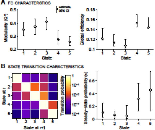
Characterization of FNC states (A) and transitions between them (B). (A) Estimates of modularity (left) and global efficiency (right) of each connectivity state. (B) The state transition matrix (TM) averaged over subjects (left), and the stationary probability vector (π, principal eigenvector of the TM, right) which shows steady-state, or “long-run” behavior. Note that transition probability is color-mapped on a log-scale. In all plots, error bars indicate the non-parametric 95% confidence intervals (CIs) of each quantity, obtained by resampling subjects and recalculating the quantity on bootstrapped sample (500 repetitions).

EEG spectra segregated by fMRI FNC states

EEG spectra from each TR were segregated into different groups based on concurrent FNC state vectors. FNC state vectors were aligned to EEG using the time point corresponding to the center of the sliding window. Differences between the segregated spectra were then quantified in two ways. First, we calculated the Euclidean distance between average state-specific spectra to obtain a single statistic summarizing all differences. Second, we calculated the difference between each state-specific amplitude and the global average (obtained over all subjects and epochs), at delta (1–4 Hz), theta (4–8 Hz), and alpha (8–12 Hz) frequency bands. This measure provides directional and spectral specificity regarding differences between states. For both methods, calculations were performed separately at each channel.

We used non-parametric permutation testing (Nichols and Holmes, 2002) to determine whether the observed differences measures between state-specific EEG spectra were greater than would be expected by chance; standard parametric models, such as an ANOVA, are challenging to implement here due the non-independence of neighboring windows and uneven sampling of states by different subjects. To create appropriate null distributions, fMRI FNC state vectors were permuted across subjects and shifted in time relative to the EEG data. Temporal shifts were drawn randomly from [−W/2, W/2] and values were shifted circularly. Such a permutation scheme maintains the autocorrelation structure of the original FNC state vectors and approximates transition statistics, but destroys EEG-fMRI synchrony within subjects as well as EEG-fMRI temporal trends that may be common across subjects. Difference measures between spectra were computed using the permuted state vectors to create null distributions, and p-values were determined by comparing observed statistics to the null (10,000 permutations). To facilitate visual comparisons in topographic displays, difference measures were converted to z-scores based on the mean and standard deviation of the null distributions at each channel.

Results

Figure 1A displays the ICNs identified with group ICA. Based on their anatomical and presumed functional properties, ICNs are arranged into groups of sub-cortical (SC), auditory (AUD), somatomotor (SM), visual (VIS), cognitive control (CC; referring loosely to the planning, monitoring, and adapting one’s behavior), default-mode (DM) and cerebellar (CB) components. Peak activations and coordinates of each component are provided in Table 1. Figure 1B displays the average static FNC between ICNs in the EO condition to facilitate visual comparison with our earlier work (see Fig. 2A of (Allen et al., 2012)).

Figure 1.

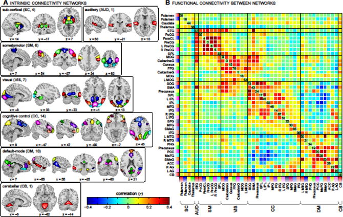
ICN spatial maps (A) and the static FNC between them (B), averaged across 23 subjects in the EO condition. ICNs are divided into groups and arranged based on their anatomical and functional properties. Within each group, the color of the component in (A) corresponds to the colored flag shown along the axes of (B). ICN labels in (B) denote the brain region(s) with peak amplitude and refer to bilateral homologues unless specified as left (L) or right (R). See Table 1 for peak coordinates in each component. STG = superior temporal gyrus; PoCG = postcentral gyrus; ParaCL = paracentral lobule; PreCG = precentral gyrs; SPL = superior parietal lobule; MOG = middle occipital gyrus; FFG = fusiform gyrus; SOG = superior occipital gyrus; SMA = supplementary motor area; IPL = inferior parietal lobule; MFG = middle frontal gyrus; IFG = inferior frontal gyrus; SFG = superior frontal gyrus; SMeG = superior medial gyrus; MTG = middle temporal gyrus; PHG = parahippocampal gyrus; PCC = posterior cingulate cortex; MeFG = medial frontal gyrus; ACC = anterior cingulate cortex; AG = angular gyrus; CB = cerebellum

Table 1.

Peak coordinates of ICNs

Intrinsic Connectivity Network	BA	Max (Z)	Peak (mm)
			x	y	z
Sub-cortical networks (4)	–	–	–	–	–
Putamen (28)
L putamen		9.8	−27	−4	7
R putamen		9.0	27	−1	4
Putamen (16)
R putamen	47	9.2	21	11	−8
L putamen	34	9.8	−24	8	−5
Caudate (44)
Bi caudate nucleus		11.8	−9	−1	13
Thalamus (36)
L thalamus		9.7	−12	−16	7
R thalamus		8.7	15	−16	7
Auditory networks (1)	–	–	–	–	–
STG (37)
R superior temporal gyrus	22	7.4	54	−13	4
L superior temporal gyrus	41	7.5	−57	−22	10
Somatomotor networks (6)	–	–	–	–	–
PoCG (35)
R postcentral gyrus	3	9.3	60	−22	37
L postcentral gyrus	1	6.6	−60	−28	40
ParaCL (4)
Bi paracentral lobule	6	9.8	0	−28	61
PreCG (2)
L precentral gyrus	6	10.6	−51	−13	34
R precentral gyrus	4	10.2	60	−4	25
L PreCG (6)
L precentral gyrus	4	10.6	−39	−25	61
R PreCG (5)
R precentral gyrus	4	9.6	39	−19	52
SPL (33)
L superior parietal lobule	7	7.7	−24	−58	61
R superior parietal lobule	7	6.4	24	−55	61
Visual networks (7)	–	–	–	–	–
MOG (9)
R middle occipital gyrus	19	10.1	51	−70	4
L middle occipital gyrus	19	7.8	−48	−79	1
CalcarineG (3)
Bi calcarine gyrus	17	9.1	−15	−64	4
Cuneus (15)
Bi cuneus	18	8.8	9	−97	25
FFG (76)
R fusiform gyrus	19	7.5	30	−49	−11
R superior occipital gyrus	19	7.0	33	−88	19
L fusiform gyrus	19	5.9	−27	−55	−11
CalcarineG (1)
Bi calcarine gyrus	17	9.3	3	−91	−2
MOG (18)
R middle occipital gyrus	18	9.8	27	−100	−2
L middle occipital gyrus	18	7.6	−27	−100	−5
L MOG (54)
L middle occipital gyrus	18	8.7	−33	−91	1
Cognitive control networks (14)		–	–	–	–
SOG (73)
L superior occipital gyrus	19	7.6	−27	−85	28
R superior occipital gyrus	19	6.2	36	−82	28
SMA (43)
Bi supplementary motor area	6	7.9	0	11	49
Precuneus (24)
Bi Precuneus	7	8.4	3	−61	55
SPL (17)
R superior parietal lobule	7	8.4	3	−61	55
L superior parietal lobule	7	5.5	−30	−67	55
L IPL (41)
L Inferior parietal lobule	40	8.6	−51	−40	43
IPL (63)
R inferior parietal lobule	40	9.8	63	−40	34
L inferior parietal lobule	40	6.3	−57	−52	37
MFG (46)
L middle frontal gyrus	10	7.7	−33	47	28
R middle frontal gyrus	10	5.0	30	47	22
IFG (14)
R inferior frontal gyrus	45	8.9	45	23	25
L inferior frontal gyrus	9	5.5	−45	14	34
R IFG (67)
R inferior frontal gyrus	47	7.3	48	47	−5
L middle orbital gyrus	10	6.4	−45	47	−5
L IFG (32)
L inferior frontal gyrus	45	8.4	−51	23	22
Bi SFG (25)
Bi superior frontal gyrus	6	6.7	15	20	61
MFG (30)
L middle frontal gyrus	10	9.5	−30	62	7
R middle frontal gyrus	10	5.7	27	53	4
SMeG (65)
superior medial gyrus	9	6.9	0	41	40
IFG (38)
L inferior frontal gyrus	47	7.9	−42	23	−11
R inferior frontal gyrus	47	6.8	45	26	−8
Default-mode networks (10)	–	–	–	–	–
L MTG (50)
L middle temporal gyrus	21	8.2	−60	−31	−2
R MTG (21)
R middle temporal gyrus	22	9.1	57	−43	10
PHG (34)
R parahippocampal gyrus	34	9.4	15	−1	−20
L parahippocampal gyrus	34	9.2	−12	−10	−20
Precuneus (19)
Bi precuneus	7	10.1	0	−76	34
PCC (70)
R posterior cingulate cortex	23	7.7	12	−58	16
R middle temporal gyrus	39	6.6	45	−70	22
L middle temporal gyrus	39	4.8	−39	−73	22
MeFG (29)
Bi medial frontal gyrus	11	7.7	0	32	−11
SMeG (53)
Bi superior medial gyrus	9	8.3	0	59	28
Bi precuneus	7	6.5	0	−61	34
ACC (26)
Bi anterior cingulate cortex	32	9.7	0	38	22
R AG (22)
R angular gyrus	40	8.2	51	−61	46
L AG (20)
L angular gyrus	40	9.1	−48	−64	43
Cerebellar networks (1)	–	–	–	–	–
CB (8)
Bi cerebellar vermis		9.2	0	−70	−14

Connectivity States

Clustering results with k = 5 are shown in Figure 2. FNC states are characterized by the cluster centroids (Fig. 2A) and their occurrence as a function of time (Fig. 2B). States are arranged in order of their temporal precedence, considering both EO and EC scans (see Methods). State 1 (S1) is characterized by highly modular FNC, with prominent connectivity among SM networks. It occurs throughout the EO condition but is almost completely absent during EC. S2 shows similar FNC (though little distinction of the SM module) and temporal trends, with decreased occurrence at later time points in the EO condition and relatively few occurrences in EC. S3 exhibits a different pattern in time, with a moderate presence during EO followed by a large jump in occurrence at the start of EC that decays over the duration of the scan. With regard to FNC, S3 shows VIS components less correlated to CC networks and more correlated to DM networks. FNC patterns of S4 and S5 differ considerably from S1‒S3. In S4, all primary sensorimotor and higher-modal association areas (AUD, SM, VIS, as well as some CC and DM components) are highly correlated, resulting in a reduction in modularity (Q*; Fig. 3A, left) and increase in global efficiency (E^W; Fig. 3A, right). Temporally, S4 exhibits a prominent linear increase during EO and then maintains a relatively constant presence during EC. S5 shows even greater “hypersynchronization””, as it lacks the antagonism/anticorrelation between SC and sensorimotor components seen in S4. Regarding occurrence, S5 is largely absent during EO but exhibits increasing presence throughout EC. Quantitative comparisons of within and between module connectivity assessments are provided in Supplemental Figure 2.

Figure 2.

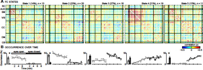
Clustering result for k = 5. Each cluster (State 1 to State 5) is summarized by its centroid (A), and occurrences as a function of time (B). The total percentage of occurrences (over EO and EC conditions) and the number of subjects that entered each state (n) is provided above each centroid. Bar plots in (B) compare the average occurrence in EO (light gray) and EC (dark gray) conditions. Error bars denote the standard error over subjects. Asterisks indicate a significant difference in state occurrence between EO and EC (P < 0.05, nonparametric permutation test, Bonferroni corrected for multiple comparisons). Dashed lines in (B) show the best linear fit to the occurrence trends.

Note that the removal of global mean signal prior to subject-specific PCA enforces the ICA decomposition space to be null space of global signal and introduces anti-correlations (Fox et al., 2009). The change in strength of connectivity from state to state still holds, however the sign change need to be interpreted with caution. Global signal removal is included in the PCA step in ICA framework. The removal of global signal (either regression or mean subtraction) has been intensely debated in the community and pros and cons are reviewed in detail in Power et al., 2015. The global mean subtraction referred to as frame-to-frame intensity stabilization removes a constant value per time point across all voxels unlike regression which removes weighted version of the global signal with different weighting per voxel. While both methods force the distribution of correlation around zero value, regression might introduce interregional biases in correlation estimates (Saad et al., 2012).

The temporal properties of FNC states can also be characterized by studying the transitions between states. Figure 3B (left) shows the average transition matrix (TM), representing the probability of changing from one state to another. White squares along the diagonal signify a very high probability of staying in the same state. Notably, the probability of transitioning from S2 to S3, P(S2 → S3), is larger than P(S3 → S2). Likewise, P(S3 → S4) is larger than P(S4 → S3), and P(S4 → S5) is greater than P(S5 → S4), conveying a directionality to the transitions. This notion is supported by the steady-state probability (π) computed from the TM, displayed in Figure 3B (right), which suggests that subjects are most likely to be found in S4 or S5 in the long run.

EEG segregation

To determine the electrophysiological signatures of different FNC states, EEG spectra computed over each 2 s TR were segregated into groups based on the FNC state label for the window centered on that TR (see Methods and Fig. 4A). The result of this segregation is shown in Figure 4B for central channel Cz (left) and occipital channels O1 and O2 (right). If the fMRI-derived FNC patterns were unrelated to electrophysiology, we would expect the spectra from different states to overlap with one-another. In contrast, we find large differences between the spectra, summarized as follows: S1 shows little synchronization in delta/theta ranges and a weak peak in the alpha band; S2 exhibits relatively greater alpha power over central but not occipital electrodes; S3 exhibits robust alpha synchronization, primarily over occipital electrodes but also extending more anteriorly; S4 shows alpha synchronization similar in magnitude to S2, though the alpha peak is broadened toward lower frequencies, and slower oscillations (< 7 Hz) are also present; S5 shows the most distinct electrophysiological profile, with strong and widespread synchronization at delta and theta frequencies and desynchronization of occipital alpha. Statistical differences between spectra were determined with Monte Carlo permutation tests (see Methods) and confirmed that spectral signatures of states at central electrodes were significantly (P < 0.01, FDR corrected) more distant from each other than would be expected by chance (Fig. 4D). Comparing state-specific amplitude to the global average also supported topographic and band-limited spectral differences (Supplementary Figure 3).

Figure 4.

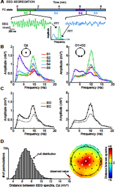
EEG spectra, segregated by FNC state. (A) A schematic illustrating EEG segregation for a single subject. Spectra are computed for each 2 s epoch of EEG data and are divided into groups based on the FNC state vector from the concurrent fMRI data. (B) EEG spectra averaged over all epochs and subjects, segregated by FNC state. For comparison, EEG spectra segregated by eye condition are shown in panel (C). (D) Determination of the statistical significance of EEG spectral segregation. In the left panel, an example of the observed total Euclidean distance between EEG spectra (red dot) is compared to the null distribution of distances (gray) obtained via Monte Carlo permutation testing (see Methods). To facilitate visual comparisons in topographic displays, difference measures were converted to z-scores based on the mean and standard deviation of the null distributions at each channel. Filled white electrodes in the topoplots signify P <0.01, FDR corrected for multiple comparisons over channels.

For comparison, EEG spectra segregated by behavioral state (EO vs EC) are shown in Figure 4C for the central and occipital electrodes. As expected (Berger, 1929; Santamaria and Chiappa, 1987), EC shows much greater posterior alpha power than EO, but also shows elevated delta and theta power over central electrodes, which is typically associated with reduced alertness (Åkerstedt et al., 1990; Laufs et al., 2006; Makeig and Inlow, 1993; Makeig and Jung, 1996) rather than eye-closing per se. The fMRI FC-driven segregation suggests a clear distinction between these electrophysiological signatures: alpha synchronization is associated with S3, which is most likely to occur at the onset of eye-closing (Fig. 2B), while increased delta and theta rhythms are strongly associated with S5, which is observed increasingly at later time points in the EC condition and possibly reflects N1 sleep stage. Thus, FNC-derived states appear to provide better segregation of EEG signatures than the observed behavioral states.

Figure 5 shows the FNC states and corresponding EEG spectra for three representative subjects. Non-stationarities in EEG spectra are clearly visible, particularly in subjects 7 and 17 who undergo alpha desynchronization 1–2 minutes after eye-closing, and FNC dynamics are evident. The average state-specific spectra for each subject (left, upper panels in Fig. 5A–C) show trends that resemble the group results displayed in Figure 4B. Importantly, while these examples show that state-specific EEG and FNC patterns found at the group level can also be seen at the level of the individual, they also illustrate the high degree of variability between subjects (e.g., windows classified as S4 in subject 7 show many differences from those classified as S4 in subject 17) as well as within subjects (e.g., windows classified as S4 in subject 17 during EO share limited features with those classified as S4 in EC). These issues are addressed further in the Discussion.

Figure 5.

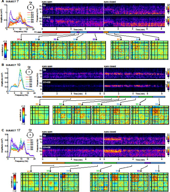
Examples of EEG spectra and FNC dynamics for subject 7 (A), subject 10 (B), and subject 17 (C). For each subject, the upper panels display EEG spectrograms for EO and EC conditions at central (Cz) and occipital (O1 + O2) electrodes. Lower panels display dynamic FNC matrices, averaged over contiguous windows that are clustered into the same state. FNC state assignments are denoted with different colors beneath the spectrograms. The upper left panel displays average EEG power at Cz, segregated by FNC state, in the same format as Figure 3B.

Discussion

In this work we successfully replicate our earlier findings on the presence of distinct FNC connectivity states in resting conditions, which reoccur within and across subjects, obtained from clustering of sliding windowed correlation matrices. Even in a much smaller sample compared to our previous study, two of the three states obtained in EO condition resemble those obtained from that study. The state S4 from current study is comparable to state S3 in previous analysis exhibiting similar thalamo-cortical antagonism and increased frequency with time in EO condition. Also state S2 in current study resembles state S7 from earlier study and shows similar decrease in frequency of occurrence as scan progresses in EO condition. Additionally, we show that these FNC states correspond to neuro-electric brain activity with distinct EEG spectral signatures validating our approach to estimate connectivity dynamics despite its shortcomings (see limitations). The state S4 which we speculated to be associated with decrease in vigilance in fact exhibits increase in delta and theta power in EEG spectrum along with a decrease in alpha power compared to EO awake state S1, a well-established characteristic of reduced vigilance (Makeig and Jung, 1995). These transitions from more alert state to less alert state (and probably light sleep) occurs gradually as scan progresses, which is in good agreement with (Olbrich et al., 2009; Tagliazucchi and Laufs, 2014). Recent sleep classification study using fMRI resting data also observed that the subcortical-cortical connections are more discriminatory in awake to sleep stage1 transition (Altmann et al., 2016).

In some ways, the current work represents the inverted/reverse approach to (Tagliazucchi and Laufs, 2014; Tagliazucchi et al., 2012). Long periods (hours) of concurrent EEG-fMRI recordings, the authors first sleep-scored EEG into corresponding sleep stages, then used these labels to train FNC-based sleep-stage classifiers in a supervised learning framework. Here, rather than start with manual sorting and labelling of EEG, we use an unsupervised learning approach (k-means) to identify and segregate FNC patterns, then examined EEG spectra based on these classifications. Despite different goals and assumptions these approaches arrive at a number of similar conclusions regarding the changes in FNC associated with different EEG patterns: (1) Sleep staging of EEG data suggests that subjects are more likely to get into drowsy states and early sleep stages during EC condition than EC condition. EEG spectra from 20 of 23 subjects in EO condition depict strong alpha power suggesting vigilant state throughout the scan. Only a mix of slow theta and alpha waves with no evidence of vertex sharp waves in the rest of three subjects during EO scan suggesting a reduced vigilance state and/or reaching a slightly drowsy (sleep stage 1) state. In contrast, during EC scan, 12 out of 23 subjects exhibit prominent alpha power in their EEG spectra throughout the scan. In the rest of the subjects, as scan progresses, subjects show a shift of EEG power from higher alpha to a mix of alpha and theta. (2) Perhaps the most prominent feature of transition into sleep is the change in thalamo-cortical connectivity from positive correlation to anti-correlation, which we previously described in Allen et al., 2014 as “cortical-subcortical antagonism”. This is particularly consistent with Spoormaker et al., who additionally show that negative correlation between thalamus and cortex are most notable in the first stages of sleep, and diminish as individuals transition to deeper sleep (Spoormaker et al., 2010). However, a state with similar thalamo-cortical antagonism has been shown to be a signature of loss of arousal in resting state by Chang and colleagues using simultaneous fMRI and intracortical electrophysiological recordings in macaques (Chang et al., 2016). Therefore, future studies should investigate if there are specific differences between states corresponding to drop in arousal versus drowsiness.

The relationship of the thalamus and functional connectivity to other regions is particularly interesting as it is known to play important role in consciousness and exhibits distinct electrophysiological signatures during EO and EC states. Previous studies found that the thalamus is involved in coordinating alpha rhythm (Hughes and Crunelli, 2005). Our study supports the view that the thalamus plays an important role in terms of governing/tuning spontaneous alpha band signals, however it behaves as a sophisticated thalamo-cortical chronnectome system, rather than an isolated ‘pacemaker’. The transmission of sensory information to cortex from the thalamus is state-dependent, i.e. it is significantly reduced during drowsiness or fatigue while enhanced during vigilance, which may cause the observation of large anti-connectivity of thalamo-cortex in state 4 from our study. McCormick et al. showed that the transfer performance of corticothalamic fibers impacted how the cerebral cortex ‘gates or controls selective fields of sensory inputs in a manner that facilitates arousal, attention, and cognition’ (McCormick and von Krosigk, 1992). Nevertheless, the correspondence between posterior alpha and the ‘drowsy FNC signature’ (state 4) that we found needs further investigations.

In this work, we utilize EO and EC conditions that correspond to distinct neurophysiological state with EO state representing more aware “exteroceptive” state characterized by overt attention and oculomotor activity, while EO state corresponds to more “interoceptive” state characterized by imagination and multisensory activity (Hüfner et al., 2009, 2008) and have been recently been shown to correspond to different functional topologies (Jao et al., 2013; Xu et al., 2014). Our observations of greater integration within sensory systems during EC compared to EO condition, as seen in S4, are consistent with the earlier reports (Bianciardi et al., 2009; Xu et al., 2014). Furthermore, as reported by Xu and colleagues, we observe reduced modularity and increased global efficiency during EC condition (Figure 3A and 3B) compared to EO condition. The greater modularity in EO condition is thought to facilitate increased local efficiency during exteroceptive processing.

In a concurrent EEG-fMRI sleep study, Tagliazucchi et al. presented compelling evidence for increased network modularity in N3 stage sleep as compared to wakefulness, but no change from wakefulness to N1 sleep, and demonstrated positive covariation between delta band power and modularity, and negative covariation between alpha power and modularity (Tagliazucchi et al., 2013a). Also Boly et al, 2012 report similar modularity increases specific to deeper sleep (Boly et al., 2012). However, our current findings show decreased network modularity in S4 and S5 as compared to S1–3 (see Figure 3A). In combination with (Spoormaker et al., 2011, 2010), our results suggest that due to increased inter-module connections, modularity decreases with drowsiness in light sleep conditions. Modularity then increases substantially as subjects attain deep sleep and cortico-cortico connectivity is significantly reduced, (Boly et al., 2012; Tagliazucchi et al., 2013b) is consistent with TMS and notions of sleep. Increase in positive functional connectivity (and loss of inter-modular negative correlations) in the descent to light sleep is not well understood, though Spoormaker and colleagues hypothesize it reflects more random network organization that interferes with information integration (Spoormaker et al., 2011).

Decreased modularity in these states is congruent with visual comparisons of the FNC centroids displayed in Figure 2A; compared to S1–3, S4 and S5 exhibit more strong positive connections between larger sets of ICNs, and many fewer negative correlations between well-defined modules. Thus it is visually more difficult to subdivide ICNs into clearly delineated groups, consistent with lower modularity scores. Though analogous visualizations are not available for inspection in (Tagliazucchi et al., 2013a), one possible reason for the apparent contradiction between studies is the use of a different modularity metrics. Here, we use Q*, based on the definitions provided by Rubinov and Sporns, which considers both positive and negative weights of the unthresholded connectivity matrix (Rubinov and Sporns, 2011). Tagliazucchi et al. use Q, which considers only the positive elements of a thresholded connectivity matrix. As shown in Figure 1 of (Rubinov and Sporns, 2011), for a given network with fixed intra-module connections, increasing the presence of inter-module negative connections will increase Q* values but decrease Q values; thus it is possible that differences in modularity estimates are related to sensitivity (or lack thereof) to inter-module negative correlations.

Implications for future work

Combined with previous work, the current results advocate a more rigorous characterization of subject states when assessing functional connectivity. Describing an “eyes-closed resting-state” is unlikely to sufficiently describe the changes in vigilance states subjects may experience, even during relatively short experiments. As demonstrated comprehensively by Tagliazucchi and Laufs, when scanning participants with EC, a loss of wakefulness should be expected in a third of subjects after 4 minutes of rest, and nearly half of subjects after 10 minutes (Tagliazucchi and Laufs, 2014). In particular, one should be wary of comparing subject groups that may exhibit different resting behavior (e.g., are more or less likely to become drowsy due to anxiety, medication, comfort, etc.). A dynamic FNC analysis that segregates time periods into different states and then analyzes the FNC within states may circumvent this problem, an approach we have applied in a recent study examining resting-state FNC in Schizophrenia (Damaraju et al., 2014). We found that segregating FNC states (and therefore, likely cognitive and vigilance states) prior to group comparisons yielded more specific group differences in connectivity and revealed additional differences that were obfuscated in stationary FNC comparisons.

Topological descriptions are very useful to condense networks into summary properties, but one should be careful not to use them as a substitute for examining the networks themselves. For example, the modularity and global efficiency of states 4 and 5 are not statistically different, however the networks themselves and occurrence profiles show profound differences.

This work also suggests caution in interpreting observed FC/FNC dynamics as shifts in cognition. This is not to say that FC changes are not sensitive to changes in internal behaviors, which have been demonstrated unequivocally (Gonzalez-Castillo et al., 2015; Shirer et al., 2012). However, in the absence of any experimentally guided behaviors (recollecting events, silent humming), subjects are likely to do a large number of very different things [unknown to the experimenter]. In terms of data-driven analysis, it is likely, then, that many large sources of variance will be related to vigilance shifts (Czisch et al., 2012; Olbrich et al., 2009). Wong et al, 2013 show that this time-varying decreases of vigilance, as evidenced by increases in delta and theta spectral EEG power, exhibits an inverse relationship to global signal amplitude (and therefore functional connectivity) and argue that global signal regression performed in seed-based connectivity approaches probably reduces the variance associated with vigilance shifts across subjects to certain extent (Wong et al., 2016, 2013). Similar results to Wong and colleagues (Wong et al., 2013, 2012), showing a strong relationship between EEG measures of vigilance and the amplitude of the global signal (which is related to antagonism), we observe that states S4 and S5 show a marked reduction in the number of negative inter-modular connections, which is directly related to the amplitude of the global signal.

Comparisons to Other EEG-fMRI Integration Approaches

Until recently the majority of EEG-fMRI integration studies have focused on amplitude modulations, i.e., change in band-limited power in EEG is expected to relate to change in BOLD signal (Laufs et al., 2008). This is perhaps the most reasonable model given the established causative relationship between neural activation and hemodynamic response (Logothetis, 2008; Mukamel et al., 2005). However, neural signaling need not involve the changes in the amplitude power of on ongoing oscillations. A number of investigations show that functional networks are formed by phase relationships between distant neural populations as well as cross frequency coupling (Canolty et al., 2006; Montemurro et al., 2008) spurring the development of alternative models that consider the relationship between electrophysiological signals and fMRI-derived FC.

Several studies have considered time-varying FC as a function of EEG power: Using psychophysiological interaction analysis using low and high alpha power segments as intrinsic task condition, Scheeringa and colleagues report reduced FC within visual cortex with increases in alpha power and reductions in anti-correlation with thalamus (Scheeringa et al., 2012). Using sliding window analysis, Chang and colleagues demonstrate time-varying connectivity between default-mode network and dorsal attention network whose strength is inversely correlated with alpha power potentially reflecting state dependent dynamics (Chang et al., 2013). Using a similar analysis but extended to whole brain regions of interest, Tagliazucchi and colleagues investigate dynamic FC electrophysiological correlates by and report decreases in FC with increases in alpha and beta EEG spectral power and increases in dynamic FC with theta power increases (Tagliazucchi et al., 2012).

Here, we use a similar approach but use clustering of the fMRI-FC to segregate time windows, removing the assumption of a linear relationship between FNC and EEG power. Some advantages of our approach: (1) inherently multivariate, so doesn’t (erroneously) consider correlations between brain regions as independent quantities. (2) Doesn’t suffer from a multiple comparison issue (i.e., testing correlations between all brain regions separately. (3) perhaps most importantly does not assume that the relationship between EEG power and FNC is static thereby has better ability to capture dynamic reconfiguration of network connections both with vigilance shifts as well as internal behaviors.

Limitations

Because both FNC and EEG show systematic changes over time (and with EO/EC) it’s possible that we are vastly overestimating any “link” between the two modalities. Despite capturing dynamic connectivity reconfiguration, one can expect to lose some detail with clustering, as estimates of FNC using shorter windowed time series can be noisy, and focusing on FNC states/centroids results in some loss of specificity between single regions in some cases. Furthermore, a great deal of subject heterogeneity is lost in the k-means approach – e.g., in Fig. 5, the S4 in individual subjects are different. We observed that subjects tend to “drowsy FNC states” sooner in EC condition than EO condition. This is consistent with earlier reports that suggest increased likelihood of falling asleep in eyes closed state than eyes open state in general (Tagliazucchi and Laufs, 2014), however, we could not rule out the possibility that this could be due to the fact that EC scan was performed later than EO scans for all subjects and the subjects are likely more tired by the EC scan time as the scan order was not counterbalanced. Obvious large confound is motion. Though we have tried to minimize the influence of motion by using ICA and regressing motion-derived signals from the timecourses of components of interest based on a previous study of motion effects in ICA (Damaraju et al., 2014), we cannot eliminate the possibility that residual motion-related variance has impacted the FNC estimates (Laumann et al., 2016). Also, some of the choices made for example model order selection in ICA, window length for dFNC estimation are subjective, however the settings we did use have given consistent results across many different datasets. Despite this the empirical choices should still continue to be explored in future work.

Conclusions

In this work we demonstrate that dynamic FNC states estimated using k-means clustering of correlations estimated using sliding windowed ICA time courses results in meaningful clusters that correspond to distinct electrophysiological mental states. Our work supports the earlier works that simultaneously acquiring EEG with functional MRI data can provide complementary information that enables the investigator to make informed inferences about observed FNC dynamics. As evidenced by EEG spectral signatures associated with FNC states, our data suggests that evaluation of drowsiness is important in both eyes open and eyes closed resting state conditions and researchers should carefully account for these when comparing different populations. Although dynamic FNC estimation using sliding-window technique can be noisy, we can be relatively confident that the FNC dynamics estimated using this method reflect, to some degree, changes in local and distal neural coherence(Berger, 1929).

Supplementary Material

10548_2017_546_MOESM1_ESM

Supplementary Figure 1. A) Outline of fMRI processing steps. B) Schematic depicting ICA decomposition to obtain subject-specific spatial maps and corresponding time courses. C) Schematic depicting dynamic functional connectivity estimation and subsequent k-means clustering procedure to obtain subject state vector.

10548_2017_546_MOESM2_ESM

Supplementary Figure 2. Quantitative comparisons summarizing modular connectivity differences between states. The mean correlations between and within modules are computed for windows corresponding to each state and averaged across time for each subject. These subject means are then compared using one-way ANOVA and subsequent two-sample t-tests to test for significant differences in connectivity among modules across different states. *, ◊,○,Δ-represent significant difference in mean correlation of the state with state 1, 2, 3 and 4 respectively.

10548_2017_546_MOESM3_ESM

Supplementary Figure 3. Differences between EEG state spectra and the global mean, as a function of band. Difference measures between spectra were computed using the permuted state vectors to create null distributions, and p-values were determined by comparing observed statistics to the null (10,000 permutations).

References

- Åkerstedt T, Arnetz BB, Anderzén I. Physicians during and following night call duty—41 hour ambulatory recording of sleep. Electroencephalogr Clin Neurophysiol. 1990;76:193–196. doi: 10.1016/0013-4694(90)90217-8. [DOI] [PubMed] [Google Scholar]
- Allen EA, Damaraju E, Plis SM, Erhardt EB, Eichele T, Calhoun VD. Tracking Whole-Brain Connectivity Dynamics in the Resting State. Cereb Cortex. 2012 doi: 10.1093/cercor/bhs352. [DOI] [PMC free article] [PubMed] [Google Scholar]
- Allen EA, Erhardt EB, Damaraju E, Gruner W, Segall JM, Silva RF, Havlicek M, Rachakonda S, Fries J, Kalyanam R, Michael AM, Caprihan A, Turner JA, Eichele T, Adelsheim S, Bryan AD, Bustillo J, Clark VP, Feldstein Ewing SW, Filbey F, Ford CC, Hutchison K, Jung RE, Kiehl KA, Kodituwakku P, Komesu YM, Mayer AR, Pearlson GD, Phillips JP, Sadek JR, Stevens M, Teuscher U, Thoma RJ, Calhoun VD. A baseline for the multivariate comparison of resting-state networks. Front Syst Neurosci. 2011;5:2. doi: 10.3389/fnsys.2011.00002. [DOI] [PMC free article] [PubMed] [Google Scholar]
- Allen PJ, Josephs O, Turner R. A method for removing imaging artifact from continuous EEG recorded during functional MRI. Neuroimage. 2000;12:230–9. doi: 10.1006/nimg.2000.0599. [DOI] [PubMed] [Google Scholar]
- Altmann A, Schröter MS, Spoormaker VI, Kiem SA, Jordan D, Ilg R, Bullmore ET, Greicius MD, Czisch M, Sämann PG. Validation of non-REM sleep stage decoding from resting state fMRI using linear support vector machines. Neuroimage. 2016;125:544–555. doi: 10.1016/j.neuroimage.2015.09.072. [DOI] [PubMed] [Google Scholar]
- Barry RJ, Clarke AR, Johnstone SJ, Magee CA, Rushby JA. EEG differences between eyes-closed and eyes-open resting conditions. Clin Neurophysiol. 2007;118:2765–2773. doi: 10.1016/j.clinph.2007.07.028. [DOI] [PubMed] [Google Scholar]
- Bell AJ, Sejnowski TJ. An information-maximization approach to blind separation and blind deconvolution. Neural Comput. 1995;7:1129–59. doi: 10.1162/neco.1995.7.6.1129. [DOI] [PubMed] [Google Scholar]
- Berger H. Über das elektrenkephalogramm des menschen. Eur Arch Psychiatry Clin Neurosci. 1929;87:527–570. [Google Scholar]
- Bianciardi M, Fukunaga M, van Gelderen P, Horovitz SG, de Zwart JA, Duyn JH. Modulation of spontaneous fMRI activity in human visual cortex by behavioral state. Neuroimage. 2009;45:160–168. doi: 10.1016/j.neuroimage.2008.10.034. [DOI] [PMC free article] [PubMed] [Google Scholar]
- Boly M, Perlbarg V, Marrelec G, Schabus M, Laureys S, Doyon J, Pélégrini-Issac M, Maquet P, Benali H. Hierarchical clustering of brain activity during human nonrapid eye movement sleep. Proc Natl Acad Sci U S A. 2012;109:5856–61. doi: 10.1073/pnas.1111133109. [DOI] [PMC free article] [PubMed] [Google Scholar]
- Bridwell DA, Wu L, Eichele T, Calhoun VD. The spatiospectral characterization of brain networks: Fusing concurrent EEG spectra and fMRI maps. Neuroimage. 2013;69:101–111. doi: 10.1016/j.neuroimage.2012.12.024. [DOI] [PMC free article] [PubMed] [Google Scholar]
- Buzsaki G. Rhythms of the Brain. Oxford University Press; 2006. [Google Scholar]
- Calhoun VD, Adali T. Multisubject independent component analysis of fMRI: a decade of intrinsic networks, default mode, and neurodiagnostic discovery. Biomed Eng IEEE Rev. 2012;5:60–73. doi: 10.1109/RBME.2012.2211076. [DOI] [PMC free article] [PubMed] [Google Scholar]
- Calhoun VD, Adali T, Pearlson GD, Pekar JJ. A method for making group inferences from functional MRI data using independent component analysis. Hum Brain Mapp. 2001;14:140–51. doi: 10.1002/hbm.1048. [DOI] [PMC free article] [PubMed] [Google Scholar]
- Calhoun VD, Miller R, Pearlson G, Adalı T. The chronnectome: time-varying connectivity networks as the next frontier in fMRI data discovery. Neuron. 2014;84:262–274. doi: 10.1016/j.neuron.2014.10.015. [DOI] [PMC free article] [PubMed] [Google Scholar]
- Canolty RT, Edwards E, Dalal SS, Soltani M, Nagarajan SS, Kirsch HE, Berger MS, Barbaro NM, Knight RT. High Gamma Power Is Phase-Locked to Theta Oscillations in Human Neocortex. Sci. 2006;313:1626–1628. doi: 10.1126/science.1128115. [DOI] [PMC free article] [PubMed] [Google Scholar]
- Chang C, Glover GH. Time-frequency dynamics of resting-state brain connectivity measured with fMRI. Neuroimage. 2010;50:81–98. doi: 10.1016/j.neuroimage.2009.12.011. [DOI] [PMC free article] [PubMed] [Google Scholar]
- Chang C, Leopold DA, Schölvinck ML, Mandelkow H, Picchioni D, Liu X, Frank QY, Turchi JN, Duyn JH. Tracking brain arousal fluctuations with fMRI. Proc Natl Acad Sci. 2016 doi: 10.1073/pnas.1520613113. 201520613. [DOI] [PMC free article] [PubMed] [Google Scholar]
- Chang C, Liu Z, Chen MC, Liu X, Duyn JH. EEG correlates of time-varying BOLD functional connectivity. Neuroimage. 2013;72C:227–236. doi: 10.1016/j.neuroimage.2013.01.049. [DOI] [PMC free article] [PubMed] [Google Scholar]
- Cordes D, Haughton VM, Arfanakis K, Carew JD, Turski PA, Moritz CH, Quigley MA, Meyerand ME. Frequencies contributing to functional connectivity in the cerebral cortex in “resting-state” data. Am J Neuroradiol. 2001;22:1326–1333. [PMC free article] [PubMed] [Google Scholar]
- Czisch M, Wehrle R, Harsay HA, Wetter TC, Holsboer F, Sämann PG, Drummond SPA. On the Need of Objective Vigilance Monitoring: Effects of Sleep Loss on Target Detection and Task-Negative Activity Using Combined EEG/fMRI. Front Neurol. 2012;3:67. doi: 10.3389/fneur.2012.00067. [DOI] [PMC free article] [PubMed] [Google Scholar]
- Damaraju E, Allen EA, Belger A, Ford JM, McEwen S, Mathalon DH, Mueller BA, Pearlson GD, Potkin SG, Preda A. Dynamic functional connectivity analysis reveals transient states of dysconnectivity in schizophrenia. NeuroImage Clin. 2014;5:298–308. doi: 10.1016/j.nicl.2014.07.003. [DOI] [PMC free article] [PubMed] [Google Scholar]
- Damaraju E, Allen EA, Calhoun VD. Impact of head motion on ICA-derived functional connectivity measures. Fourth Biennial Conference on Resting State; Boston. 2014. [Google Scholar]
- Delorme A, Makeig S. EEGLAB: an open source toolbox for analysis of single-trial EEG dynamics including independent component analysis. J Neurosci Methods. 2004;134:9–21. doi: 10.1016/j.jneumeth.2003.10.009. [DOI] [PubMed] [Google Scholar]
- Erhardt EB, Rachakonda S, Bedrick EJ, Allen EA, Adali T, Calhoun VD. Comparison of multi-subject ICA methods for analysis of fMRI data. Hum Brain Mapp. 2011;32:2075–2095. doi: 10.1002/hbm.21170. [DOI] [PMC free article] [PubMed] [Google Scholar]
- Fox MD, Zhang D, Snyder AZ, Raichle ME. The global signal and observed anticorrelated resting state brain networks. J Neurophysiol. 2009;101:3270–3283. doi: 10.1152/jn.90777.2008. [DOI] [PMC free article] [PubMed] [Google Scholar]
- Gonzalez-Castillo J, Handwerker DA, Robinson ME, Hoy CW, Buchanan LC, Saad ZS, Bandettini PA. The spatial structure of resting state connectivity stability on the scale of minutes. Front Neurosci. 2014;8:138. doi: 10.3389/fnins.2014.00138. [DOI] [PMC free article] [PubMed] [Google Scholar]
- Gonzalez-Castillo J, Hoy CW, Handwerker DA, Robinson ME, Buchanan LC, Saad ZS, Bandettini PA. Tracking ongoing cognition in individuals using brief, whole-brain functional connectivity patterns. Proc Natl Acad Sci. 2015;112:8762–8767. doi: 10.1073/pnas.1501242112. [DOI] [PMC free article] [PubMed] [Google Scholar]
- Handwerker DA, Roopchansingh V, Gonzalez-Castillo J, Bandettini PA. Periodic changes in fMRI connectivity. Neuroimage. 2012 doi: 10.1016/j.neuroimage.2012.06.078. [DOI] [PMC free article] [PubMed] [Google Scholar]
- Himberg J, Hyvärinen A, Esposito F. Validating the independent components of neuroimaging time series via clustering and visualization. Neuroimage. 2004;22:1214–1222. doi: 10.1016/j.neuroimage.2004.03.027. [DOI] [PubMed] [Google Scholar]
- Hüfner K, Stephan T, Flanagin VL, Deutschländer A, Stein A, Kalla R, Dera T, Fesl G, Jahn K, Strupp M. Differential effects of eyes open or closed in darkness on brain activation patterns in blind subjects. Neurosci Lett. 2009;466:30–34. doi: 10.1016/j.neulet.2009.09.010. [DOI] [PubMed] [Google Scholar]
- Hüfner K, Stephan T, Glasauer S, Kalla R, Riedel E, Deutschländer A, Dera T, Wiesmann M, Strupp M, Brandt T. Differences in saccade-evoked brain activation patterns with eyes open or eyes closed in complete darkness. Exp brain Res. 2008;186:419–430. doi: 10.1007/s00221-007-1247-y. [DOI] [PubMed] [Google Scholar]
- Hughes SW, Crunelli V. Thalamic mechanisms of EEG alpha rhythms and their pathological implications. Neurosci. 2005;11:357–372. doi: 10.1177/1073858405277450. [DOI] [PubMed] [Google Scholar]
- Huster RJ, Debener S, Eichele T, Herrmann CS. Methods for simultaneous EEG-fMRI: an introductory review. J Neurosci. 2012;32:6053–6060. doi: 10.1523/JNEUROSCI.0447-12.2012. [DOI] [PMC free article] [PubMed] [Google Scholar]
- Hutchison RM, Womelsdorf T, Gati JS, Everling S, Menon RS. Resting‐state networks show dynamic functional connectivity in awake humans and anesthetized macaques. Hum Brain Mapp. 2012 doi: 10.1002/hbm.22058. [DOI] [PMC free article] [PubMed] [Google Scholar]
- Jafri MJ, Pearlson GD, Stevens M, Calhoun VD. A method for functional network connectivity among spatially independent resting-state components in schizophrenia. Neuroimage. 2008;39:1666. doi: 10.1016/j.neuroimage.2007.11.001. [DOI] [PMC free article] [PubMed] [Google Scholar]
- Jao T, Vértes PE, Alexander-Bloch AF, Tang IN, Yu YC, Chen JH, Bullmore ET. Volitional eyes opening perturbs brain dynamics and functional connectivity regardless of light input. Neuroimage. 2013;69:21–34. doi: 10.1016/j.neuroimage.2012.12.007. [DOI] [PMC free article] [PubMed] [Google Scholar]
- Keilholz SD, Magnuson ME, Pan WJ, Willis M, Thompson GJ. Dynamic properties of functional connectivity in the rodent. Brain Connect. 2013;3:31–40. doi: 10.1089/brain.2012.0115. [DOI] [PMC free article] [PubMed] [Google Scholar]
- Laufs H, Daunizeau J, Carmichael DW, Kleinschmidt A. Recent advances in recording electrophysiological data simultaneously with magnetic resonance imaging. Neuroimage. 2008;40:515–528. doi: 10.1016/j.neuroimage.2007.11.039. [DOI] [PubMed] [Google Scholar]
- Laufs H, Holt JL, Elfont R, Krams M, Paul JS, Krakow K, Kleinschmidt A. Where the BOLD signal goes when alpha EEG leaves. Neuroimage. 2006;31:1408–1418. doi: 10.1016/j.neuroimage.2006.02.002. doi: http://dx.doi.org/10.1016/j.neuroimage.2006.02.002. [DOI] [PubMed] [Google Scholar]
- Laumann TO, Snyder AZ, Mitra A, Gordon EM, Gratton C, Adeyemo B, Gilmore AW, Nelson SM, Berg JJ, Greene DJ, McCarthy JE, Tagliazucchi E, Laufs H, Schlaggar BL, Dosenbach NUF, Petersen SE. On the Stability of BOLD fMRI Correlations. Cereb Cortex. 2016 doi: 10.1093/cercor/bhw265. [DOI] [PMC free article] [PubMed] [Google Scholar]
- Lindquist MA, Xu Y, Nebel MB, Caffo BS. Evaluating dynamic bivariate correlations in resting-state fMRI: a comparison study and a new approach. Neuroimage. 2014;101:531–46. doi: 10.1016/j.neuroimage.2014.06.052. [DOI] [PMC free article] [PubMed] [Google Scholar]
- Lloyd SP. Least squares quantization in PCM. Inf Theory IEEE Trans. 1982;28:129–137. [Google Scholar]
- Logothetis NK. What we can do and what we cannot do with fMRI. Nature. 2008;453:869–878. doi: 10.1038/nature06976. [DOI] [PubMed] [Google Scholar]
- Makeig S, Inlow M. Lapse in alertness: coherence of fluctuations in performance and EEG spectrum. Electroencephalogr Clin Neurophysiol. 1993;86:23–35. doi: 10.1016/0013-4694(93)90064-3. [DOI] [PubMed] [Google Scholar]
- Makeig S, Jung TP. Tonic, phasic, and transient EEG correlates of auditory awareness in drowsiness. Cogn Brain Res. 1996;4:15–25. doi: 10.1016/0926-6410(95)00042-9. [DOI] [PubMed] [Google Scholar]
- Makeig S, Jung TP. Changes in alertness are a principal component of variance in the EEG spectrum. Neuroreport. 1995;7:213–216. [PubMed] [Google Scholar]
- McCormick DA, von Krosigk M. Corticothalamic activation modulates thalamic firing through glutamate “metabotropic” receptors. Proc Natl Acad Sci U S A. 1992;89:2774–2778. doi: 10.1073/pnas.89.7.2774. [DOI] [PMC free article] [PubMed] [Google Scholar]
- Meyer CD. Matrix analysis and applied linear algebra. Siam 2000 [Google Scholar]
- Miller RL, Yaesoubi M, Turner JA, Mathalon DH, Preda A, Pearlson GD, Adali T, Calhoun VD. Higher Dimensional Meta-State Analysis Reveals Reduced Resting fMRI Connectivity Dynamism in Schizophrenia Patients. PLoS One. 2016 doi: 10.1371/journal.pone.0149849. [DOI] [PMC free article] [PubMed] [Google Scholar]
- Montemurro MA, Rasch MJ, Murayama Y, Logothetis NK, Panzeri S. Phase-of-firing coding of natural visual stimuli in primary visual cortex. Curr Biol. 2008;18:375–80. doi: 10.1016/j.cub.2008.02.023. [DOI] [PubMed] [Google Scholar]
- Mukamel R, Gelbard H, Arieli A, Hasson U, Fried I, Malach R. Coupling between neuronal firing, field potentials, and FMRI in human auditory cortex. Science (80−.) 2005;309:951–954. doi: 10.1126/science.1110913. [DOI] [PubMed] [Google Scholar]
- Niazy RK, Beckmann CF, Iannetti GD, Brady JM, Smith SM. Removal of FMRI environment artifacts from EEG data using optimal basis sets. Neuroimage. 2005;28:720–737. doi: 10.1016/j.neuroimage.2005.06.067. [DOI] [PubMed] [Google Scholar]
- Nichols TE, Holmes AP. Nonparametric permutation tests for functional neuroimaging: a primer with examples. Hum Brain Mapp. 2002;15:1–25. doi: 10.1002/hbm.1058. [DOI] [PMC free article] [PubMed] [Google Scholar]
- Olbrich S, Mulert C, Karch S, Trenner M, Leicht G, Pogarell O, Hegerl U. EEG-vigilance and BOLD effect during simultaneous EEG/fMRI measurement. Neuroimage. 2009;45:319–32. doi: 10.1016/j.neuroimage.2008.11.014. [DOI] [PubMed] [Google Scholar]
- Power JD, Schlaggar BL, Petersen SE. Recent progress and outstanding issues in motion correction in resting state fMRI. Neuroimage. 2015;105:536–551. doi: 10.1016/j.neuroimage.2014.10.044. [DOI] [PMC free article] [PubMed] [Google Scholar]
- Preti MG, Haller S, Giannakopoulos P, Van De Ville D. Decomposing dynamic functional connectivity onto phase-dependent eigenconnectivities using the Hilbert transform. Biomedical Imaging (ISBI), 2015 IEEE 12th International Symposium on. 2015:38–41. doi: 10.1109/ISBI.2015.7163811. [DOI] [Google Scholar]
- Rubinov M, Sporns O. Weight-conserving characterization of complex functional brain networks. Neuroimage. 2011;56:2068–2079. doi: 10.1016/j.neuroimage.2011.03.069. [DOI] [PubMed] [Google Scholar]
- Rubinov M, Sporns O. Complex network measures of brain connectivity: uses and interpretations. Neuroimage. 2010;52:1059–1069. doi: 10.1016/j.neuroimage.2009.10.003. [DOI] [PubMed] [Google Scholar]
- Saad ZS, Gotts SJ, Murphy K, Chen G, Jo HJ, Martin A, Cox RW. Trouble at rest: how correlation patterns and group differences become distorted after global signal regression. Brain Connect. 2012;2:25–32. doi: 10.1089/brain.2012.0080. [DOI] [PMC free article] [PubMed] [Google Scholar]
- Sakoğlu Ü, Pearlson GD, Kiehl KA, Wang YM, Michael AM, Calhoun VD. A method for evaluating dynamic functional network connectivity and task-modulation: application to schizophrenia. Magn Reson Mater Physics, Biol Med. 2010;23:351–366. doi: 10.1007/s10334-010-0197-8. [DOI] [PMC free article] [PubMed] [Google Scholar]
- Santamaria J, Chiappa KH. The EEG of drowsiness in normal adults. J Clin Neurophysiol. 1987;4:327–382. doi: 10.1097/00004691-198710000-00002. [DOI] [PubMed] [Google Scholar]
- Scheeringa R, Petersson KM, Kleinschmidt A, Jensen O, Bastiaansen MCM. EEG alpha power modulation of FMRI resting-state connectivity. Brain Connect. 2012;2:254–264. doi: 10.1089/brain.2012.0088. [DOI] [PMC free article] [PubMed] [Google Scholar]
- Shine JM, Oluwasanmi K, Bell PT, Gorgolewski KJ, Gilat M, Poldrack RA. Estimation of dynamic functional connectivity using Multiplicative Analytical Coupling. Neuroimage. 2015;122:399–407. doi: 10.1016/j.neuroimage.2015.07.064. [DOI] [PubMed] [Google Scholar]
- Shirer WR, Ryali S, Rykhlevskaia E, Menon V, Greicius MD. Decoding subject-driven cognitive states with whole-brain connectivity patterns. Cereb cortex. 2012;22:158–165. doi: 10.1093/cercor/bhr099. [DOI] [PMC free article] [PubMed] [Google Scholar]
- Smith SM, Miller KL, Moeller S, Xu J, Auerbach EJ, Woolrich MW, Beckmann CF, Jenkinson M, Andersson J, Glasser MF, Van Essen DC, Feinberg DA, Yacoub ES, Ugurbil K. Temporally-independent functional modes of spontaneous brain activity. Proc Natl Acad Sci U S A. 2012;109:3131–6. doi: 10.1073/pnas.1121329109. [DOI] [PMC free article] [PubMed] [Google Scholar]
- Spoormaker VI, Czisch M, Maquet P, Jäncke L. Large-scale functional brain networks in human non-rapid eye movement sleep: insights from combined electroencephalographic/functional magnetic resonance imaging studies. Philos Trans R Soc London A Math Phys Eng Sci. 2011;369:3708–3729. doi: 10.1098/rsta.2011.0078. [DOI] [PubMed] [Google Scholar]
- Spoormaker VI, Schröter MS, Gleiser PM, Andrade KC, Dresler M, Wehrle R, Sämann PG, Czisch M. Development of a Large-Scale Functional Brain Network during Human Non-Rapid Eye Movement Sleep. J Neurosci. 2010;30:11379–11387. doi: 10.1523/JNEUROSCI.2015-10.2010. [DOI] [PMC free article] [PubMed] [Google Scholar]
- Tagliazucchi E, Laufs H. Decoding wakefulness levels from typical fMRI resting-state data reveals reliable drifts between wakefulness and sleep. Neuron. 2014;82:695–708. doi: 10.1016/j.neuron.2014.03.020. [DOI] [PubMed] [Google Scholar]
- Tagliazucchi E, von Wegner F, Morzelewski A, Brodbeck V, Borisov S, Jahnke K, Laufs H. Large-scale brain functional modularity is reflected in slow electroencephalographic rhythms across the human non-rapid eye movement sleep cycle. Neuroimage. 2013a;70:327–39. doi: 10.1016/j.neuroimage.2012.12.073. [DOI] [PubMed] [Google Scholar]
- Tagliazucchi E, von Wegner F, Morzelewski A, Brodbeck V, Jahnke K, Laufs H. Breakdown of long-range temporal dependence in default mode and attention networks during deep sleep. Proc Natl Acad Sci. 2013b;110:15419–15424. doi: 10.1073/pnas.1312848110. [DOI] [PMC free article] [PubMed] [Google Scholar]
- Tagliazucchi E, von Wegner F, Morzelewski A, Brodbeck V, Laufs H. Dynamic BOLD functional connectivity in humans and its electrophysiological correlates. Front Hum Neurosci. 2012;6:339. doi: 10.3389/fnhum.2012.00339. [DOI] [PMC free article] [PubMed] [Google Scholar]
- Turner BM, Rodriguez CA, Norcia TM, McClure SM, Steyvers M. Why more is better: Simultaneous modeling of EEG, fMRI, and behavioral data. Neuroimage. 2015 doi: 10.1016/j.neuroimage.2015.12.030. [DOI] [PubMed] [Google Scholar]
- Ullsperger M, Debener S. Simultaneous EEG and fMRI: recording, analysis, and application. Oxford University Press; 2010. [Google Scholar]
- Wong CW, DeYoung PN, Liu TT. Differences in the resting-state fMRI global signal amplitude between the eyes open and eyes closed states are related to changes in EEG vigilance. Neuroimage. 2016;124:24–31. doi: 10.1016/j.neuroimage.2015.08.053. [DOI] [PubMed] [Google Scholar]
- Wong CW, Olafsson V, Tal O, Liu TT. The amplitude of the resting-state fMRI global signal is related to EEG vigilance measures. Neuroimage. 2013;83:983–990. doi: 10.1016/j.neuroimage.2013.07.057. doi: http://dx.doi.org/10.1016/j.neuroimage.2013.07.057. [DOI] [PMC free article] [PubMed] [Google Scholar]
- Wong CW, Olafsson V, Tal O, Liu TT. Anti-correlated networks, global signal regression, and the effects of caffeine in resting-state functional MRI. Neuroimage. 2012;63:356–64. doi: 10.1016/j.neuroimage.2012.06.035. [DOI] [PMC free article] [PubMed] [Google Scholar]
- Wu L, Eichele T, Calhoun VD. Reactivity of hemodynamic responses and functional connectivity to different states of alpha synchrony: a concurrent EEG-fMRI study. Neuroimage. 2010;52:1252–1260. doi: 10.1016/j.neuroimage.2010.05.053. [DOI] [PMC free article] [PubMed] [Google Scholar]
- Xu P, Huang R, Wang J, Van Dam NT, Xie T, Dong Z, Chen C, Gu R, Zang YF, He Y. Different topological organization of human brain functional networks with eyes open versus eyes closed. Neuroimage. 2014;90:246–255. doi: 10.1016/j.neuroimage.2013.12.060. [DOI] [PubMed] [Google Scholar]
- Yaesoubi M, Allen EA, Miller RL, Calhoun VD. Dynamic coherence analysis of resting fMRI data to jointly capture state-based phase, frequency, and time-domain information. Neuroimage. 2015a;120:133–142. doi: 10.1016/j.neuroimage.2015.07.002. [DOI] [PMC free article] [PubMed] [Google Scholar]
- Yaesoubi M, Miller RL, Calhoun VD. Mutually temporally independent connectivity patterns: A new framework to study the dynamics of brain connectivity at rest with application to explain group difference based on gender. Neuroimage. 2015b;107:85–94. doi: 10.1016/j.neuroimage.2014.11.054. [DOI] [PMC free article] [PubMed] [Google Scholar]
- Zou Q, Long X, Zuo X, Yan C, Zhu C, Yang Y, Liu D, He Y, Zang Y. Functional Connectivity Between the Thalamus and Visual Cortex Under Eyes Closed and Eyes Open Conditions: A Resting-State fMRI Study. Hum Brain Mapp. 2009;30:3066–3078. doi: 10.1002/hbm.20728.Functional. [DOI] [PMC free article] [PubMed] [Google Scholar]
Associated Data
This section collects any data citations, data availability statements, or supplementary materials included in this article.
Supplementary Materials