A generalized multi-resolution expansion for uncertainty propagation with application to cardiovascular modeling

Abstract

Computational models are used in a variety of fields to improve our understanding of complex physical phenomena. Recently, the realism of model predictions has been greatly enhanced by transitioning from deterministic to stochastic frameworks, where the effects of the intrinsic variability in parameters, loads, constitutive properties, model geometry and other quantities can be more naturally included. A general stochastic system may be characterized by a large number of arbitrarily distributed and correlated random inputs, and a limited support response with sharp gradients or event discontinuities. This motivates continued research into novel adaptive algorithms for uncertainty propagation, particularly those handling high dimensional, arbitrarily distributed random inputs and non-smooth stochastic responses.

In this work, we generalize a previously proposed multi-resolution approach to uncertainty propagation to develop a method that improves computational efficiency, can handle arbitrarily distributed random inputs and non-smooth stochastic responses, and naturally facilitates adaptivity, i.e., the expansion coefficients encode information on solution refinement. Our approach relies on partitioning the stochastic space into elements that are subdivided along a single dimension, or, in other words, progressive refinements exhibiting a binary tree representation. We also show how these binary refinements are particularly effective in avoiding the exponential increase in the multi-resolution basis cardinality and significantly reduce the regression complexity for moderate to high dimensional random inputs. The performance of the approach is demonstrated through previously proposed uncertainty propagation benchmarks and stochastic multi-scale finite element simulations in cardiovascular flow.

1. Introduction

Computational models have become indispensable tools to improve our understanding of complex physical phenomena. Recent developments of these tools enable simulation of complex multi-physics systems at a cost that is, in many cases, negligible compared to setting up a physical experiment. Recent trends have led to a transition from deterministic to stochastic simulation approaches that better account for the intrinsic variability in parameters, material constant, geometry, and other input quantities. This improved approach boosts the predictive capability of models, allowing one to statistically characterize the outputs and therefore to quantify the confidence associated with the predictions.

While promising examples of this transition can be found in a variety of application fields, in this study we focus on the hemodynamic analysis of rigid or compliant vessels in the cardiovascular system. This is a rich application field where a stochastic solution requires multiple conceptual steps, from model reduction to data assimilation, and from design of effective parameterizations (e.g., for geometry, material properties, etc.) to efficient uncertainty propagation. In this study we focus on the propagation step, where the development of a general approach raises several challenges. First, our methods must handle arbitrary random inputs, from independent inputs with non-identical distribution, to correlated samples assimilated using Markov chain Monte Carlo (MCMC) from observations of the output quantities of interest. Second, there is a need for effective adaptive algorithms that are also easy to implement. Third, it is preferable to have the ability to reuse an existing library of model solutions. And finally, there is a need for an effective approach to reconstruct a stochastic response of interest requiring a minimal number of model evaluations.

Numerous approaches for uncertainty propagation have been proposed in the literature, many of which have been designed with specific applications in mind. As a comprehensive review of these approaches is outside the scope of this paper, here we mainly focus on methodologies supporting adaptivity, efficient reconstruction of sparse stochastic responses, and use of multi-resolution representations relevant to cardiovascular simulation.

The foundations for uncertainty propagation were laid in the first half of the last century [1,2] and re-proposed in [3] in the context of intrusive stochastic finite elements. An extension of Wiener chaos expansion to non-Gaussianly distributed random inputs, was introduced in [4] associating families of orthogonal polynomials in the Askey schemes with commonly used probability measures. An analysis of the convergence properties of this scheme is also proposed in [5]. Non intrusive stochastic collocation on tensor quadrature grids was formalized in [6] for random elliptic differential equations and extended in [7,8] to isotropic and anisotropic sparse tensor quadrature rules, respectively.

Adaptivity was introduced in [9] for non-intrusive uncertainty propagation schemes using a multi-element approach, while adaptive hierarchical sparse grids were proposed in [10]. An adaptive approach based on stochastic simplex collocation was proposed in [11] with the ability of supporting random input samples characterized by non regular domains. Use of sparsity-promoting approaches to identify the polynomial chaos coefficients was proposed in [12] using standard ℓ₁ minimization, while a re-weighted ℓ₁ minimization strategy was proposed in [13]. Relevance vector machine regression in the context of adaptive uncertainty propagation was proposed in [14]. Use of multi-resolution expansion was first introduced in [15] for intrusive uncertainty propagation, and in [16] for the non-intrusive case. Finally, applications of stochastic collocation to cardiovascular simulation were proposed in [17] and in [18] in the context of robust optimization. Application to a human arterial tree with 37 parameters is also discussed in [19] using a sparse grid stochastic collocation method based on generalized polynomial chaos. Combination of data assimilation and uncertainty propagation was proposed in [20] in the context of virtual simulation of single ventricle palliation surgery.

In this paper we propose a generalized multi-resolution approach to uncertainty propagation, as an extension of the approach presented in [16]. In this multi-resolution approach, the range of the random inputs is partitioned into multiple elements where independent approximations of the local stochastic response are computed. These follow an expansion in an orthonormal multi-wavelet basis constructed with respect to the probability measure defined on each single element and generalize the approach in [21] which is limited to a uniform underlying measure. Expansion coefficients are computed using a Bayesian approach that has a number of advantages over previously proposed greedy heuristics for sparse regression. Based on the computed coefficients, element refinement is performed along one single dimension, leading to a significant reduction in the cardinality of multi-wavelet basis. The relevance of the proposed approach lies in its generality, ability to cope with steep gradients in the stochastic response, arbitrarily distributed random inputs and unstructured, e.g., random, solution samples.

The formulation of the uncertainty propagation problem for sPDEs is given in Section 2 and includes both cases of independent inputs and inputs sampled from the stationary joint posterior distribution through Markov chain Monte Carlo. A multi-resolution expansion is presented in Section 3, where a modification of the procedure in [21] is proposed to create a set of one-dimensional bases that are orthonormal with respect to an arbitrary distribution function, followed by the construction of a tensor product basis. Relevance vector machine regression is discussed in Section 4, while Section 5 presents the features of the proposed uncertainty propagation approach. Application to several benchmarks problems is considered in Section 6 while Section 7 presents applications to patient-specific multi-scale cardiovascular computation. Finally, conclusions are presented in Section 8.

2. Problem formulation

Let (Ω, ℱ, 𝒫) denote a complete probability space in which Ω is the sample space, ℱ is the Borel σ-algebra of possible events, and 𝒫 is a probability measure on ℱ. We consider a vector of random inputs y = (y₁, … ,y_d), d > 0 ∈ ℕ, y_i : Ω → Σ_yi ⊂ ℝ, characterized by a joint probability density function (PDF) ρ(y). Let Г ⊂ ℝ^D, D > 0 ∈ ℕ, be the spatial domain with boundary ∂Г and t ∈ [0, T] represents the temporal variable. We consider approximating the solution u(x, t, y) : Г × [0, T] × Σ_y → ℝ^h, h > 0 ∈ ℕ, to the problem

$$\begin{array}{ccc}\mathcal{ℒ}(\mathbf{x},t,\mathbf{y};\mathbf{u})=\mathbf{f}(\mathbf{x},t,\mathbf{y}),& \text{on},& \Gamma ,\\ \mathbf{u}(\mathbf{x},t,\mathbf{y})={\mathbf{u}}_b(\mathbf{x},t,\mathbf{y}),& \text{on},& \partial \Gamma ,\\ \mathbf{u}(\mathbf{x},t,\mathbf{y})={\mathbf{u}}_0(\mathbf{x},\mathbf{y}),& \text{at},& t=0,\end{array}$$ (1)

which holds 𝒫-a.s. in Ω for well posed (in 𝒫-a.s. sense) forcing, boundary, and initial data f, u_b and u₀. We focus on approximating u(x, t, y) at a fixed location x = x* ∈ Г and time instant t = t* ∈ [0, T] from M random realizations {u(x*, t*, y⁽ⁱ⁾) : i = 1, … , M}. In what follows, we drop the space–time dependence of u and focus on estimating the p-statistical moment for the single-component response vector u(y) : ℝ^d → ℝ, i.e.,

$$\begin{array}{cc}{\stackrel{\sim }{\nu }}_p={\int }_{\Omega }{[u(\mathbf{y})]}^p\rho (\mathbf{y})d\mathbf{y},& {\stackrel{\sim }{\nu }}_p={\int }_{\Omega }{[u(\mathbf{y})-{\stackrel{\sim }{\nu }}_1]}^p\rho (\mathbf{y})d\mathbf{y},\end{array}$$ (2)

where order p > 0 moments and centered moments are denoted by ν̃_p and ν̃_p, respectively.

Consider a truncated expansion of u(y) in terms of a family ${\psi }_{\mathbf{i}}(\mathbf{y})={\prod }_{j=1}^d{\psi }_{i_j}(y_j)$, i = (i₁, i₂, … , i_d) ∈ ℐ, of multi-variate polynomials (or multi-wavelets, see Section 3), such that:

$$u(\mathbf{y})\approx \sum _{\mathbf{i}\in \mathcal{ℐ}}{\alpha }_{\mathbf{i}}{\psi }_{\mathbf{i}}(\mathbf{y}),$$ (3)

where the cardinality of the basis is P = |ℐ|, i.e., the size of the set ℐ. Also, the family ψ_i(y) is orthonormal to the product of the marginals ${\prod }_{i=1}^d{\rho }_i(y_i)$. In the next sections, we discuss how to compute the statistics of u(y) both for independent and dependent inputs y.

2.1. Uncertainty Propagation Of Independent Inputs

If we assume the random inputs y to be independent and characterized by a joint probability distribution $\rho (\mathbf{y})={\prod }_{i=1}^d{\rho }_i(y_i)$, the orthonormality of ψ_i(y) assures a simple expression for the first two moments of u(y) in terms of the coefficients that can be computed from the regression of u(y), i.e.,

$$\begin{array}{ccc}{\stackrel{\sim }{\nu }}_1={\alpha }_{\mathbf{0}},& \text{and}& {\nu }_2=\sum _{\mathbf{i}\in \mathcal{ℐ}/\left\{\mathbf{0}\right\}}{\alpha }_{\mathbf{i}}^2.\end{array}$$ (4)

2.2. Input samples from arbitrary joint distributions

In practical applications, random inputs are often not independent. Specifically, we consider the case where M samples y^(k), k = 1, … , M, are generated from the joint distribution ρ(y) of y, for example, through an MCMC-based solution of an inverse problem. In this case, constructing an orthonormal set {ψ_i (y), i ∈ ℐ} from tensor products of univariate basis functions is significantly more difficult. This is dealt with, in this study, by a change of measure in the expectations ν̃_p or ν_p to obtain simple formulas similar to (4) (for further reference see, e.g., [22,6]).

When the input vector y has dependent components, we can multiply and divide the integrand of ν̃_p by the product of the marginals ${\prod }_{i=1}^d{\rho }_i(y_i)$ to obtain (see, e.g., [22]):

$$\begin{array}{ccc}{\stackrel{\sim }{\nu }}_p={\int }_{\Omega }\left[u{(\mathbf{y})}^p\frac{\rho (\mathbf{y})}{\prod _{i=1}^d{\rho }_i(y_i)}\right]\prod _{i=1}^d{\rho }_i(y_i)d\mathbf{y}={\int }_{\Omega }g(\mathbf{y})\prod _{i=1}^d{\rho }_i(y_i)d\mathbf{y},& \text{where}& g(\mathbf{y})=u{(\mathbf{y})}^p\frac{\rho (\mathbf{y})}{\prod _{i=1}^d{\rho }_i(y_i)}.\end{array}$$ (5)

This means that the coefficients {α_i, i ∈ ℐ} that determine the stochastic expansion of g(y) according to the basis ψ_i(y), will encode the statistics of u(y). Note also that regression of f(y) from {u(y⁽ⁱ⁾) : i = 1, … , M} requires the computation of $\{{\beta }^{(k)}=\rho ({\mathbf{y}}^{(k)})/{\prod }_{i=1}^d{\rho }_i(y_i^{(k)})$, k = 1, … , M}. For random input samples generated through MCMC, the stationary posterior ρ̃(y^(k)) is known up to the integration constant c = 1/∫_Σy ρ̃(y) dy, or, in other words, c ρ̃(y) = ρ(y). Here we consider a family ψ_i(y) of multi-variate functions orthonormal with respect to ρ(y) = 1 and expand the stationary posterior as:

$$\begin{array}{ccc}\stackrel{\sim }{\rho }(\mathbf{y})\approx \sum _{\mathbf{i}\in \mathcal{ℐ}}{\alpha }_{\mathbf{i}}{\psi }_{\mathbf{i}}(\mathbf{y}),& \text{and therefore}& c=\frac{1}{{\alpha }_{\mathbf{0}}|{\sum }_{\mathbf{y}}|},\end{array}$$ (6)

where |Σ_y | denotes the size of Σ_y. Using the expansion in (6), the generic marginal can be computed as:

$$\begin{array}{c}{\rho }_i({\mathbf{y}}_i)={\alpha }_{\mathbf{0}}|{\sum }_{\mathbf{y}}|{\int }_{{\sum }_{\mathbf{y}}/{\sum }_{y_i}}\stackrel{\sim }{\rho }(y_1,\dots ,y_d)d{y}_1\dots d{y}_{i-1}d{y}_{i+1}\dots d_{yd}\\ ={\alpha }_{\mathbf{0}}|{\sum }_{\mathbf{y}}|\sum _{k=1}^K{\int }_{{\sum }_{\mathbf{y}}^k/{\sum }_{y_i}^k}{\stackrel{\sim }{\rho }}^k(y_1,\dots ,y_d)d{y}_1\dots d{y}_{i-1}d{y}_{i+1}\dots d_{yd}\\ ={\alpha }_{\mathbf{0}}|{\sum }_{\mathbf{y}}|\sum _{k\in \mathcal{𝒦}(y_i)}\sum _{\mathbf{j}\in \mathcal{ℐ}}{\alpha }_{\mathbf{j}}{\int }_{{\sum }_{\mathbf{y}}^k/{\sum }_{y_i}^k}{\psi }_{\mathbf{j}}(y_1,\dots ,y_d)d{y}_1\dots d{y}_{i-1}d{y}_{i+1}\dots d_{yd},\end{array}$$ (7)

where the set 𝒦 (y_i) contains the elements that include the y_i coordinate and ρ̃^k (y) is the restriction of the MCMC joint posterior distribution to the kth element. Due to the orthonormal property of the selected basis, it is easy to see that the above expression is not zero only when the multi-index j = (j₁, … , j_d) belongs to the set ℐ_i containing zeros in all components except i. This leads to

$${\rho }_i(y_i)={\alpha }_{\mathbf{0}}|{\sum }_{\mathbf{y}}|\sum _{k\in \mathcal{𝒦}(y_i)}|{\sum }_{\mathbf{y}}^k/{\sum }_{y_i}^k|\sum _{\mathbf{j}\in {\mathcal{ℐ}}_i}{\alpha }_{\mathbf{j}}{\psi }_{\mathbf{j}}(y_i),$$ (8)

and therefore the coefficient β^(l), l = 1, … , M can be obtained as

$${\beta }^{(l)}=\frac{\rho ({\mathbf{y}}^{(l)})}{\prod _{i=1}^d{\rho }_i(y_i^{(l)})}=\frac{{\alpha }_{\mathbf{0}}|{\sum }_{\mathbf{y}}|\sum _{\mathbf{j}\in \mathcal{ℐ}}{\alpha }_{\mathbf{j}}{\psi }_{\mathbf{j}}({\mathbf{y}}^{(l)})}{\prod _{i=1}^d{\alpha }_{\mathbf{0}}|{\sum }_{\mathbf{y}}|\sum _{k\in \mathcal{𝒦}(y_i^{(l)})}|{\sum }_{\mathbf{y}}^k/{\sum }_{yi}^k|\sum _{\mathbf{j}\in {\mathcal{ℐ}}_i}{\alpha }_{\mathbf{j}}{\psi }_{\mathbf{j}}(y_i^{(l)})}.$$ (9)

In Section 6.1, we test the convergence of this approach for a variably correlated multi-variate Gaussian in two dimensions. Finally, we remark that the marginals could also be obtained from multi-wavelet regression of frequency plots from the MCMC parameter traces, possibly combined with smoothing through convolutions with the Gaussian density.

3. Multi-resolution stochastic expansion

In this section, we propose a generalized construction of Alpert multi-wavelets using arbitrary probability measures defined on a hypercube partition [21,16]. We start with the construction of a one-dimensional basis in the next section and discuss the multi-dimensional case in Section 3.2.

3.1. Alpert's multi-wavelet in one dimension with arbitrary measure

Consider a random input y : Ω → (0, 1), with distribution ρ(y). The measure ρ(y) is assumed known at n_q quadrature locations {ρ (y⁽ⁱ⁾), i = 1, … , n_q}. We propose a modification of the approach introduced in [21] to construct multi-wavelet basis with orthogonality with respect to the measure ρ(y), instead of the originally assumed uniform measure. To do so, we first construct the multi-scaling functions {ϕ_i(y), i = 0, … , m − 1} as the set of continuous polynomials on (0, 1), orthogonal with respect to ρ(y). Specifically, the orthogonality is defined as

$${\langle {\varphi }_i,{\varphi }_j\rangle }_{L_{\rho }^2}={\int }_{(0,1)}{\varphi }_i(y){\varphi }_j(y)\rho (y)dy=0,\forall i\ne j.$$ (10)

Legendre multi-scaling polynomials are obtained for an underlying uniform distribution ρ(y) = 1 and the self-similarity of this measure over partitions of (0, 1) ensures that the same basis is generated across different elements, unlike the general case with non-uniform ρ(y) defined below.

The basis {ϕ_i, i = 0, …, m − 1} satisfies the three term recurrence for orthogonal polynomials. If we define

$${\varphi }_{-1}\stackrel{\text{def}}{=}0,\text{and}{\varphi }_0\stackrel{\text{def}}{=}1,$$ (11)

the generic multi-scaling function ϕ_i+1 obeys the relationship

$${\varphi }_{i+1}(y)=(y-{\alpha }_i){\varphi }_i(y)-{\beta }_i{\varphi }_{i-1}(y)\text{for}i=0,\dots ,m-1,$$ (12)

with coefficients α_i and β_i obtained through (see, e.g., [23])

$${\alpha }_i=\frac{{\langle {\varphi }_i,y{\varphi }_i\rangle }_{L_{\rho }^2}}{{\langle {\varphi }_i,{\varphi }_i\rangle }_{L_{\rho }^2}}\text{and}{\beta }_i=\frac{{\langle {\varphi }_i,{\varphi }_i\rangle }_{L_{\rho }^2}}{{\langle {\varphi }_{i-1},{\varphi }_{i-1}\rangle }_{L_{\rho }^2}},$$ (13)

respectively. In (13), the inner products are evaluated using a numerical quadrature rule as follows:

$${\langle f,g\rangle }_{L_{\rho }^2}\approx \sum _{j=1}^{n_q}f(y^{(j)})g(y^{(j)})\rho (y^{(j)})w_j,$$ (14)

where w_j denotes the weights for the selected quadrature rule. Here we employ a double Clenshaw–Curtis quadrature rule [24] of order 30, using two Clenshaw–Curtis quadrature rules on (0, 1/2) and (1/2, 1), respectively. Since one-dimensional multi-wavelets are piecewise polynomials defined over (0, 1/2) and (1/2, 1), this choice leads to a greater accuracy than using a grid spanning the whole (0,1) interval.

The basis {ϕ_i, i = 0, … , m − 1} spans the space ${\mathbf{V}}_0^m$ of continuous polynomials in $L_{\rho }^2$ (0, 1) with order less than m. The subscript 0 here refers to the fact that these functions are defined over the full unit interval. Bases for ${\mathbf{W}}_0^m$ are obtained, at this point, in a similar manner as discussed in [21] such that ${\mathbf{V}}_0^m\perp {\mathbf{W}}_0^m$ and ${\mathbf{V}}_0^m\oplus {\mathbf{W}}_0^m={\mathbf{V}}_1^m$ with ${\mathbf{V}}_1^m$ defined as the space of polynomials with order less than m, and continuous on (0, 1/2) and (1/2, 1), respectively. The construction of bases for ${\mathbf{W}}_0^m$ starts by selecting 2m functions spanning the space of polynomials of degree less than m on the interval (−1, 0) and on (0, 1), then orthogonalizing m of them, first to the functions 1, y, y², … , y^m−1, then to the functions y^m, y^m+1, … , y^2m−1 Finally, we enforce mutual orthogonality, followed by rescaling on (0, 1) and normalization. These steps are described in more detail in the next sections, where the symbols ϕ, ψ and f are used to denote multi-scaling, multi-wavelet and auxiliary functions generated at intermediate construction steps, respectively.

3.1.1. Orthogonalization to monomials

As a first step, m functions $f_0^0,f_1^0,\dots ,f_{m-1}^0$ are defined as

$$f_j^0(y)=\{\begin{array}{cc}{y}^j,& y\in (0,\mathrm{l})\\ -y^j,& y\in (-\mathrm{l},0)\\ 0,& \text{otherwise}\end{array}$$ (15)

which together with the monomials {1, y, … , y^m−1} span the space of polynomials of degree less than m on (0, 1) and (−1, 0). We aim at creating a new family of functions $\{f_j^1,j=0,\dots ,m\}$, each with m vanishing moments, i.e.:

$${\langle y^i,f_j^1\rangle }_{L_{\rho }^2}={\int }_{(-1,1)}{y}^i{f}_j^1\rho (y)dy=0\forall 0\le i,j<m.$$ (16)

To do so, we write

$$f_i^1=f_i^0+\sum _{j=0}^{m-1}{a}_{i,j}{y}^j,i=0,\dots ,m-1,$$ (17)

and enforce the condition (16) by computing the coefficients a_k,j as the solution of a linear system whose ith equation is expressed as:

$$\sum _{j=0}^{m-1}{\langle y^i,y^j\rangle }_{L_{\rho }^2}{a}_{k,j}={\langle y^i,f_k^0\rangle }_{L_{\rho }^2},i=0,\dots ,m-1$$ (18)

where all products ${\langle \cdot ,\cdot \rangle }_{L_{\rho }^2}$ in (18) are evaluated using numerical quadrature. As suggested in [21], this orthogonality is preserved by the following steps, which only produce linear combinations of the $f_j^1$. The coefficients a_{k, j} in (18) are stored in A ∈ ℝ^{m× m}, such that (A)_k,j = a_k,j. Consider a generic vector ${\mathbf{f}}_i^0({\mathbf{y}}^{(j)})=(f_i^0(y_1^{(j)}),\dots ,f_i^0(y_{n_q}^{(j)}))$ containing realizations of the function $f_i^0$ at a number n_q of locations, stored in the vector y^(j) ∈ ℝⁿq. Also consider the matrix F⁰ with columns ${\mathbf{f}}_i^0,i=0\dots ,m-1$, and Y containing columns (y^(j))ⁱ , i = 0, … , m − 1, j = 1 … ,n_q. Using (17), the set of functions $f_i^1$ at y^(j) are evaluated using the following expression:

$${\mathbf{F}}^1={\mathbf{F}}^0+\mathbf{A}\mathbf{Y},$$ (19)

where the matrix F¹ has columns ${\mathbf{f}}_i^1,i=0\dots ,m-1$.

3.1.2. Additional orthogonalizations to higher order monomials

The next sequence of steps involves constructing m − 1 functions orthogonal to y^m, of which m − 2 functions are orthogonal to y^m+1, and so forth, down to 1 function which is orthogonal to y^2m−1 [21]. To this aim, we first reorder $f_j^1$ such that the first function is not orthogonal to y^m, i.e., $\langle f_0^1,y^m\rangle \ne 0$. We then define $f_j^2=f_j^1-b_j^2{f}_0^1$ where $b_j^2$ is chosen so that ${\langle f_j^2,y^m\rangle }_{L_{\rho }^2}=0,j=1,\dots ,m-1$, j = 1, … , m − 1, achieving the desired orthogonality. The m − 1 coefficients $b_j^2$ are thus obtained as the solution of the equation:

$$b_j^2=\frac{{\langle f_j^1,y^m\rangle }_{L_{\rho }^2}}{{\langle f_0^1,y^m\rangle }_{L_{\rho }^2}},j=1,\dots ,m-1.$$ (20)

Similarly, we write $f_j^3=f_j^2-b_j^3{f}_1^2,j=2,\dots ,m-1$ and determine the $b_j^3$ using the condition ${\langle f_j^3,y^{m+1}\rangle }_{L_{\rho }^2}=0,j=2,\dots ,m-1$, leading to

$$b_j^3=\frac{{\langle f_j^2,y^{m+1}\rangle }_{L_{\rho }^2}}{{\langle f_1^2,y^{m+1}\rangle }_{L_{\rho }^2}}=\frac{{\langle f_j^1,y^{m+1}\rangle }_{L_{\rho }^2}}{{\langle f_j^2,y^{m+1}\rangle }_{L_{\rho }^2}}-a_j\frac{{\langle f_0^1,y^{m+1}\rangle }_{L_{\rho }^2}}{{\langle f_1^2,y^{m+1}\rangle }_{L_{\rho }^2}},j=2,\dots ,m-1.$$ (21)

The procedure is repeated with orthogonalizations with respect to y^m+2, … , y^{2m −1}, to obtain the set $\{f_0^1,f_1^2,f_2^3,\dots ,f_{m-1}^m\}$ satisfying the conditions ${\langle f_j^{j+1},y^i\rangle }_{L_{\rho }^2}=0,\forall i\le j+m-1$, ∀ i ≤ j + m − 1.

For a more compact notation, we consider the matrix B ∈ ℝ^{(m−1)×(m−1)} with components

$${(\mathbf{B})}_{i,j}=\{\begin{array}{cc}{b}_{i+j}^{i+1}=\frac{{\langle f_{i+j}^i,y^{m+j-1}\rangle }_{L_{\rho }^2}}{{\langle f_{i-1}^i,y^{m+j-1}\rangle }_{L_{\rho }^2}},& j<m-i,\\ 0,& \text{otherwise},\end{array}$$ (22)

where reordering assures that the denominator ${\langle f_{i-1}^i,y^{m+j-1}\rangle }_{L_{\rho }^2}$ does not vanish. We then recursively apply

$$f_j^i=f_j^{i-1}-\sum _{k=1}^{m-1}{(\mathbf{B})}_{i,k}{f}_{i+k}^{i-1}.$$ (23)

3.1.3. Mutual orthogonality, normalization and rescaling

Orthogonalization of the functions $f_i^{i+1}$, i = 0, … , m − 1, is accomplished, at this point, by using the Gram–Schmidt procedure. The first function is assigned as ${\phi }_0=f_{m-1}^m$, while the successive ones are computed through

$${\phi }_i=f_{m-i-1}^{m-i}+\sum _{j=0}^{i-1}{h}_{i,j}{\phi }_j,$$ (24)

where the coefficients h_i,j are determined from the condition ${\langle {\phi }_i,{\phi }_k\rangle }_{L_{\rho }^2}=0$, resulting in the system

$$\sum _{j=0}^{i-1}{\langle {\phi }_j,{\phi }_k\rangle }_{L_{\rho }^2}{h}_{i,j}=-{\langle f_{m-i-1}^{m-i},{\phi }_k\rangle }_{L_{\rho }^2},\forall k<i.$$ (25)

The solution of (25) is stored in the matrix (H)_{i, j} = h_i,j and used every time φ_i(y⁽ⁱ⁾) needs to be evaluated. We finally normalize and rescale from (−1, 1) to (0, 1) to obtain the functions {φ_i, i = 0, … , m − 1} that satisfy ${\langle {\phi }_i,{\phi }_j\rangle }_{L_{\rho }^2(0,1)}={\delta }_{i,j}$, and δ_i,j is the Kronecker delta.

Remark 1 (Re-evaluating Multi-wavelet Basis). In order to reduce the computational burden of evaluating multi-wavelet functions, the systems (18) and (25) are solved only once and the matrices A, B and H stored. Every successive evaluation of the bases uses (17), (23) and (24).

3.1.4. Properties of the basis

From the construction carried out in the previous sections, it is readily seen that the functions {φ_i(y) : (0, 1) → ℝ, i=0, … , m}, have the following properties [21]:

1. The restriction of φ_i to the interval (1/2, 1) is a polynomial of degree m − 1. This property is extremely important when constructing multi-wavelet basis in multiple dimensions as it prevents sparse tensorizations from being used as discussed in more detail in Section 3.2.

2. The function φ_i is extended to the interval (0, 1/2) as an even or odd function according to the parity of i+m − 1 (see Fig. 1).

3. The family {φ_i, i = 0, … , m − 1} satisfies, by construction, the orthogonality conditions

Fig. 1.

Examples of multi-scaling and multi-wavelet basis orthogonal to a uniform and truncated Gaussian distribution, respectively. MS denotes multi-scaling functions while MW multi-wavelet functions.

$$\begin{array}{cc}{\int }_{(0,1)}{\phi }_i(y){\phi }_j(y)\rho (y)dy={\delta }_{i,j},& i,j=0,\dots ,m-1.\end{array}$$ (26)

1. The function φ_j has the following vanishing moments

$$\begin{array}{cc}{\int }_{(0,1)}{\phi }_j(y)y^i\rho (y)dy=0,& i=0,1,\dots ,j+m-1.\end{array}$$ (27)

As discussed in [21], properties 1 and 2 imply that there are (m − 1)² polynomial coefficients that determine the functions {φ₀, φ₁, … , φ_m−1}, while properties 3 and 4 provide (m − 1)² constraints. Therefore, the multi-wavelet basis functions are unique (up to sign). Examples of the proposed multi-resolution basis for an underlying uniform and truncated Gaussian measure are shown in Fig. 1.

Remark 2 (Basis at Finer Resolutions). After constructing the multi-scaling and multi-wavelet bases spanning ${\mathbf{V}}_0^m$ and ${\mathbf{W}}_0^m$, respectively, the construction of a basis for ${\mathbf{W}}_1^m$ through scaling and shifting operations is not at all trivial if ρ(y) is not constant. Specifically, it appears that the self-similarity of the underlying measure on the hypercube partitions is a key property to build a basis for higher resolution in the arbitrary measure case. In this work, we focus only on building a basis for ${\mathbf{W}}_0^m$ and use the multi-wavelet coefficients to guide the refinement of current elements. Once refined, a new set of bases for ${\mathbf{V}}_0^m$ and ${\mathbf{W}}_0^m$ is re-computed independently of the basis used on the parent element.

3.2. Multi-dimensional multi-wavelets for binary refinements

For d > 1, we consider the vector m = (m₁, … , m_d) ∈ ℕ^d and introduce ${\mathbf{V}}_0^{\mathbf{m}}={\mathbf{V}}_0^{m_1}\otimes \cdots \otimes {\mathbf{V}}_0^{m_d}$ as the product space spanned by the tensorizations of univariate multi-scaling functions. In this setting, the multi-index i ∈ ℐ = {(i₁, … ,i_d) : 0 ≤ i_l < m_l, l = 1, … , d}, is used to define the d-dimensional tensor product multi-scaling basis

$${\varphi }_{\mathbf{i}}(\mathbf{y})={\varphi }_{i_1}(y_1)\dots {\varphi }_{i_d}(y_d).$$

To unify the notation, we define

$$\begin{array}{ccc}{\psi }_i^0={\varphi }_i,& {\psi }_i^1={\phi }_i,& {\psi }_{\mathbf{i}}^{\mathbf{q}}(\mathbf{y})={\psi }_{i_1}^{q_1}(y_1)\dots {\psi }_{i_d}^{q_d}(y_d),\end{array}$$

where q is a multi-index set in Q = {(q₁, … , q_d) : q_l ∈ {0, 1}, l = 1, … , d}. In other words, q defines the products of univariate multi-scaling and multi-wavelet functions ϕ_i and φ_i in ${\psi }_{\mathbf{i}}^{\mathbf{q}}(\mathbf{y})$, where q = (0, … , 0) identifies the set of multi-scaling basis.

We now focus on multi-indices q that are compatible with binary refinements of an element, i.e., subdivisions along a single dimension. As the presence of a multi-wavelet basis along multiple dimensions would imply a corresponding ability to perform subdivisions, only a single multi-wavelet function per dimension is needed in this case. This also reduces the number of possible multi-indices q from 2^d to d, and therefore the complexity of forming a multi-resolution basis under increasing dimensionality. Under these conditions, a stochastic response $u(\mathbf{y})\in L_{\rho }^2{(0,1)}^d$ can be expanded as

$$u(\mathbf{y})\approx \sum _{\mathbf{i}\in I}{\stackrel{\sim }{\alpha }}_{\mathbf{i}}{\psi }_{\mathbf{i}}^{\mathbf{0}}(\mathbf{y})+\sum _{\mathbf{q}\in \mathcal{Q}/\{(0,\dots ,0)\}}\sum _{\mathbf{i}\in I}{\stackrel{\sim }{\beta }}_{\mathbf{i}}{\psi }_{\mathbf{i}}^{\mathbf{q}}(\mathbf{y}).$$ (28)

The cardinality P of the proposed multi-variate representation is also significantly reduced compared to the approach proposed in [16], due to the freedom in selecting the multi-index i. It should be noted, in this regard, that multi-wavelet functions are polynomials of degree m − 1 on (0, 1/2) and (1/2, 1), respectively. Hence, partial ten-sorization of multi-wavelets in different dimensions leads to an incomplete representation and a full tensor product must be employed. For binary refinements instead, a maximum of one component in each multi-index is associated to a multi-wavelet function. This enables one to employ sparse multi-variate tensorizations of one-dimensional multi-wavelets, for example, with multi-indices of total order less than m, or less expensive alternatives (see, e.g., hyperbolic cross multi-indices [25]). Finally, we simplify the notation by rewriting (28) in the form

$$u(\mathbf{y})\approx \sum _{\mathbf{i}\in ℐ}{\alpha }_{\mathbf{i}}{\psi }_{\mathbf{i}}(\mathbf{y}).$$ (29)

Examples of times and storage requirements to build the multi-wavelet matrix (Ψ) with components (Ψ)_i,j = ψ_j (y⁽ⁱ⁾) (note that here we assumed j to be the jth multi-index in ℐ) are reported in Table 1.

Table 1.

Assembly time and storage requirements for multi-wavelet matrix evaluated at 100 realizations of the random inputs. Sparse tensor product multi-indices with total order less than m are employed. The times reported were obtained on an Intel^® Core™ i7-4770 CPU, 3.40 GHz with a cache size of 8192 KB.

Test No.	Dimensions	MW order	MW Quad. order	Time [s]	Mat. rows	Mat. columns	Mat. size [MB]
1	5	1	10	0.0048	100	36	0.027
2	5	2	10	0.0049	100	126	0.096
3	5	3	10	0.0136	100	336	0.256
4	20	1	10	0.0405	100	441	0.336
5	20	2	10	0.4598	100	4851	3.701
6	20	3	10	3.8565	100	37191	28.374
7	50	1	10	0.559620	100	2601	1.984
8	50	2	10	14.948165	100	67626	51.595

4. Relevance vector machine (RVM) regression

After generating a basis with the desired properties, the expansion coefficients α_i, i ∈ ℐ, in (29) need to be evaluated. In this study, we use Relevance Vector Machines (RVM), a sparsity promoting Bayesian regression framework introduced in [26,27]. Note that, in this study, we consider a Gaussian hyperprior on the coefficients α_i, while a Gamma hyperprior was employed in [26]. Consider, in this context, a generic d-dimensional random vector y ∈ ℝ^d and denote a set of M realizations as y⁽ⁱ⁾, i = 1, … , M. Also assume the stochastic response samples u = [u(y⁽¹⁾ ), u(y⁽²⁾), … , u(y^(M))] to be related with realizations of y through an expression of the form:

$$\mathbf{u}=\mathit{\Psi }\mathit{\alpha }+\mathit{\varepsilon }$$ (30)

where Ψ ∈ ℝ^M×P contains the realizations of our multi-resolution basis in matrix form, α ∈ ℝ^P is the expansion coefficient vector and ∊ ∈ ℝ^M is a Gaussian error vector with zero-mean components and diagonal covariance σ² I_M. Before proceeding, we stress that, in most applications, the coefficients are expected to be sparse, i.e., ║α║₀ = {#α_i : α_i ≠ 0, i ∈ ℐ} ≪ P, due to the increasing smoothness of the stochastic response for progressive element refinements. This means that only a few ψ_i (y) are expected to be characterized by a non-zero expansion coefficient α_i in (29) or, as will be alternatively referred to, are included in the model ε = {i: α_i ≠ 0}, i.e., the set of multi-indices associated to non-zero expansion coefficients. This motivates the adoption of a framework for sparse regression. The likelihood induced by (30) is thus expressed as:

$$P(\mathbf{u}|\mathit{\alpha },{\sigma }^2)=\frac{1}{{(2\pi )}^{M/2}{\sigma }^M}exp[-\frac{1}{2}\frac{{(\mathbf{u}-\mathit{\Psi }\mathit{\alpha })}^T(\mathbf{u}-\mathit{\Psi }\mathit{\alpha })}{{\sigma }^2}].$$ (31)

Prior knowledge on α is also introduced using independent zero-mean Gaussian hyperpriors with parameters β_i, i = 0, … , P − 1. Note that β_i are precisions, i.e., the inverse variances of the coefficients α_i, and that a zero mean Gaussian hyperprior provides a natural mechanism to promote sparse representations. We express these hyperpriors as

$$P(\mathit{\alpha }|\mathit{\beta })=\frac{1}{{(2\pi )}^{P/2}{\beta }^P}exp[-\frac{{\mathit{\alpha }}^T\mathbf{B}\mathit{\alpha }}{2}],$$ (32)

where the diagonal matrix B is such that (B)_i,i = β_i. Due to the adoption of a conjugate prior, the posterior density of the coefficients α is also Gaussian, with mean and covariance, respectively, equal to (see [26]):

$$\mathit{\alpha }={\sigma }^{-2}\mathit{\sum }{\mathit{\Psi }}^T\mathbf{u},\mathit{\sum }={(\mathit{B}+{\sigma }^{-2}{\mathit{\Psi }}^T\mathit{\Psi })}^{-1}.$$ (33)

The estimates (33) are iteratively updated by computing the hyperparameters β from the maximization of the marginal log-likelihood:

$$\mathcal{M}(\mathit{\beta })=logp(\mathbf{u}|\mathit{\beta },{\sigma }^2)=log{\int }_{-\infty }^{+\infty }p(\mathbf{u}|\stackrel{\sim }{\mathit{\alpha }},{\sigma }^2)p(\stackrel{\sim }{\mathit{\alpha }}|\mathit{\beta })d\stackrel{\sim }{\mathit{\alpha }}=\mathcal{M}({\mathit{\beta }}_{-r})+\Delta M({\beta }_r),$$ (34)

where α̃ denotes an iterate of the expansion coefficients. The increment Δℳ(β_r) produced by assigning a non zero α_r to the rth basis function can be explicitly computed as

$$\Delta \mathcal{M}({\beta }_r)\propto log{\beta }_r-log({\beta }_r+s_r)+\frac{q_r^2}{{\beta }_r+s_r},$$ (35)

where q_r and s_r are the quality and sparsity factors, respectively (the interested reader is referred to [26,27] for a derivation of the intermediate steps). The quality factor q_r provides a measure of the correlation between the basis vector Ψ_r and the residual r̃ = u — Ψ α̃. The sparsity factor instead quantifies how a given basis vector is similar to another basis already in ε. Due to the importance of these two factors, the sign of ${\theta }_r=q_r^2-s_r$ determines if a basis function needs to be added or removed from ε, or if the associated coefficient needs to be re-estimated.

In a previous study [16], greedy heuristics for sparse regression – e.g., Orthogonal Matching Pursuit (OMP) and Tree-based Orthogonal Matching Pursuit (TOMP) – were proposed in conjunction with a monolithic multi-resolution expansion approach, i.e., an approach where a single multi-resolution basis was adopted to approximate the stochastic response u(y). We found that RVM offered improvements over OMP and TOMP in three different areas.

The first is flexibility in adding and removing basis functions from the model ε. During the OMP iterations, an arbitrary basis function Ψ_i can only be added to ε, based on its correlation with the residual vector at the current iteration. In RVM, the increment in the marginal likelihood (35) suggests adding a basis function to ε, removing it, but also to re-estimating the associated coefficient α_i, if it already belongs to ε. Second, both OMP/TOMP consider a fixed noise variance. Estimation of the noise level producing the minimum regression residual can be performed at a significant increase in the computational cost, for example through cross validation techniques. RMVs naturally deal with this problem by alternating estimations of the coefficient vector α and its covariance Σ with re-estimation of the noise intensity. Finally, RMV has the ability of directly estimating the full covariance matrix Σ for the coefficient vector α, unlike OMP/TOMP. This is useful to assess the confidence in the estimate of α.

Before discussing the application of RVM regression in the context of uncertainty propagation, we note that this approach promotes a sparse representation and is effective in approximating the stochastic response in progressively small parameter space elements. Unlike greedy heuristics for sparse regression, where the non zero coefficients are computed for the basis mostly correlated with the regression residual, or in basis pursuit where a relaxed ℓ₁ convex regularizer is employed, here sparsity in the resulting representation is promoted by specifying a zero-mean hyperprior for every expansion coefficient, consistent with the Bayesian character of the approach [26,27]. Specifically, it can be seen from (33), that a larger value of the ith precision hyperparameter β_i will cause the associated expansion coefficient α_i to be concentrated at zero thus switching off its contribution to the model [26]. It is also evident how approximations on progressively smaller partitions are characterized by an increasing smoothness in the local stochastic response. This means that elements not containing stochastic discontinuities will likely be accurately represented using only a small number of expansion coefficients.

5. Adaptive multi-resolution uncertainty propagation

This section presents the main features of an uncertainty propagation approach that includes the multi-resolution stochastic expansion and sparse regression methods discussed in Sections 3 and 4. In particular, we describe the features that differentiate it from previous studies in multi-resolution uncertainty propagation (see, e.g., [16]).

We believe the generality of the proposed approach to be well suited for applications in cardiovascular blood flow simulation. This includes situations where some of the parameters (e.g., patient specific boundary conditions) are estimated from model output observations through the solution of an inverse problem, whereas other, independent, parameters may be added to study the sensitivity to changes in the anatomical model geometry, material properties or other model parameters. In such a case, both the ability to support random sampling from arbitrary underlying measures and the built-in adaptivity allowing for approximations of stochastic responses possibly characterized by steep gradients are key to an efficient uncertainty propagation method.

5.1. Multi-element approach

Regression of a stochastic response on (0, 1)^d using a single multi-wavelet expansion (monolithic approach) has several drawbacks. First, the cardinality of the basis dictionary will exponentially increase, and the regression problem rapidly becomes intractable even for a moderate number of random inputs. Second, there is no easy way to distribute the computations across processors when running on parallel architectures, as the regression needs to be computed on the whole domain even if large parts of this domain are characterized by a zero multi-wavelet coefficient for a number of successive resolutions.

These difficulties can be overcome by computing multiple regressions on the separate elements. Likely, this will lead to the stochastic response to be progressively smoother on elements of decreasing size, providing a stronger justification for the use of sparse regression. Moreover, this needs to be performed only on elements where the approximation has not yet converged, thus better allocating the available computational resources.

5.2. Built-in adaptivity via analysis of variance

This section shows how the information encoded in the multi-resolution coefficients α can be leveraged to assess whether the current element needs to be subdivided. Consider a Sobol' decomposition [28] of the stochastic response u(y) with independent inputs y, in terms of zero mean contributions of increasing dimensionality

$$\begin{array}{c}u(y_1,\dots ,y_d)=u_0+\sum _{j=1}^d{u}_j(y_j)+\sum _{j=1}^{d-1}\sum _{k=j+1}^d{u}_{j,k}(y_j,y_k)+\cdots +u_{1,\dots ,d}(y_1,\dots ,y_d),\text{where}\\ {\int }_{(0,1)}{u}_{j1,\dots ,jl}(y_{j1},\dots ,y_{jl}){\rho }_{jk}(y_{jk})d{y}_{jk}=0,\forall 1\le k\le l,\forall \{j_1,\dots ,j_l\}\subset \{1,\dots ,d\}.\end{array}$$ (36)

Under these assumptions, u₀ represents the mean ν̃₁ of u, while its variance becomes

$$v_2={\int }_{{(0,1)}^d}u{(\mathbf{y})}^2\rho (\mathbf{y})d\mathbf{y}-u_0^2=\sum _{j=1}^d{\sigma }_j^2+\sum _{j=1}^{d-1}\sum _{k=j+1}^d{\sigma }_{j,k}^2+\cdots +{\sigma }_{1,\dots ,d}^2,$$ (37)

as products of terms in (36) are all zero, and where

$${\sigma }_{j1,\dots ,jl}^2={\int }_{{(0,1)}^l}u{(y_{j1},\dots ,y_{jl})}^2{\rho }_{j1}(y_{j1})\dots {\rho }_{jl}(y_{jl})d{y}_{j1}\dots d{y}_{jl}.$$ (38)

This leads to a decomposition of the total variance of u in single parameter effects, combined effects of two parameters, three parameters and so on. The combined global effect of the parameter set {y_j1, … , y_jl} can therefore be quantified using the following direct sensitivity index

$$S_{y_{j1},\dots ,y_{jl}}=\frac{{\sigma }_{j_1,\mathrm{..},j_l}^2}{{\sigma }^2},\text{where},\sum _{j=1}^d{S}_j+\sum _{j=1}^{d-1}\sum _{k=j+1}^d{S}_{j,k}+\cdots +S_{1,\dots ,d}=1.$$ (39)

At this point, we note that the orthonormal multi-resolution expansion in (29) represents a Sobol' decomposition of u. In this context, the following relationship between multi-resolution expansion coefficients and contributions to the total variance can be expressed as

$${\alpha }_{\mathbf{i}}^2={\sigma }_{\mathbf{i}}^2.$$ (40)

It is therefore possible to separate the contributions to the total variance associated with the multi-scaling and multi-wavelet family as follows

$$S_{MS}=\frac{\sum _{\mathbf{i}\in I_{MS}}{\alpha }_{\mathbf{i}}^2}{\sum _{\mathbf{j}\in I}{\alpha }_{\mathbf{j}}^2}=\frac{\sum _{\mathbf{i}\in I_{MS}}{\alpha }_{\mathbf{i}}^2}{{\sigma }^2},$$ (41)

$$S_{MW}=\frac{\sum _{\mathbf{i}\in {\mathcal{I}}_{MW}}{\alpha }_{\mathbf{i}}^2}{{\sigma }^2},$$ (42)

$$\gamma =S_{MW}·{\sigma }^2,$$ (43)

where the sets ℐ_MS, (ℐ_MW contain basis function multi-indices associated with members of the multi-scaling and multi-wavelet families, respectively. It is easy to see that S_MW quantifies how much of the total variance of the stochastic response u(y) in the current partition is explained by differences between levels of refinements (contribution of multi-wavelet basis). In the examples presented in Section 6, we use γ as a refinement metric, subdividing an element if γ > γ_t, where γ_t is a selected threshold in the range [10^–8, 10^–6].

Moreover, as previously discussed, elements are subdivided only along a single dimension. Thus, the algorithm needs to compute the refinement direction when γ > γ_t. This can be achieved by looking at the multi-index i = (i₁, i₂, … , i_d) associated with α_i, where each index i_j, j = 1, … , d, denotes the order of a univariate multi-scaling or multi-wavelet basis along the jth dimension. Consider the set ℐ_j containing multi-indices that are non zero only along dimension j. We define the following variances

$${\sigma }_{MW,j}^2=\sum _{\mathbf{i}\in {ℐ}_j}{\alpha }_{\mathbf{i}}^2,\text{and}{j}_{\text{ref}}=\underset{j}{arg\; max}{\sigma }_{MW,j}^2,$$ (44)

where j_ref denotes the dimension along which the refinement is performed.

For the sake of clarity, we remark that, in this section, an analysis of the variance of u(y) was leveraged to decide whether an element should be further subdivided. In particular, we showed how the total multi-wavelet variance can be obtained from the multi-resolution expansion coefficients and also how to identify which dimension needs refinement. Similar refinement metrics are discussed in [9,15].

5.3. Binary tree refinement

The iterative partitions of the unitary hypercube are stored using a binary tree data structure. The leaves of this representation (i.e., elements in the current partition) are visited at every iteration, and a multi-resolution approximation of the stochastic response in these elements is computed if none of the convergence criteria has been met.

After processing all elements in the partition, single element statistics need to be assembled into statistics of the overall stochastic response. If we define $|{\sum }_{\mathbf{y}}^k|={\int }_{{\sum }_{\mathbf{y}}^k}{\rho }^k(\mathbf{y})d\mathbf{y}$ as the volume of the kth element, the overall stochastic response average ν̃₁ is assembled from the single element averages ${\stackrel{\sim }{\nu }}_1^k,k=1,\dots ,K$, as follows

$${\stackrel{\sim }{\nu }}_1=\frac{1}{|{\sum }_{\mathbf{y}}|}\sum _{k=1}^K{\stackrel{\sim }{\nu }}_1^k|{\sum }_{\mathbf{y}}^k|,$$ (45)

while the overall centered variance ν₂ is evaluated using the expression

$${\nu }_2=\frac{1}{|{\sum }_{\mathbf{y}}|}\sum _{k=1}^K[{\left(v_2^k\right)}^2+{({\stackrel{\sim }{\nu }}_1^k-{\stackrel{\sim }{\nu }}_1)}^2]|{\sum }_{\mathbf{y}}^k|.$$ (46)

5.4. Multi-resolution regression and random sampling

For a smooth stochastic response, collocation on quadrature grids of increasing order will likely lead to an exact computation of the expansion coefficients, thus enhancing the effectiveness of the adaptivity indicators encoded in the multi-wavelet basis. Conversely, for randomly distributed parameter realizations y⁽ⁱ⁾, i = 1, … , M, regression errors in {α_i, i ∈ ℐ} may negatively affect the estimated adaptivity metrics. This is especially true when the number of samples contained in a single element is progressively reduced as a result of refinement. This may happen, for example, when a fixed number of solution realizations are available and no more can be generated.

Quantification of how well smooth (e.g., constant or linear) responses can be captured from their random samples is therefore useful to quantify the amount of oversampling in more general scenarios. Specifically, we look at the ability of the proposed multi-resolution approach to approximate two multi-variate functions u₁ and u₂ of the form

$$\begin{array}{cc}{u}_1(\mathbf{y})=0.3,& u_2(\mathbf{y})=\sum _{i=1}^d{y}_i.\end{array}$$ (47)

These functions can be represented exactly only in terms of multi-scaling basis coefficients, and therefore with identically zero multi-wavelet variance. Note that the minimum number of samples needed to uniquely identify u₁ and u₂ is 1 and d + 1, respectively. The decay of the multi-wavelet variance shown in Fig. 2 is informative on the amount of oversampling required by the proposed approach under a variable number of dimensions d.

Fig. 2.

Decay of multi-wavelet variance for an increasing number of samples for constant (left) and quadratic (right) functions with exact representation.

As shown in Fig. 2, a constant function is always correctly represented with very few samples. This means that sub-domains containing only one sample will be correctly approximated with a constant function by MW regression and the variance of both the multi-scaling and multi-wavelet components will be exactly zero, indicating no further refinement to be needed, as expected.

A more challenging situation results from approximating the linear function u₂, where the number of samples leading to a zero multi-wavelet variance is greater than d + 1 and increases with the dimensionality.

6. Numerical benchmarks

The performance of the proposed approach is assessed using various benchmarks. We begin by showing how the integration constant of a variably correlated multi-variate Gaussian can be determined. Identity maps are then used to verify the advantages of constructing representations that are orthogonal to the marginal PDFs of the random inputs over other approaches, e.g., transformation through projection on the cumulative distribution function. The accuracy of approximating two analytic functions with aligned discontinuity and not aligned slope discontinuity is assessed in Sections 6.3 and 6.4, respectively. Next we consider the one-, two- and three-dimensional Kraichnan–Orszag problem, a challenging benchmark often used to assess the convergence of adaptive uncertainty propagation algorithms. Finally, we consider an application in multi-scale cardiovascular simulation where 13 random inputs are first sampled using MCMC and then propagated forward with the proposed approach.

Several criteria are used to assess convergence at the element level in the above benchmarks, related to geometry, number of samples and total multi-wavelet variance. Geometrical criteria include minimum element size and aspect ratio, while various thresholds on the minimum number of samples are applied, based on the discussion in Section 5.4. A converged multi-wavelet variance is also obtained by comparing γ with γ_t, as discussed in 5.2. Special cases are also addressed, for example, a zero RVM approximation residual or overall element variance. The algorithm requires other free parameters and thresholds listed in Table 2.

Table 2.

List and description of the free parameters and threshold quantities used in the proposed uncertainty propagation approach.

Free parameter	Value for test cases in Section 6	Description
Number of initial samples (random sampling) or Sampling grid order (grid collocation).	2, 10, 20 for “O2”, “O10” and “O20” test cases, respectively.	This parameter quantifies the initial number of model solutions that will be used to evaluate a Multi-wavelet expansion on the full hypercube. Alternatively, for collocation on quadrature grids, it quantifies the grid order in every element.
Maximum multi-wavelet order.	m = 2.	This is the maximum order of the multi-wavelet basis. Generally orders 1 and 2 are preferred. We found that a piecewise quadratic approximation usually suffices to obtain a satisfactory multi-wavelet approximant.
Quadrature order for multi-wavelet basis construction.	nq = 30.	Sets the order of the univariate quadrature rule when computing integrals during the construction of the multi-wavelet basis, as discussed in Section 3.1.
Minimum element size.	1.0 × 10−3 (1/1000 of the minimum size of Σy).	This is the minimum element size allowed for a single dimension. Elements having size smaller than this threshold are left unrefined.
Maximum partition aspect ratio.	Default set to 1.0 (promotes squared elements).	This parameter governs element aspect ratios.
Minimum number of samples in partition (random sampling only).	2, 10, 20 for “O2”, “O10” and “O20” test cases, respectively.	For random sampling, elements with less than this number of samples are left unrefined.
Multi-wavelet variance ratio γt.	γt ∈ [10−8, 10−6].	This parameter (discussed in Section 5.2) sets a limit in the multi-wavelet variance for each element. Elements characterized by a multi-wavelet variance smaller than γt are regarded as converged.

In the benchmarks reported in the following sections, the errors in the estimated statistical moments are evaluated as

$${\varepsilon }_1=\left|\frac{{\stackrel{\sim }{\nu }}_1^{\ast }-{\stackrel{\sim }{\nu }}_1}{{\stackrel{\sim }{\nu }}_1}\right|\text{and}{\varepsilon }_2=\left|\frac{\sqrt{{\nu }_2^{\ast }}-\sqrt{{\nu }_2}}{\sqrt{{\nu }_2}}\right|,$$ (48)

where ${\stackrel{\sim }{\nu }}_1^{\ast }$ and ${\nu }_2^{\ast }$ represent the estimates computed through the proposed multi-resolution approach, while ν̃₁ and ν₂ the corresponding exact value. The latter has been computed exactly for stochastic responses with known analytical expression (Sections 6.2–6.4) and through Monte Carlo Simulation (MCS) using 2 × 10⁶ samples (Sections 6.6–6.8). In cases where the denominator in (48) is zero, only the numerator is considered.

In the convergence plots shown in the following sections, we consider full tensor grid orders 2, 5 and 8 as well as random sampling with a minimum of 2, 10 and 20 samples in each element. These are denoted “O2”, “O5”, “O8” and “O2”, “O10” and “O20”, respectively. Errors in the Monte Carlo statistics are also reported as “MCS”. Also, a common feature observed in all convergence plots in the upcoming sections, is that random sampling is typically more oscillatory than collocation on regular grids. This is expected and depends on two facts. First, for random sampling, element refinement and adaptive sampling are performed at two successive iterations, and therefore element refinement at a fixed number of samples may lead to a drop in accuracy for the statistics of interest. This relates to the implementation details of the algorithm. In other words, a multi-wavelet approximation is re-computed after element refinement, without generating additional samples. Second, samples drawn uniformly on bigger elements, may not be sufficiently well spaced on successive refinements, thus reducing the accuracy of the multi-wavelet approximant.

To count the number of samples for collocation grid arrangements, new grids were constructed at each element refinement, and samples from all the parent elements were accounted for when computing the total number of samples.

6.1. Regression of variably correlated multi-variate Gaussians

The ability of a multi-resolution approximation with an underlying uniform measure to determine the integration constant of a variably correlated Gaussian is illustrated in this section. Two random variables (y₁, y₂) ∼ 𝒩(μ, Σ_τ) are selected where

$$\mathit{\mu }=\left[\begin{array}{c}0\\ 0\end{array}\right]\text{and}{\mathit{\sum }}_{\tau }=\left[\begin{array}{cc}1& \tau \\ \tau & 1\end{array}\right],$$

and the parameter τ denotes the correlation coefficient of y₁ and y₂. While in this simple example we can use a standard transformation of y₁ and y₂ to two independent Gaussians, we use the approach of Section 2.2 for illustration of the idea.

We mimicked a set of MCMC samples by randomly generating realizations from 𝒩(μ, Σ_τ) and by scaling the associated PDF by a known factor. We then tried to recover this factor using multi-resolution regression. Fig. 3 shows that a few regression iterations are sufficient to determine the integration constant up to an error of a few percent, and that the algorithm is robust for variably correlated y₁ and y₂. Due to the effect of the correlation and the mapping between an arbitrary support and (0, 1)^d, it is likely for large areas of the regression domain to be characterized by a small number of samples (as apparent in Fig. 3(a)). To force the regressor to progressively vanish for rare realizations, we enforced zero PDF samples at ±5 marginal standard deviations from the mean.

Fig. 3.

Computing the integration constant of a variably correlated multi-variate Gaussian with multi-resolution regression. The sample distribution and refined hypercube partitions are shown for τ = 1/2 (a), together with the reconstructed distribution (b) and convergence plots in terms of the absolute (ABS) relative error between the estimate and the true integration constant (c).

Remark 3 (Decorrelation of MCMC Samples). In regard to the use of regression as in (6) to determine the integration constant from arbitrary correlated samples, it should be noted that, as suggested in [22], it is possible to apply a decorrelation transformation (e.g., through a finite dimensional Karhunen-Loéve expansion, see, e.g., [29]) thus improving the regularity of the distribution to approximate. However, we observe how a transformation could prevent the ability to recover sensitivity indices in terms of the original variables. In other words, the sensitivities computed using the transformed variables may not have a straightforward interpretation.

6.2. Simple identity maps of arbitrary distributed random variables

In this benchmark, the first and second order moments of the identity u(y) = y are computed for a random input y ∼ 𝒩(0, 1). Moments are computed using two different methods, i.e., by using the proposed approach and by retaining an underlying uniform measure and using projections on the Gaussian cumulative distribution. As shown in Figs. 4 and 5, the proposed approach converges significantly faster. We note that distributions with infinite support need to be truncated to fit the unitary hypercube where the proposed multi-resolution basis is constructed. The results in this section have been computed by truncating the distribution at ±5 standard deviations from the mean.

Fig. 4.

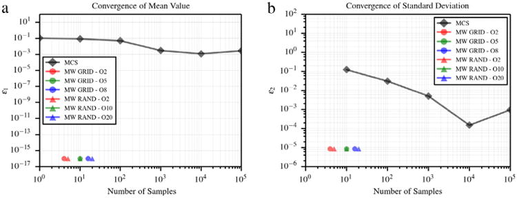
Error in average value (a) and standard deviation (b) for identity map of Gaussian random variable computed using a multi-wavelet expansion with orthogonality with respect to the truncated Gaussian distribution.

Fig. 5.

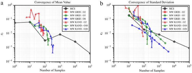
Error in average value (a) and standard deviation (b) for identity map of Gaussian random variable computed using a multi-wavelet expansion with orthogonality with respect to 𝒰(0, 1) and transformation through projections on the cumulative distribution. Note that in (a) the statistics computed using quadrature grids of increasing order are not visible, due to the very small associated error.

6.3. Discontinuous function in two dimensions

We consider the discontinuous function proposed in [30]:

$$u(y_1,y_2)=\{\begin{array}{cc}sin(\pi y_1)sin(\pi y_2)& \text{if}{y}_1\le 0.5,y_2\le 0.5\\ 0& \text{otherwise}\end{array},$$ (49)

where the random variables y₁, y₂ are independent and uniformly distributed on (0, 1)². This function has two line discontinuities along y₁ = 1/2 and y₂ = 1/2, respectively, and thus methods based on global polynomial regression are likely to result in poor approximation. Convergence plots for the mean and standard deviation are shown in Fig. 7. The 2nd-order sparse grid is unable to provide an accurate approximation of ν₂. While areas where u(y₁, y₂) = 0 are correctly approximated, computation of expansion coefficients involving the product of a quadratic basis with a sinusoidal response is not accurate.

Fig. 7.

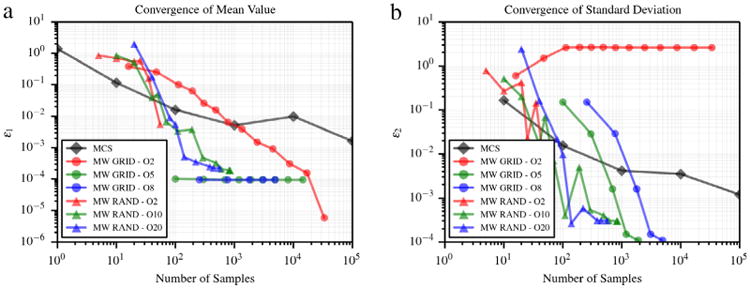
Error in average value (a) and standard deviation (b) for the discontinuous function proposed in [30]

6.4. Non aligned slope discontinuity in two dimensions

Convergence of the proposed formulation is demonstrated, in this section, for an analytical function with slope discontinuity not aligned with the Cartesian axis. This example is proposed in [10] to show the convergence properties of an adaptive hierarchical sparse grid collocation algorithm. Consider the function on (0, 1)² defined as:

$$u(y_1,y_2)=\frac{1}{|0.3-y_1^2-y_2^2|+\delta },$$ (50)

where δ = 10⁻¹. Convergence plots are shown in Fig. 8. The advantages of random sampling (with a minimum number of 10 and 20 samples per element) start to appear both in the computation of the average value and standard deviation. For responses with features not aligned with the adopted Cartesian integration grid, improved approximation results from a combination of random sampling and RVM regression.

Fig. 8.

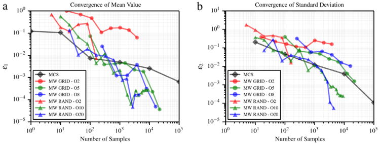
Error in average value (a) and standard deviation (b) for the function with slope discontinuity proposed in [10].

For this and the previous case (a visualization of their stochastic response and parameter space refinement is shown in Fig. 6), we look at both the convergence in terms of the first and second order statistical moments, and the ℓ₁, ℓ₂ and ℓ_∞ error norms evaluated at n_MC = 10³ random points uniformly distributed on Σ_y = (0, 1)². Specifically, the following expressions are used:

Fig. 6.

Representation of the two non-smooth benchmark functions. The first (a) is expressed through the relationship (49) and has been proposed in [30], while the second (b) is expressed using (50) and proposed in [10]. For this latter function, the hypercube partition at refinement iteration 19 is also shown (c).

$$\begin{array}{c}{e}_{\infty }=\underset{i=1,\dots ,n_{MC}}{max}|u^{(i),\ast }(y_1,y_2)-u^{(i)}(y_1,y_2)|,\\ e_1=\frac{1}{n_{MC}}\sum _{i=1}^{n_{MC}}|u^{(i),\ast }(y_1,y_2)-u^{(i)}(y_1,y_2)|,\\ e_2={\left\{\frac{1}{n_{MC}}\sum _{i=1}^{n_{MC}}{[u^{(i),\ast }(y_1,y_2)-u^{(i)}(y_1,y_2)]}^2\right\}}^{1/2},\end{array}$$ (51)

where u^(i),* represents the approximation computed through the proposed multi-resolution regression at the ith check point and the associated exact solution u⁽ⁱ⁾. Monotonic convergence is observed for both quadrature grids and random samples (see Fig. 9), where the former require significant additional samples. This plot further highlights the benefits of the proposed approach with respect to grid collocation.

Fig. 9.

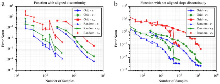
Convergence of error norms e₁, e₂ and e_∞, plotted using 1000 random check points. (a) Convergence for (49), (b) convergence for (50).

6.5. The Kraichnan–Orszag problem

The Kraichnan–Orszag (KO) problem has become a standard benchmarks for adaptive uncertainty propagation algorithms (see, e.g., [10,9]). It consists of a system of three coupled non-linear ODEs derived from the simplified inviscid Navier–Stokes equations [31]. When uncertainty is injected in the initial conditions of the three state variables, the stochastic response is characterized by sharp gradients that rapidly evolve with time. In this section, we adopt a formulation of the KO problem discussed in [9], expressed through the following system:

$$\begin{array}{ccc}\frac{d{u}_1}{dt}=u_1{u}_3,& \frac{d{u}_2}{dt}=u_2{u}_3,& \frac{d{u}_3}{dt}=u_1^2+u_2^2.\end{array}$$ (52)

Note that when the set of initial conditions is selected such that the planes u₁ = 0 and u₂ = 0 are consistently crossed, the accuracy of the global polynomial approximations (at the stochastic level) deteriorates rapidly in time [9].

6.6. One dimensional Kraichnan–Orszag problem

We assume initial conditions for (52) to be random and specified as

$$\begin{array}{ccc}{u}_1(t=0)=1,& u_2(t=0)=0.2y-0.1,& u_3(t=0)=0,\end{array}$$ (53)

where y is uniformly distributed on (0, 1). Fig. 12(a) illustrates the adaptive reconstruction of u₁(y) for an increasing number of elements with samples generated from a double Clenshaw–Curtis integration rule, while Fig. 10 shows the convergence of the first two estimated statistical moments of u₁(y). Convergence plots are shown in Fig. 10. While lower grid orders or number of samples provide inaccurate estimates of the standard deviation, significant improvements over Monte Carlo Sampling are obtained by adding more samples. We note that the stochastic response is characterized by sharp local features (Fig. 12(a)). Under these conditions, the efficiency of collocation grids is maximized, resulting in similar sample requirements as random sampling.

Fig. 12.

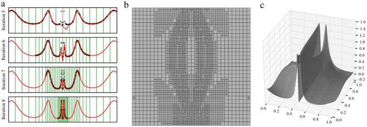
Iterative refinement of (0, 1) and progressive approximation of the stochastic response u₁(y, t) at t = 30 s for the one-dimensional KO problem (a). Refinement of (0, 1)² (b) and reconstructed response (c) for the two-dimensional KO problem.

Fig. 10.

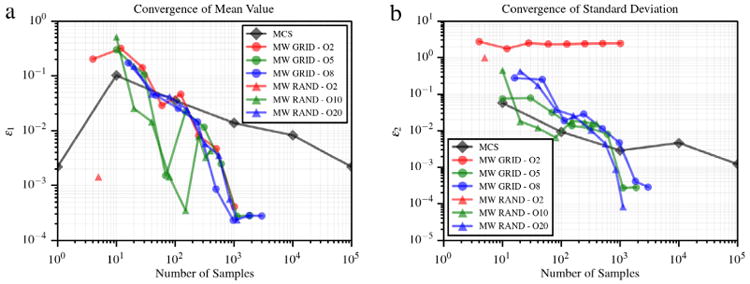
Convergence in average value (a) and standard deviation (b) for the 1D KO problem.

6.7. Two dimensional Kraichnan–Orszag problem

The initial conditions of the Kraichnan–Orszag problem are assumed to be uncertain and functions of two random variables

$$\begin{array}{ccc}{u}_1(t=0)=1,& u_2(t=0)=0.2y_1-0.1,& u_3(t=0)=2y_2-1,\end{array}$$ (54)

where y₁ and y₂ are independent and uniformly distributed on (0, 1). A two dimensional multi-wavelet approximation of u₁ at t = 10 s is generated with m = 2. Fig. 11(a) shows the convergence of average value and standard deviation of u₁ using MCS, and a multi-wavelet approximation evaluated on sparse grid and random adaptive sampling. Finally, Fig. 12(b) and (c) show the obtained partition of (0, 1)² using tensor grids at refinement iteration 17. Convergence plots are shown in Fig. 11. The proposed approach with random sampling outperforms both grid collocation and MCS.

Fig. 11.

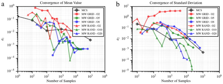
Convergence in average value (a) and standard deviation (b) for the 2D KO problem.

6.8. Three dimensional Kraichnan–Orszag problem

The initial conditions of the three-dimensional Kraichnan–Orszag problem are

$$\begin{array}{ccc}{u}_1(t=0)=0.2y_1-1.0,& u_2(t=0)=0.2y_2-0.1,& u_3(t=0)=0.2y_3-1.0,\end{array}$$ (55)

where we assume that y₁, y₂ and y₃ are independent and uniformly distributed on (0, 1). The multi-wavelet approximation at t = 10 s is constructed for u₁ using m = 2. The convergence plots for the standard deviation are shown in Fig. 13. Unlike the prior results, random sampling outperforms quadrature grids but shows a convergence similar to Monte Carlo Sampling, due to the complex features of the stochastic response [10]. While we do not expect, in practice, stochastic responses with features as complicated as this benchmark problem, this case illustrates that the algorithm can compute converging statistics in such cases.

Fig. 13.

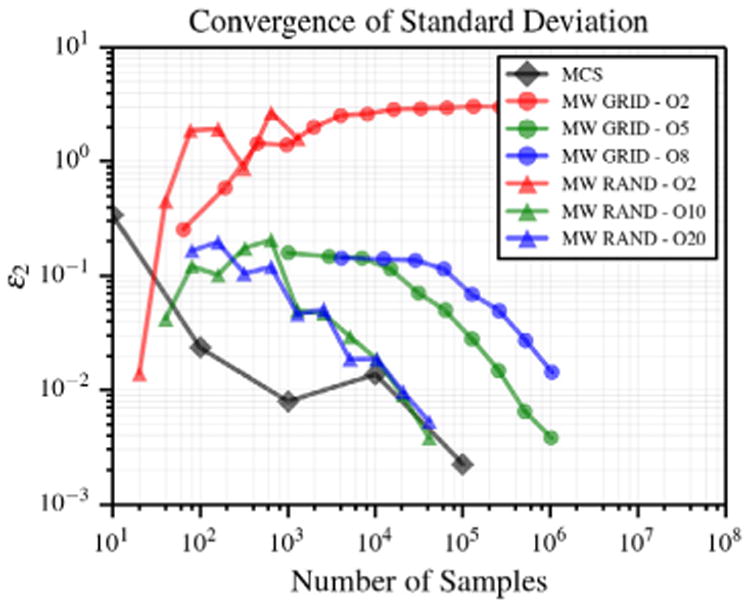
Convergence in standard deviation for the 3D KO problem.

7. Application: Forward propagation of local hemodynamic statistics

7.1. Motivation

We discuss the application of the proposed framework to a problem in uncertainty propagation for cardiovascular blood flow simulation. Specifically, we are interested in determining both mean values and variability of local hemodynamic quantities in the coronary arteries, in patients following coronary artery bypass graft (CABG) surgery.

To do so, we employ a multi-scale modeling strategy that includes a three-dimensional model of the patient's aorta, aortic branches and coronary arteries, receiving pressure/velocity boundary conditions from a lumped parameter description of the peripheral circulation. This lumped parameter or zero-dimensional (0D) boundary model is analogous to an electrical circuit and parameterized through a set of resistances (viscous resistance of the blood), capacitances (vessels compliance), inductances (blood inertia) and other parameters regulating the heart function. An three-dimensional anatomical model was constructed using the Simvascular software package [32], starting from a set of patient-specific CT images. A schematic representation of a typical multi-scale model for coronary artery disease is depicted in Fig. 14.

Fig. 14.

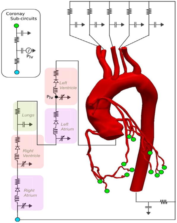
Schematic representation of a multi-scale model for coronary artery bypass surgery from [33]. The anatomical model contains the aortic arch, thoracic aortic branches, coronary arteries and bypass grafts. The boundary conditions are provided by a lumped parameter model that mimics the heart and peripheral circulation.

It is evident how a multiplicity of pressure/velocity boundary conditions (or alternatively of 0D model parameters) are able to generate multi-scale model outputs compatible with non-invasively acquired clinical data, especially if these data are affected by uncertainty. We are therefore interested in first determining the distributions of boundary conditions by performing data assimilation, i.e., by estimating the 0D model parameters using adaptive Markov chain Monte Carlo (MCMC). Due to the number of model evaluations typically required to produce independent samples from a stationary posterior distribution in MCMC, a condensed resistive representation of the three-dimensional model is also computed, leading to a dramatic reduction in the overall computational cost (from several hours to a fraction of a second, see [33], for a single model solution). The proposed multi-resolution approach to uncertainty propagation is employed to propagate the distributions of assimilated boundary conditions through a full multi-scale model, therefore quantifying the variability in local hemodynamic indicators of interest.

Finally, we address the reasons why the proposed approach should be preferred to Monte Carlo Simulation for cardiovascular applications. The primary factors in the choice of method are the moderate dimensionality, the non-smoothness of the stochastic response (likely limited to a small subsets of dimensions), and the high computational cost needed to produce each multi-scale model evaluation. These conditions arise particularly when studying the effect of combined uncertainty sources, e.g., clinical data, model geometry and vessel wall material properties. Specifically, changes in the model geometry for configurations characterized by competing flow (e.g., total cavopulmonary connection in Fontan completion surgery [34]) are likely to produce a non-smooth variation in the outputs. Under these conditions and from the results of the numerical experiments in Section 6, the proposed approach is likely to result in computational savings with respect to MCS due to the smaller number of model evaluations needed to capture the statistics of interest.

7.2. Clinical targets selection and parameter identifiability study

In this section we provide details on the preliminary steps needed to produce random input samples for the uncertainty propagation task. Specifically, we discuss clinical target selection for data assimilation and preliminary identifiability analysis. Please refer to [33] for further details. Targets were acquired using routine clinical measurements, population average values, echocardiography data, and complemented with literature data on coronary flow. Diastolic, systolic and mean aortic pressures were estimated from the patient's cuff pressures during echocardiogram. Other patient-specific measurements from echocardiography included stroke volume, ejection fraction, ratio of early to late flows into the left ventricle, valve opening times relative to the heart cycle duration, systolic pressure difference between the right ventricle and right atrium measured from tricuspid valve regurgitation, and the mean right atrial pressure estimated from the diameter and degree of inspiratory collapse of the inferior vena cava [33].

Additional data from literature was used to improve parameter identifiability. In this regard, a mean pulmonary pressure of 14.0 mmHg was considered together with 4% of the cardiac output entering the coronaries. Representative left and right coronary waveforms from Doppler flow wire measurements [35] were also used to quantify the diastolic to systolic coronary peak flow ratio, the diastolic to systolic coronary blood volume, and the ratio of the flow in the coronary arteries occurring in the first 1/3 and 1/2 of the heart cycle.

Standard deviations for these targets were determined from the literature and personal communication with our clinical collaborators. Measurements derived from tracking the left ventricular wall during echocardiography are characterized by limited uncertainty, whereas higher uncertainties occur in flow measurements from doppler echocardiography.

Identification of both influential and unimportant parameters was performed using a combination of prior experience in manual tuning, analysis of structural identifiability through the Fisher Information Matrix (FIM), and the marginal parameter distributions resulting from Bayesian estimation (where a flat marginal posterior is generally indicative of unimportant parameters). Previous experience with manual tuning allowed us to immediately identify parameters significantly affecting the systemic blood pressure, stroke volume, systemic to coronary flow split, and qualitative shape of the coronary flow waveforms. The left ventricular elastance E_lv affects the stroke volume and mean systemic blood pressure, while the aortic compliance C_ao affects the systemic diastolic to systolic pressure range. The coronary downstream resistance scaling factor R_am,cor has a strong influence on the flow splits, while the coronary capacitances and dP/dt_r (i.e., the intramyocardial pressure time derivative) significantly affect the shape of the coronary waveforms. The downstream systemic resistance scaling factor R_rcr affects both the aortic diastolic to systolic pressure range and the stroke volume.

The Fisher Information Matrix (FIM) rank is a local measure of identifiability, i.e., the ability to uniquely characterize parameter combinations from the available observations [36]. A singular FIM reveals the presence of non-identifiable parameter combinations and an analysis of the eigenvectors associated with the zero eigenvalues (so-called null eigenvectors) can be useful to identify these parameters. In this regard, a null eigenvector with a dominant component along a certain parameter typically suggests this parameter to be unimportant. Thus, we used the FIM to detect all the unimportant parameters until no more trivial null eigenvectors were found.

We then examined the estimated posterior marginal variance as a measure of global identifiability. In particular, we quantified the ability to learn the parameter y_i by comparing the posterior and prior marginal variances using the coefficient θ_i as

$${\theta }_i=1-\sqrt{\frac{{\nu }_2[y_i|\mathbf{d}]}{{\nu }_2[\mathbf{d}]}}$$ (56)

where ν₂[y_i |d] and ν₂[d] are the posterior and prior marginal variances, respectively. Well-learned parameters will have a much smaller variance after being conditioned to the clinical observations (θ → 1), while poorly learned parameters, on the other hand, will have resulting variances that are close to their prior variance (θ → 0). Intuitively, parameters associated with large marginal variances will likely have a limited impact on the model results selected for identification, since these parameters can take on a wide range of values, but produce results with similar posterior.

Prior tuning experience, FIM analysis, Bayesian learning metrics, and qualitative knowledge of expected physiologic coronary waveforms, allowed us to determine a reduced set of 13 parameters (see Table 3). This subset consistently generated excellent agreement between model outputs and clinical targets, and produced flow and pressure waveforms consistent with qualitative expectations [33].

Table 3.

Thirteen identifiable 0D model parameters included as stochastic inputs.

Parameter	Description	Parameter	Description
Erσ	Right ventricular elastance.	Cam,l	Distal capacitance at left coronary outlet.
Elσ	Left ventricular elastance.	Ca,l	Proximal capacitance at left coronary outlet.
Elσp	Scaling factor for left ventricular elastance rate.	Cam,r	Distal capacitance at right coronary outlet.
Cao	Aortic compliance.	Ca,r	Proximal capacitance at right coronary outlet.
Kxp,ra	Passive right atrial curve scaling factor.	Rrcr	Downstream systemic resistance scaling factor.
Kxp,la	Passive left atrial curve scaling factor.	dP/dtr	Intramyocardial pressure time derivative.
Ram	Coronary downstream resistance scaling factor.

An adaptive Markov chain Monte Carlo strategy was used, at this point, to sample from the posterior distribution of these 13 model parameters, constructed using the clinical data and associated uncertainty discussed above.

7.3. Uncertainty propagation results

The availability of samples from the joint posterior distribution of the random inputs, is a prerequisite to performing uncertainty propagation using the proposed approach, with the goal of statistically quantifying the outputs of interest. As a first step, the marginals were determined for the random inputs y (Fig. 15) as well as the coefficients β^(k), k = 1, … , M. We then used 64 sub-samples from the MCMC parameter traces (after removing the realizations produced during burn-in, see [37]) and computed solutions of the full multi-scale model at these realizations using a stabilized finite element solver [38]. Note how the parameter realizations provided by MCMC are roughly 1.5M and it would be impossible to compute a stabilized finite element solution for all the MCMC parameter realizations. Statistics were computed through Monte Carlo averaging and by forward propagation using the proposed multi-resolution approach, using the same number of model solutions (64) for various multi-wavelet orders. Results were very similar to those provided by MCS, as shown in Figs. 16 and 17. Fig. 16 reports the average value and standard deviation for the pressure distribution in one of the seven patients analyzed in [33]. We see that the standard deviation is not negligible in this case, and the proposed approach with a multi-wavelet order of 1 produces the same results as MCS. Fig. 17 represents a typical case where, instead, the variability of wall shear stress-derived quantities is negligible with respect to the associated mean value. We observe that, even in these cases, there is a good agreement between the MCS results and those produced by the proposed approach.

Fig. 15.

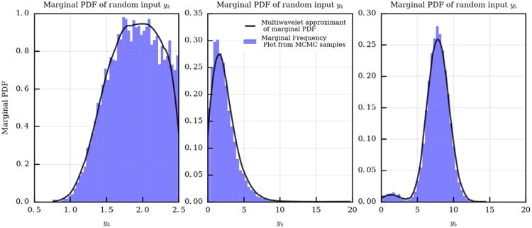
Normalized frequency plots and multiwavelet approximants for the marginal PDF of random inputs y₃, y₄ and y₅.

Fig. 16.

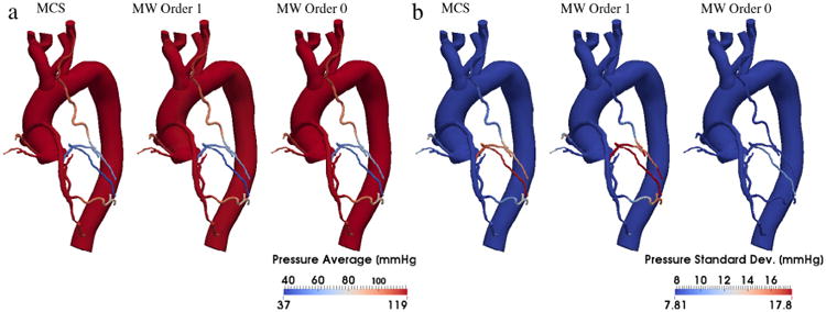
Contour plot representing the estimates of the average pressure (a) and its standard deviation (b) on a three-dimensional multi-scale model of the aorta and coronary circulation. The statistics of the proposed multi-resolution approach are compared to those obtained from Monte Carlo sampling, computed over 64 realizations.

Fig. 17.

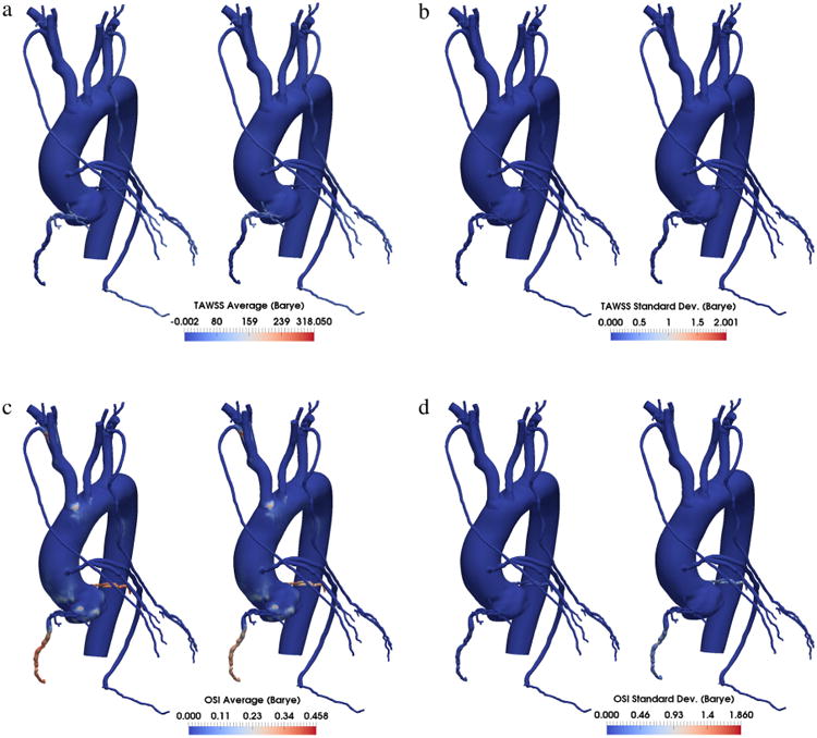
Comparison between average and standard deviation of time averaged wall shear stress (TAWSS) and oscillatory shear index (OSI) computed using Monte Carlo simulation and the proposed multi-resolution approach. The two approaches result in practically the same contours for the quantities of interests.

This confirms the accuracy of the approach when random inputs are not independent, but available through MCMC samples. Moreover, we have shown in the previous sections that the proposed approach outperforms MCS, requiring in most cases a significantly smaller number of model evaluations to accurately compute the output statistics. This suggests that multi-resolution uncertainty propagation has enough flexibility to handle cases where estimated distributions of boundary conditions are combined with assumed geometrical and/or material parameter uncertainties. Future studies will investigate the performance of the proposed approach under these more general settings.

8. Conclusion

We propose a generalized multi-resolution expansion with random inputs characterized by arbitrary probability distributions and random sample locations. The framework has built-in adaptivity metrics based on the natural decomposition of the total regressor variance in multi-scaling and multi-wavelet contributions. A set of ad-hoc multi-resolution bases is constructed orthonormal with respect to an arbitrary distribution function defined on a subset of the input space. This approach, particularized to uniform underlying measures with Legendre multi-scaling, can be used to evaluate the integration constant and the marginal distributions from Markov chain Monte Carlo samples, allowing to perform expectations of arbitrary correlated random inputs. Performance and convergence of the method was demonstrated on several model problems and on a large scale computational model in cardiovascular hemodynamics. For problems in stochastic cardiovascular modeling, especially under a multiplicity of uncertainty sources, the proposed approach is expected to provide a computationally more efficient alternative to Monte Carlo Sampling, leading to accurate statistics with a smaller number of required multi-scale model evaluations.

References

- 1.Wiener N. The homogeneous chaos. Amer J Math. 1938;60:897–936. [Google Scholar]
- 2.Cameron R, Martin W. The orthogonal development of non-linear functionals in series of Fourier-Hermite functionals. Ann of Math. 1947:385–392. [Google Scholar]
- 3.Ghanem R, Spanos P. Stochastic Finite Elements: A Spectral Approach. Courier Corporation; 2003. [Google Scholar]
- 4.Xiu D, Karniadakis G. The Wiener–Askey polynomial chaos for stochastic differential equations. SIAM J Sci Comput. 2002;24:619–644. [Google Scholar]
- 5.Ernst O, Mugler A, Starkloff H, Ullmann E. On the convergence of generalized polynomial chaos expansions. ESAIM Math Model Numer Anal. 2012;46:317–339. [Google Scholar]
- 6.Babuؖka I, Nobile F, Tempone R. A stochastic collocation method for elliptic partial differential equations with random input data. SIAM J Numer Anal. 2007;45:1005–1034. [Google Scholar]
- 7.Nobile F, Tempone R, Webster C. A sparse grid stochastic collocation method for partial differential equations with random input data. SIAM J Numer Anal. 2008;46:2309–2345. [Google Scholar]
- 8.Nobile F, Tempone R, Webster C. An anisotropic sparse grid stochastic collocation method for partial differential equations with random input data. SIAM J Numer Anal. 2008;46:2411–2442. [Google Scholar]
- 9.Wan X, Karniadakis G. An adaptive multi-element generalized polynomial chaos method for stochastic differential equations. J Comput Phys. 2005;209:617–642. [Google Scholar]
- 10.Ma X, Zabaras N. An adaptive hierarchical sparse grid collocation algorithm for the solution of stochastic differential equations. J Comput Phys. 2009;228:3084–3113. [Google Scholar]
- 11.Witteveen J, Iaccarino G. Simplex stochastic collocation with random sampling and extrapolation for nonhypercube probability spaces. SIAM J Sci Comput. 2012;34:A814–A838. [Google Scholar]
- 12.Doostan A, Owhadi H. A non-adapted sparse approximation of PDEs with stochastic inputs. J Comput Phys. 2011;230:3015–3034. [Google Scholar]
- 13.Peng J, Hampton J, Doostan A. A weighted ℓ1-minimization approach for sparse polynomial chaos expansions. J Comput Phys. 2014;267:92–111. [Google Scholar]
- 14.Bilionis I, Zabaras N. Multidimensional adaptive relevance vector machines for uncertainty quantification. SIAM J Sci Comput. 2012;34:B881–B908. [Google Scholar]
- 15.Le Maıtre O, Najm H, Ghanem R, Knio O. Multi-resolution analysis of Wiener-type uncertainty propagation schemes. J Comput Phys. 2004;197:502–531. [Google Scholar]
- 16.Schiavazzi D, Doostan A, Iaccarino G. Sparse multiresolution regression for uncertainty propagation. Int J Uncertain Quantif. 2014;4 [Google Scholar]
- 17.Sankaran S, Marsden A. A stochastic collocation method for uncertainty quantification and propagation in cardiovascular simulations. J Biomech Eng. 2011;133:031001. doi: 10.1115/1.4003259. [DOI] [PubMed] [Google Scholar]
- 18.Sankaran S, Marsden A. The impact of uncertainty on shape optimization of idealized bypass graft models in unsteady flow. Phys Fluids. 2010;22:121902. 1994-present. [Google Scholar]
- 19.Xiu D, Sherwin S. Parametric uncertainty analysis of pulse wave propagation in a model of a human arterial network. J Comput Phys. 2007;226:1385–1407. [Google Scholar]
- 20.Schiavazzi D, Arbia G, Baker C, Hlavacek A, Hsia T, Marsden A, Vignon-Clementel I, et al. Uncertainty quantification in virtual surgery hemodynamics predictions for single ventricle palliation. Int J Numer Methods Biomed Eng. 2015 doi: 10.1002/cnm.2737. [DOI] [PubMed] [Google Scholar]
- 21.Alpert B. A class of bases in L2 for the sparse representation of integral operators. SIAM J Math Anal. 1993;24:246–262. [Google Scholar]
- 22.Soize C, Ghanem R. Physical systems with random uncertainties: chaos representations with arbitrary probability measure. SIAM J Sci Comput. 2004;26:395–410. [Google Scholar]
- 23.Golub G, Welsch J. Calculation of Gauss quadrature rules. Math Comp. 1969;23:221–230. [Google Scholar]
- 24.Clenshaw C, Curtis A. A method for numerical integration on an automatic computer. Numer Math. 1960;2:197–205. [Google Scholar]
- 25.Blatman G, Sudret B. Adaptive sparse polynomial chaos expansion based on least angle regression. J Comput Phys. 2011;230:2345–2367. [Google Scholar]
- 26.Tipping M. Sparse Bayesian learning and the relevance vector machine. J Mach Learn Res. 2001;1:211–244. [Google Scholar]
- 27.Tipping M, Faul A, et al. Fast marginal likelihood maximisation for sparse Bayesian models. Proceedings of the Ninth International Workshop on Artificial Intelligence and Statistics. 2003;1 [Google Scholar]
- 28.Sobol I. Global sensitivity indices for nonlinear mathematical models and their Monte Carlo estimates. Math Comput Simulation. 2001;55:271–280. [Google Scholar]
- 29.Loeve M. Probability Theory II (Graduate Texts in Mathematics) 1994 [Google Scholar]
- 30.Agarwal N, Aluru N. A domain adaptive stochastic collocation approach for analysis of MEMS under uncertainties. J Comput Phys. 2009;228:7662–7688. [Google Scholar]
- 31.Kraichnan R. Direct-interaction approximation for a system of several interacting simple shear waves. Phys Fluids. 1963;6:1603–1609. 1958-1988. [Google Scholar]
- 32.Wilson N, Wang K, Dutton R, Taylor C. Medical Image Computing and Computer-Assisted Intervention–MICCAI 2001. Springer; 2001. A software framework for creating patient specific geometric models from medical imaging data for simulation based medical planning of vascular surgery; pp. 449–456. [Google Scholar]
- 33.Tran J, Schiavazzi D, Bangalore Ramachandra A, Kahn A, Marsden A. Automated tuning for parameter identification and uncertainty quantification in multi-scale coronary simulations. Comput Fluids. 2016 doi: 10.1016/j.compfluid.2016.05.015. in press. [DOI] [PMC free article] [PubMed] [Google Scholar]
- 34.Fontan F, Baudet E. Surgical repair of tricuspid atresia. Thorax. 1971;26:240–248. doi: 10.1136/thx.26.3.240. [DOI] [PMC free article] [PubMed] [Google Scholar]
- 35.Ofli E, Kern M, Vrain J, Donohue T, Bach R, Al-Joundi B, Aguirre F, Castello R, Labovitz A. Differential characterization of blood flow, velocity, and vascular resistance between proximal and distal normal epicardial human coronary arteries: analysis by intracoronary Doppler spectral flow velocity. Am Heart J. 1995;130:37–46. doi: 10.1016/0002-8703(95)90233-3. [DOI] [PubMed] [Google Scholar]
- 36.Rothenberg T. Identification in parametric models. Econometrica. 1971:577–591. [Google Scholar]
- 37.Geyer C. Practical Markov chain Monte Carlo. Statist Sci. 1992:473–483. [Google Scholar]
- 38.Whiting C, Jansen K. A stabilized finite element method for the incompressible Navier–Stokes equations using a hierarchical basis. Int J Numer Methods Fluids. 2001;35:93–116. [Google Scholar]