Abstract
The MDplot package provides plotting functions to allow for automated visualisation of molecular dynamics simulation output. It is especially useful in cases where the plot generation is rather tedious due to complex file formats or when a large number of plots are generated. The graphs that are supported range from those which are standard, such as RMsD/RMsF (root-mean-square deviation and root-mean-square fluctuation, respectively) to less standard, such as thermodynamic integration analysis and hydrogen bond monitoring over time. All told, they address many commonly used analyses. In this article, we set out the MDplot package′s functions, give examples of the function calls, and show the associated plots. Plotting and data parsing is separated in all cases, i.e. the respective functions can be used independently. Thus, data manipulation and the integration of additional file formats is fairly easy. Currently, the loading functions support GROMOS, GROMACS, and AMBER file formats. Moreover, we also provide a Bash interface that allows simple embedding of MDplot into Bash scripts as the final analysis step.
Availability
The package can be obtained in the latest major version from CRAN (https://cran.r-project.org/package=MDplot) or in the most recent version from the project′s GitHub page at https://github.com/MDplot/MDplot, where feedback is also most welcome. MDplot is published under the GPL-3 license.
Introduction
The amount of data produced by molecular dynamics (MD) engines (such as GROMOS (Schmid et al., 2012; Eichenberger et al., 2011), GROMACS (Pronk et al., 2013), NAMD (Phillips et al., 2005), AMBER (Cornell et al., 1995), and CHARMM (Brooks et al., 2009)) has been constantly increasing over recent years. This is mainly due to more powerful and cheaper hardware. As a result of this, both the lengths and sheer number of MD simulations (i.e. trajectories) have increased enormously. Even large sets of simulations (e.g., in the context of drug design) are attainable nowadays; thus suggesting that the processing of the resulting information is undertaken automatically.
In this respect, automated yet flexible visualisation of molecular dynamics data would be highly advantageous: both in order to avoid repetitive tasks for the user and to yield the ultimately desired result instantly (see Figure 1). Moreover, generating some of the graphs can be cumbersome. An example would be the plotting of a time series of a clustering program or hydrogen bonds. Therefore, these cases are predestined to be handled by a plotting library. There have been attempts made in that direction, for example the package bio3d (Grant et al., 2006; Skjærven et al., 2014) (which allows the trajectories to be processed in terms of principle component analysis (PCA), RMSD and RMSF calculations), MDtraj (McGibbon et al., 2015), or Rknots (Comoglio and Rinaldi, 2012). However, to the best of our knowledge, there is currently no R package available that offers the wide range of plotting functions and engine-support that is provided by MDplot. R is the natural choice for this undertaking because of both its power in data handling and its vast plotting abilities.
Figure 1.
Shows the overall workflow typically applied in molecular dynamics simulations beginning with a single PDB (Berman et al., 2000) structure as the input for the simulation and ending with the graphical representation of the data obtained. For large amounts of data, generating figures might become a tedious, highly repetitive task.
In the following sections we outline all of the plotting functions that are currently supported. For each function, examples of the function calls based on the test data included in the package, the resulting plots, the return values, and a table of arguments are detailed. The respective code samples use the loading functions (reported below) to parse the input files located in folder ′extdata′, which allows immediate testing and provides format information to users. Currently, the package supports GROMOS, GROMACS, and AMBER file formats as input.1 However, extensions in both format support and plotting functionalities are planned.
Plotting functions
The package currently offers 14 distinct plotting functions (Table 1), which cover many of the graphs that are commonly required. Although the focus of the package relies on the visualisation of data, in addition to this values are calculated to characterise the underlying data when appropriate. For example, TIcurve() calculates the thermodynamic integration free-energy values including error estimates and the hysteresis between the integration curves. In many cases, the plotting functions return useful information on the data used, e.g., range, mean and standard deviation of curves.
To provide simple access to these functions, they may be called from within a Bash script. Examples are provided at the end of the manuscript.
Table 1.
Lists all of the currently available plotting functions that have been implemented in MDplot. Most functions accept a boolean parameter (barePlot), that indicates printing of the plotting area only, i.e. stripped from any additional features such as axis labels.
| Plot function | Description |
|---|---|
| clusters() | Summary of clustering over trajectories (RMSD based). |
| clusters_ts() | Time series of cluster populations (RMSD based). |
| dssp() | Secondary structure annotation plot (DSSP based). |
| dssp_ts() | Time series of secondary structure elements (DSSP based). |
| hbond() | Hydrogen bonds summary plot. |
| hbond_ts() | Time series of hydrogen bonds. |
| noe() | Nuclear-Overhauser-effect violation plot. |
| ramachandran() | Dihedral angle plot. |
| rmsd() | Root-mean-square deviation plot. |
| rmsd_average() | Average root-mean-square deviation plot. |
| rmsf() | Root-mean-square fluctuation plot. |
| TIcurve() | Thermodynamic integration curves. |
| timeseries() | General time series plot. |
| xrmsd() | Cross-RMSD plot (heat-map of RMSD values). |
The clusters() function
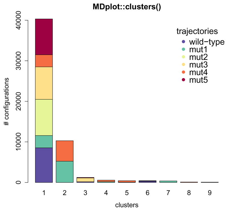
Molecular dynamics simulation trajectories can be considered to be a set of atom configurations along the time axis. Clustering is a method, that can be applied in order to extract common structural features from these. The configurations are classified and grouped together based on the root-mean-square deviation (RMSD). These subsets of configurations around the cluster′s central member structure and their relative occurrences allow for comparisons between different and within individual simulations. clusters() allows to plot a summary of all of the (selected) clusters over a set of trajectories (Figure 2).
Figure 2.
The clusters are plotted along the x-axis and the number of configurations for each trajectory for every cluster on the y-axis. The number of clusters is limited in this example to nine with the clustersNumber argument, which can be useful to omit scarcely populated clusters.
clusters(load_clusters("inst/extdata/clusters_example.txt.gz",
                       names=c("wild-type","mut1","mut2",
                               "mut3","mut4","mut5")),
         clustersNumber=9,main="MDplot::clusters()",ylab="# configurations")
Return value: Returns an n × m-matrix with n being the number of input trajectories and m the number of different clusters. Each element in the matrix holds the number of snapshots, in which the respective cluster occurred in the respective trajectory.
Table 2.
Arguments of the clusters() function.
| Argument name | Default value | Description |
|---|---|---|
| clusters | none | Matrix with clusters: trajectories are given in row-wise, clusters in column-wise fashion as provided by load_clusters(), the associated loading function. |
| clustersNumber | NA | When specified, only these first clusters are shown. |
| legendTitle | “trajectories” | The title of the legend. |
| barePlot | FALSE | A Boolean indicating whether the plot is to be made without any additional information or not. |
| … | none | Additional arguments. |
The clusters_ts() function
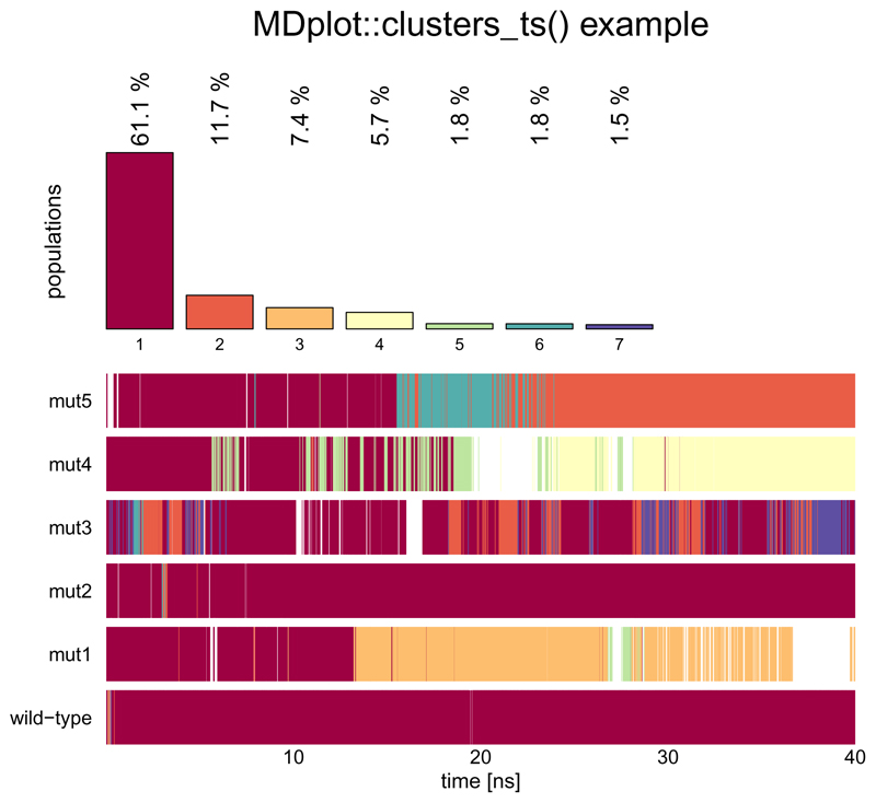
In structural clustering, it is often instructive to have a look at the development over time rather than the overall summary. This functionality is provided by clusters_ts(). In the top sub-plot the overall distribution is given, while the time series is shown at the bottom. The clusters are sorted beginning with the most populated one, in descending order. Selections can be made and clusters that are not selected do also not appear in the time series plot (white areas). The time axis may be shown in nanoseconds (see Figure 3 for an example).
Figure 3.
The plot shows a selection of the seven most populated clusters of six trajectories. Regions that do not belong to one of the first seven clusters are shown in white.
clusters_ts(load_clusters_ts("inst/extdata/clusters_ts_example.txt.gz",
                             lengths=c(4000,4000,4000,4000,4000,4000),
                             names=c("wild-type","mut1","mut2",
                                     "mut3","mut4","mut5")),
            clustersNumber=7,main="MDplot::clusters_ts() example",
            timeUnit="ns",snapshotsPerTimeInt=100)
Return value: Returns a summary (n + 1) × m-matrix with n being the number of input trajectories and m the number of different clusters (which have been plotted). Each element in the matrix holds the number of snapshots, in which the respective cluster occurred in the respective trajectory. In addition, the first line is the overall summary counted over all trajectories.
Table 3.
Arguments of the clusters_ts() function.
| Argument name | Default value | Description |
|---|---|---|
| clustersDataTS | none | List of cluster information as provided by load_clusters_ts(), the associated loading function. |
| clustersNumber | NA | An integer specifying the number of clusters that is to be plotted. |
| selectTraj | NA | Vector of indices of trajectories that are plotted (as given in the input file). |
| selectTime | NA | Range of time in snapshots. |
| timeUnit | NA | Abbreviation of time unit. |
| snapshotsPerTimeInt | 1000 | Number of snapshots per time unit. |
| … | none | Additional arguments. |
The dssp() function
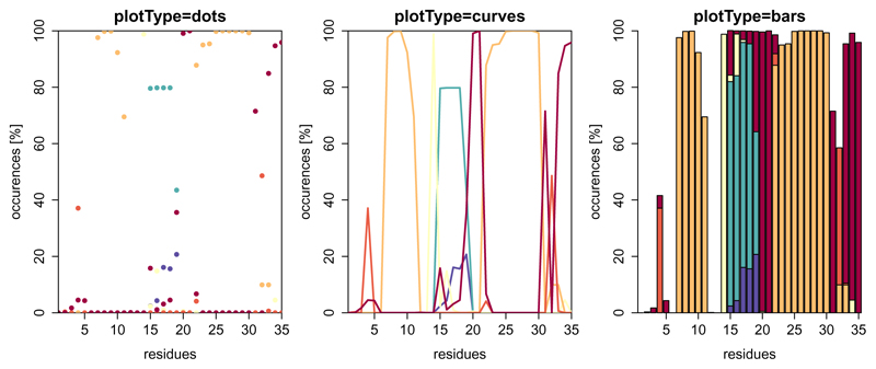
In terms of proteins the secondary structure can be annotated by the widely used program DSSP (Definition of Secondary Structure of Proteins) (Kabsch and Sander, 1983). This algorithm uses the backbone hydrogen bond pattern in order to assign secondary structure elements such as α-helices, β-strands, and turns to protein sequences. The plotting function dssp() has three different visualisation methods and plots the overall result over the trajectory and over the residues. The user can specify selections of residues and which elements should be taken into consideration (Figure 4).
Figure 4.
Example of dssp() with plotType set to ”dots” (default), ”curves” or ”bars”. Note that the fractions do not necessarily sum up to a hundred percent, because some residues might not be in defined secondary structure elements all the time. In this figure, there is no legend plotted due to space limitations (see Figure 5 for a colour-code explanation).
layout(matrix(1:3, nrow=1), widths=c(0.33,0.33,0.33))
dssp(load_dssp("inst/extdata/dssp_example.txt.gz"),
     main="plotType=dots",showResidues=c(1,35))
dssp(load_dssp("inst/extdata/dssp_example.txt.gz"),
     main="plotType=curves",plotType="curves",showResidues=c(1,35))
dssp(load_dssp("inst/extdata/dssp_example.txt.gz"),
     main="plotType=bars",plotType="bars",showResidues=c(1,35))
Return value: Returns a matrix, where the first column is the residue-number and the remaining ones denote secondary structure classes. Residues are given row-wise and values range from 0 to 100 percent.
Table 4.
Arguments of the dssp() function.
| Argument name | Default value | Description |
|---|---|---|
| dsspData | none | Table containing information on the secondary structure elements. Can be generated by function load_dssp(). |
| printLegend | FALSE | If TRUE, a legend is printed on the right hand side of the plot. |
| useOwnLegend | FALSE | If FALSE, the names of the secondary structure elements are considered to be in default order. |
| elementNames | NA | Vector of names for the secondary structure elements. |
| colours | NA | A vector of colours that can be specified to replace the default ones. |
| showValues | NA | A vector of boundaries for the values. |
| showResidues | NA | A vector of boundaries for the residues. |
| plotType | “dots” | Either “dots”, “curves”, or “bars“. |
| selectedElements | NA | A vector of names of the elements selected. |
| barePlot | FALSE | Boolean, indicating whether the plot is to be made without any additional information. |
| … | none | Additional arguments. |
The dssp_ts() function
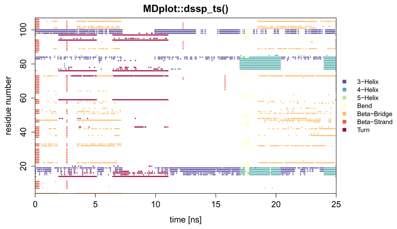
The secondary structure information as described for the function dssp() can also be visualised along the time axis using function dssp_ts() (Figure 5). The time can be annotated in snapshots or time units (e.g., nanoseconds).
Figure 5.
Example showing all of the defined secondary structure elements per residue over time. Note, that for this example plot a sparse data set was used to reduce the size of the data file (hence the large white areas in the middle).
dssp_ts(load_dssp_ts("inst/extdata/dssp_ts_example"),printLegend=TRUE,
        main="MDplot::dssp_ts()",timeUnit="ns",
        snapshotsPerTime=1000)
Table 5.
Arguments of the dssp_ts() function.
| Argument name | Default value | Description |
|---|---|---|
| tsData | none | List of lists, which are composed of a name (string) and a values table (x … snapshots, y … residues). Can be generated by load_dssp_ts(). |
| printLegend | TRUE | If TRUE, a legend is printed on the right hand side of the plot. |
| timeBoundaries | NA | A vector of boundaries for the time in snapshots. |
| residueBoundaries | NA | A vector of boundaries for the residues. |
| timeUnit | NA | If set, the snapshots are transformed into the respective time (depending on parameter snapshotsPerTime). |
| snapshotsPerTimeInt | 1000 | Number of snapshots per respective timeUnit. |
| barePlot | FALSE | A Boolean indicating whether the plot is to be made without any additional information. |
| … | none | Additional arguments. |
The hbond() function
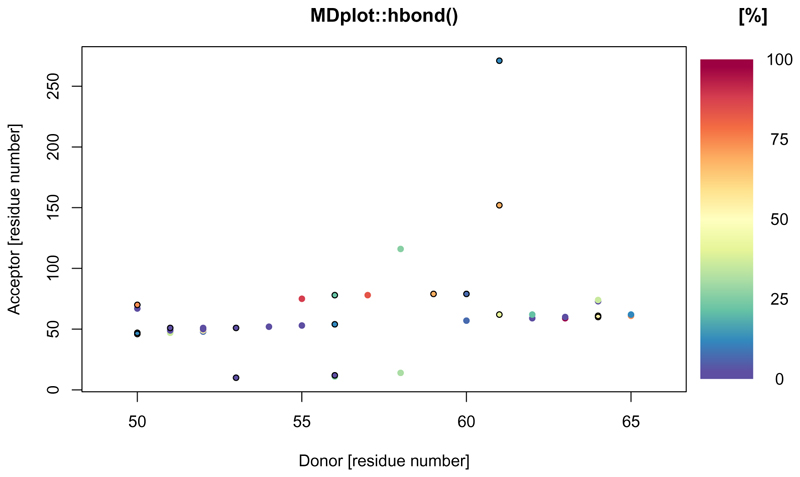
In the context of biomolecules, hydrogen bonds are of particular importance. These bonds take place between a donor, a hydrogen, and an acceptor atom. This function plots the summary output of hydrogen bond calculations and allows selection of donor and acceptor residues. occurrence over the whole trajectory is indicated by a colour scale. Note, that in case multiple hydrogen bond interactions between two particular residues take place (conveyed by different sets of atoms), the interaction with prevalence will be used for colour-coding (and by default, this interaction is marked with a black circle, see below). An example is given in Figure 6.
Figure 6.
The acceptor residues are plotted on the x-axis whilst the donors are shown on the y-axis. The different colours indicate the occurrences throughout the whole trajectory.
hbond(load_hbond("inst/extdata/hbond_example.txt.gz"),
      main="MDplot::hbond()", donorRange=c(0, 65))
Return value: Returns a table containing the information used for plotting in columns as follows:
resDonor Residue number (donor).
resAcceptor Residue number (acceptor).
percentage Percentage, that has been used for colour-coding.
numberInteractions Number of hydrogen bond interactions taking place between the specified donor and acceptor residues.
Table 6.
Arguments of the hbond() function.
| Argument name | Default value | Description |
|---|---|---|
| hbonds | none | Table containing the hydrogen bond information in columns "hbondID", "resDonor", "resDonorName", "resAcceptor", "resAcceptorName", "atom-Donor", "atomDonorName", "atomH", "atomAcceptor", "atomAcceptorName", "percentage" (automatically generated by function load_hbond()). |
| plotMethod | ”residue-wise” | Allows to set the detail of hydrogen bond information displayed. options are: ”residue-wise”. |
| acceptorRange | NA | A vector specifying the range of acceptor residues. |
| donorRange | NA | A vector specifying the range of donor residues. |
| printLegend | TRUE | A Boolean enabling the legend. |
| showMultipleInteractions | TRUE | If TRUE, this option causes multiple interactions between the same residues as being represented by a black circle around the coloured dot. |
| barePlot | FALSE | A Boolean indicating whether the plot is to be made without any additional information. |
| … | none | Additional arguments. |
The hbond_ts() function
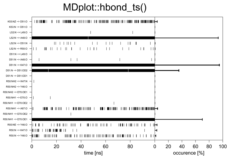
The time series of hydrogen bond occurrences can be visualised using the function hbond_ts(), which plots them either according to their identifiers or in a human readable form in three- or one-letter code (the participating atoms can be shown as well) on the y-axis and the time on the x-axis. If the GROMOS input format is used, this function requires two different files: the summary of the hbond program and the time series file. The occurrence of a hydrogen bond is represented by a black bar and the occurrence summary can be added on the right hand side as a sub-plot (Figure 7). In addition to the time series file, depending on the MD engine format used, an additional summary file might also be necessary (see the documentation of the function load_hbond_ts() for further information).
Figure 7.
Example figure generated by hbond_ts() for both an identifier and acceptor residues′ selection. The labels for the hydrogen bonds may be printed as identifiers or with names composed of residue names (in single- or three-letter code) and those of the participating atoms.
hbond_ts(timeseries=load_hbond_ts("inst/extdata/hbond_ts_example.txt.gz"),
         summary=load_hbond("inst/extdata/hbond_example.txt.gz"),
         main="MDplot::hbond_ts()",acceptorRange=c(22,75),
         hbondIndices=list(c(0,24)),plotOccurences=TRUE,timeUnit="ns",
         snapshotsPerTimeInt=100,printNames=TRUE,namesToSingle=TRUE,
         printAtoms=TRUE)
Return value: Returns an n × 2-matrix, with the first column being the list of hydrogen bond identifiers plotted and the second one the occurrence (in percent) over the selected time range.
Table 7.
Arguments of the hbond_ts() function.
| Argument name | Default value | Description |
|---|---|---|
| timeseries | none | Table containing the time series information (e.g., produced by load_hbond_ts()). |
| summary | none | Table containing the summary information (e.g., produced by load_hbond()). |
| acceptorRange | NA | A vector of acceptor residues. |
| donorRange | NA | A vector of donor residues. |
| plotOccurences | FALSE | Specifies whether the overall summary should be plotted on the right hand side. |
| scalingFactorPlot | NA | Used to manually set the scaling factor (if necessary). |
| printNames | FALSE | Enables human readable names rather than the hydrogen bond identifiers. |
| namesToSingle | FALSE | If printNames is TRUE, this flag instructs one-letter codes instead of three-letter ones. |
| printAtoms | FALSE | Enables atom names in hydrogen bond identification on the y-axis. |
| timeUnit | NA | Specifies the time unit on the x-axis. |
| snapshotsPerTimeInt | 1000 | Specifies how many snapshots make up one time unit (see above). |
| timeRange | NA | A vector specifying a certain time range. |
| hbondIndices | NA | A list containing vectors to select hydrogen bonds by their identifiers. |
| barePlot | FALSE | A Boolean indicating whether the plot is to be made without any additional information. |
| … | none | Additional arguments. |
The noe() function
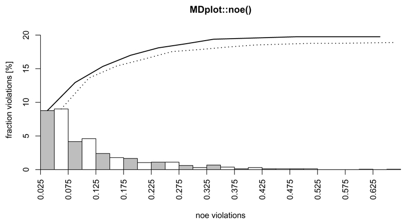
The nuclear-overhauser-effect is one of the most important measures of structure validity in the context of molecular dynamics simulations. These interactions are transmitted through space and arise from spin-spin coupling, which can be measured by nuclear magnetic resonance (NMR) spectroscopy. These measurements provide pivotal distance restrains which should be matched on average during molecular dynamics simulations of the same system and can hence be used for parameter validation. The plotting function noe() allows to visualise the number of distance restrain violations and their respective spatial deviation. As shown in Figure 8, multiple replicates or different protein systems are supported simultaneously. Note that negative violations are not considered.
Figure 8.
Example plot showing two different replicates of a protein simulation (they share the same molecule, but have different initial velocities). Note, that the maximum value (x-axis) over all replicates is used for the plot. The sum over all violations from left to right is shown by an additional curve on top. The number of violations may be given as fractions (in %), as shown above, or absolute numbers (flag printPercentages either TRUE or FALSE).
noe(load_noe(files=c("inst/extdata/noe_example_1.txt.gz",
                     "inst/extdata/noe_example_2.txt.gz")),
    main="MDplot::noe()")
Return value: Returns a matrix, in which the first column holds the bin boundaries used and the following columns represent either the percentage or absolute numbers of the violations per bin, depending on the specification.
Table 8.
Arguments of the noe() function.
| Argument name | Default value | Description |
|---|---|---|
| noeData | none | Input matrix. Generated by function load_noe(). |
| printPercentages | TRUE | If TRUE, the violations will be reported in a relative manner (percent) rather than absolute numbers. |
| colours | NA | Vector of colours to be used for the bars. |
| lineTypes | NA | If plotSumCurves is TRUE, this vector might be used to specify the types of curves plotted. |
| names | NA | Vector to name the input columns (legend). |
| plotSumCurves | TRUE | If TRUE, the violations are summed up from left to right to show the overall behaviour. |
| maxYAxis | NA | Can be used to manually set the y-axis of the plot. |
| printLegend | FALSE | A Boolean indicating if legend is to be plotted. |
| … | none | Additional arguments. |
The ramachandran() function
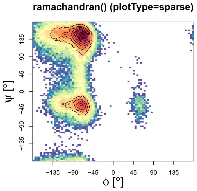
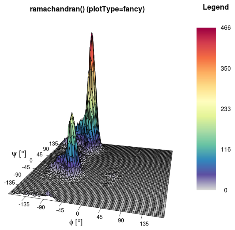
This graph type (Ramachandran et al., 1963) is often used to show the sampling of the ϕ/ψ protein backbone dihedral angles in order to assign propensities of secondary structure elements to the protein of interest (so-called Ramachandran plots). These plots can provide crucial insight into energy barriers arising as required, for example, in the context of parameter validation (Margreitter and Oostenbrink, 2016). The function ramachandran() offers a 2D (Figure 9) and 3D (Figure 10) variant with the former offering the possibility to print user-defined secondary structure regions as well. The number of bins for the two axes and the colours used for the legend can be specified by the user.
Figure 9.
Two-dimensional plot version ”sparse” of the ramachandran() function with enabled contour plotting. The number of bins can be specified for both dimensions independently.
Figure 10.
Three-dimensional example of the ramachandran() function. In addition to the colour, the height (z-axis) also represents the number of dihedrals per bin.
ramachandran(load_ramachandran("inst/extdata/ramachandran_example.txt.gz"),
             heatFun="log",plotType="sparse",xBins=90,yBins=90,
             main="ramachandran() (plotType=sparse)",
             plotContour=TRUE)
ramachandran(load_ramachandran("inst/extdata/ramachandran_example.txt.gz"),
             heatFun="norm",plotType="fancy",xBins=90,yBins=90,
             main="ramachandran() (plotType=fancy)",
             printLegend=TRUE)
Return value: Returns a list of binned dihedral angle occurrences.
Table 9.
Arguments of the ramachandran() function.
| Argument name | Default value | Description |
|---|---|---|
| dihedrals | none | Matrix with angles (two columns). Generated by function load_ramachandran(). |
| xBins | 150 | Number of bins used to plot (x-axis). |
| yBins | 150 | Number of bins used to plot (y-axis). |
| heatFun | “norm” | Function selector for calculation of the colour. The possibilities are either: “norm” for linear calculation or “log” for logarithmic calculation. |
| structureAreas | c() | List of areas, which are plotted as black lines. |
| plotType | “sparse” | Type of plot to be used, either “sparse” (default, using function hist2d()), “comic” (own binning, supports very few datapoints), or “fancy” (3D, using function persp()). |
| printLegend | FALSE | A Boolean specifying whether a heat legend is to be plotted or not. |
| plotContour | FALSE | A Boolean specifying whether a contour should be added or not. |
| barePlot | FALSE | A Boolean indicating whether the plot is to be made without any additional information. |
| … | none | Additional arguments. |
The rmsd() function
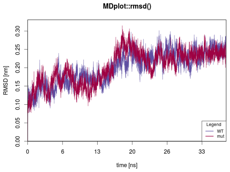
The atom-positional root-mean-square deviation (RMSD) is one of the most commonly used plot types in the field of biophysical simulations. In the context of atom configurations, it is a measure for the positional divergence of one or multiple atoms. The input requires a list of alternating vectors of time indices and RMSD values. Multiple data sets can be plotted, given in separate input files. Figure 11 shows an example for two trajectories.
Figure 11.
This plot shows the RMSD curves for two different trajectories. The time is given in nanoseconds, which requires a properly set factor parameter.
rmsd(load_rmsd(c("inst/extdata/rmsd_example_1.txt.gz",
                 "inst/extdata/rmsd_example_2.txt.gz")),
     printLegend=TRUE,names=c("WT","mut"),main="MDplot::rmsd()")
Return value: Returns a list of lists, where each sub-list represents a RMSD curve and contains the components:
minValue The minimum value over the whole time range.
maxValue The maximum value over the whole time range.
meanValue The mean value calculated over the whole time range.
sd The standard deviation calculated over the whole time range.
Table 10.
Arguments of the rmsd() function.
| Argument name | Default value | Description |
|---|---|---|
| rmsdData | none | List of (alternating) indices and RMSD value vectors, as produced by load_rmsd(). |
| printLegend | TRUE | A Boolean which triggers the plotting of the legend. |
| factor | 1000 | A number specifying how many snapshots are within one timeUnit. |
| timeUnit | “ns” | Specifies the time unit. |
| rmsdUnit | “nm” | Specifies the RMSD unit. |
| colours | NA | A vector of colours used for plotting. |
| names | NA | A vector holding the names of the trajectories. |
| legendPosition | “bottomright” | Indicates the position of the legend: either “bottomright", “bottomleft", “topleft", or “topright". |
| barePlot | FALSE | A Boolean indicating whether the plot is to be made without any additional information. |
| … | none | Additional arguments. |
The rmsd_average() function
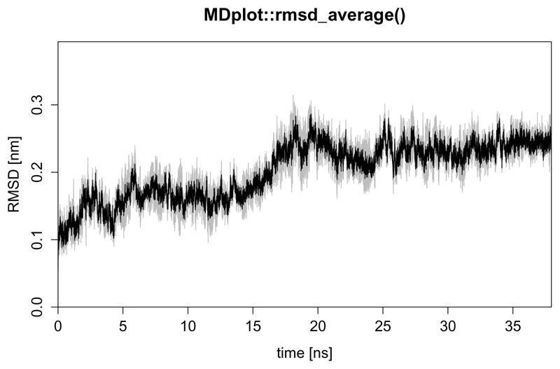
Nowadays, for many molecular systems multiple replicates of simulations are performed in order to enhance the sampling of the phase space. However, since the amount of analysis data grows accordingly, a joint representation of the results may be desirable. For the case of backbone-atom and other RMSD plots, the MDplot package supports average plotting. Instead of plotting every curve individually, the mean and the minimum and maximum values of all trajectories at a given time point is plotted. Thus, the spread of multiple simulations is represented as a ′corridor′ over time.
rmsd_average(rmsdInput=list(load_rmsd("inst/extdata/rmsd_example_1.txt.gz" ),
                            load_rmsd("inst/extdata/rmsd_example_2.txt.gz")),
             maxYAxis=0.375,main="MDplot::rmsd_average()")
Return value: Returns an n × 4-matrix, with the rows representing different snapshots and the columns the respective values as follows:
snapshot Index of the snapshot.
minimum The minimum RMSD value over all input sources at a given time.
mean The mean RMSD value over all input sources at a given time.
maximum The maximum RMSD value over all input sources at a given time.
Table 11.
Arguments of the rmsd_average() function.
| Argument name | Default value | Description |
|---|---|---|
| rmsdInput | none | List of snapshot and RMSD value pairs, as, for example, provided by loading function load_rmsd(). |
| levelFactor | NA | If there are many datapoints, this parameter may be used to use only the levelFactorth datapoints to obtain a clean graph. |
| snapshotsPerTimeInt | 1000 | Number, specifying how many snapshots are comprising one timeUnit. |
| timeUnit | ”ns” | Specifies the time unit. |
| rmsdUnit | ”nm” | Specifies the RMSD unit. |
| maxYAxis | NA | Can be used to manually set the y-axis of the plot. |
| barePlot | FALSE | A Boolean indicating whether the plot is to be made without any additional information. |
| … | none | Additional arguments. |
The rmsf() function
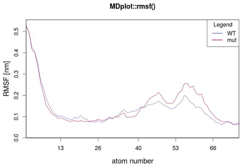
The atom-positional root-mean-square fluctuation (RMSF) represents the degree of positional variation of a given atom over time. The input requires one column with all residues or atoms and a second one holding RMSF values. Figure 13 shows, as an example, the RMSF of the first 75 atoms, calculated for two independent simulations.
Figure 13.
Plot showing two different RMSF curves.
rmsf(load_rmsf(c("inst/extdata/rmsf_example_1.txt.gz",
                 "inst/extdata/rmsf_example_2.txt.gz")),
     printLegend=TRUE,names=c("WT","mut"),range=c(1,75),
     main=“MDplot::rmsf()”)
Return value: A list of vectors, alternately holding atom indices and their respective values.
Table 12.
Arguments of the rmsf() function.
| Argument name | Default value | Description |
|---|---|---|
| rmsfData | none | List of (alternating) atom numbers and RMSF values, as, for example, produced by load_rmsf(). |
| printLegend | TRUE | A Boolean controlling the plotting of the legend. |
| rmsfUnit | "nm" | Specifies the RMSF unit. |
| colours | NA | A vector of colours used for plot. |
| residuewise | FALSE | A Boolean specifying whether atoms or residues are plotted on the x-axis. |
| atomsPerResidue | NA | If residuewise is TRUE, this parameter can be used to specify the number of atoms per residue for plotting. |
| names | NA | A vector of the names of the trajectories. |
| range | NA | Range of atoms. |
| legendPosition | ”topright” | Indicates position of legend: either ”bottomright”, ”bottomleft”, ”topleft”, or ”topright”. |
| barePlot | FALSE | A Boolean indicating whether the plot is to be made without any additional information. |
| … | none | Additional arguments. |
The TIcurve() function
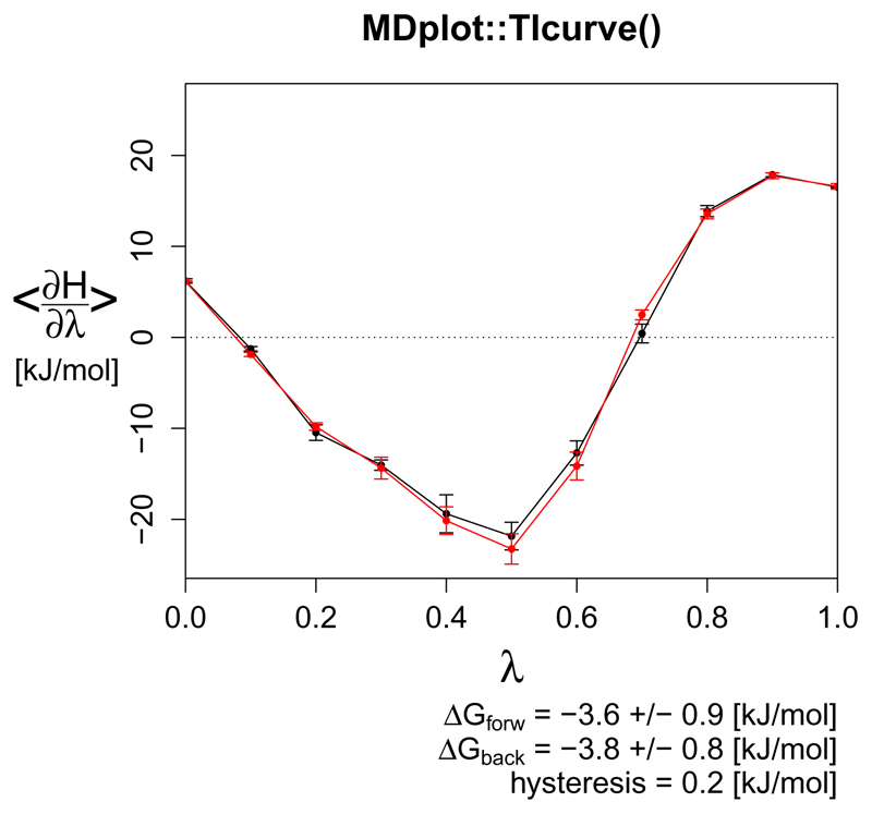
For calculations of the free energy difference occurring when transforming one chemical compound into another (alchemical changes) or for estimates of free energy changes upon binding, thermodynamic integration (Kirkwood, 1935) is one of the most trusted and applied approaches. The derivative of the Hamiltonian, as a function of a coupling parameter λ, is calculated over a series of λ state points (typically around 15). The integral of this curve is equivalent to the change in free energy (Figure 14). The function TIcurve() performs the integration and, if the data for both the forward and backward processes are provided, the hysteresis between them.
Figure 14.
A forward and backward thermodynamic integration curve with the resulting hysteresis between them (precision as permitted by the error).
TIcurve(load_TIcurve(c("inst/extdata/TIcurve_fb_forward_example.txt.gz",
                       "inst/extdata/TIcurve_fb_backward_example.txt.gz")),
        invertedBackwards=TRUE, main="MDplot::TIcurve()")
Return value: Returns a list with the following components:
lambdapoints A list containing a (at least) n × 3-matrix for every data input series.
integrationresults A matrix containing one row of "deltaG" and "error" columns from the integration for every data input series.
hysteresis if two (i.e. forward and backward) data input series are provided, the resulting hysteresis is reported (and set to be NA otherwise).
Table 13.
Arguments of the TIcurve() function.
| Argument name | Default value | Description |
|---|---|---|
| lambdas | none | List of matrices (automatically generated by load_TIcurve()) holding the thermodynamic integration information. |
| invertedBackwards | FALSE | If a forward and backward TI are provided and the lambda points are enumerated reversely (i.e. 0.3 of one TI is equivalent to 0.7 of the other), this flag can be set to be TRUE in order to automatically mirror the values appropriately. |
| energyUnit | "kJ/mol" | Defines the energy unit used for the plot. |
| printValues | TRUE | If TRUE, the free energy values are printed. |
| printErrors | TRUE | A Boolean indicating whether error bars are to be plotted. |
| errorBarThreshold | 0 | If the error at a given lambda point is below this threshold, it is not plotted. |
| barePlot | FALSE | A Boolean indicating whether the plot is to be made without any additional information. |
| … | none | Additional arguments. |
The timeseries() function
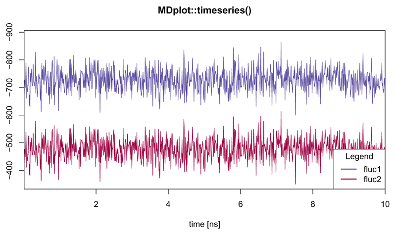
This function provides a general interface for any time series given as a time-value pair (Figure 15).
Figure 15.
Shows time series with parameter snapshotsPerTimeInt set in a way such, that the proper time in nanoseconds is plotted. In addition, the legend has been moved to the bottom-right position.
timeseries(load_timeseries(c("inst/extdata/timeseries_example_1.txt.gz",
                             "inst/extdata/timeseries_example_2.txt.gz")),
           main="MDplot::timeseries()",
           names=c("fluc1","fluc2"),
           snapshotsPerTimeInt=100)
Return value: Returns a list of lists, each of the latter holding for every data input series:
minValue The minimum value over the whole set.
maxValue The maximum value over the whole set.
meanValue The mean value over the whole set.
sd The standard deviation over the whole set.
Table 14.
Arguments of the timeseries() function.
| Argument name | Default value | Description |
|---|---|---|
| tsData | none | List of (alternating) indices and response values, as produced by load_timeseries(). |
| printLegend | TRUE | Parameter enabling the plotting of the legend. |
| snapshotsPerTimeInt | 1000 | Number specifying how many snapshots make up one timeUnit. |
| timeUnit | ”ns” | Specifies the time unit. |
| valueName | NA | Name of response variable. |
| valueUnit | NA | Specifies the response variable's unit. |
| colours | NA | A vector of colours used for plotting. |
| names | NA | A vector of names of the trajectories. |
| legendPosition | ”bottomright” | Indicates position of legend: either ”bottomright”, ”bottomleft”, ”topleft”, or ”topright”. |
| barePlot | FALSE | A Boolean indicating whether the plot is to be made without any additional information. |
| … | none | Additional arguments. |
The xrmsd() function
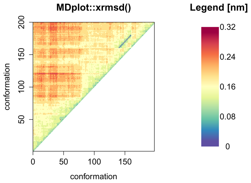
This function generates a plot which shows a heat-map of the atom positional root-mean-square differences between snapshots (figure 16). The structures are listed on the x- and y-axes. The heat-map shows the difference between one structure and another using a coloured bin. The legend is adapted in accordance to the size of the values.
Figure 16.
An example xrmsd() plot showing only the upper half because of the mirroring of the values.
xrmsd(load_xrmsd("inst/extdata/xrmsd_example.txt.gz"),
      printLegend=TRUE,main="MDplot::xrmsd()")
Table 15.
Arguments of the xrmsd() function.
| Argument name | Default value | Description |
|---|---|---|
| xrmsdValues | none | Input matrix (three rows: x-values, y-values, RMSD-values). Can be generated by function load_xrmsd(). |
| printLegend | TRUE | If TRUE, a legend is printed on the right hand side. |
| xaxisRange | NA | A vector of boundaries for the x-snapshots. |
| yaxisRange | NA | A vector of boundaries for the y-snapshots. |
| colours | NA | User-specified vector of colours to be used for plotting. |
| rmsdUnit | ”nm” | Specifies in which unit the RMSD values are given. |
| barPlot | FALSE | A Boolean indicating whether the plot is to be made without any additional information. |
| … | none | Additional arguments. |
Additional functions and the Bash interface
Given that the plotting functions expect input to be stored in a defined data structure, the step of loading and parsing data from the text input files has been implemented in separate loading functions. Currently, they support GROMOS, GROMACS, and AMBER file formats and further developments are planned to cover additional ones as well.
In order to allow for direct calls from Bash scripts, users might use the Rscript interface located in the folder ′bash′ which serves as a wrapper shell. Pictures in the file formats PNG, TIFF, or PDF can be used provided that the users′ R installation supports them. If help=TRUE is set, all the other options are ignored and a full list of options for every command is printed. In general, the names of the arguments of the functions are the same for calls by script. The syntax for these calls is Rscript MDplot_bash.R {function name} [argument1=...] [argument2=...], which can be combined with Bash variables (see below). The file path can be given in an absolute manner or relative to the Rscript folder path. The package holds a file called ′bash/test.sh′ which contains several examples.
#/bin/bash
# clusters
Rscript MDplot_bash.R clusters files=../extdata/clusters_example.txt.gz \
                               title="Cluster analysis" size=900,900 \
                               outformat=tiff outfile=clusters.tiff \
                               clustersNumber=7 \
                               names=WT,varA,varB,varC2,varD3,varE4

# xrmsd
Rscript MDplot_bash.R xrmsd files=../extdata/xrmsd_example.txt.gz title="XRMSD" \
                            size=1100,900 outformat=pdf outfile=XRMSD.pdf \
                            xaxisRange=75,145

# ramachandran
Rscript MDplot_bash.R ramachandran files=../extdata/ramachandran_example.txt.gz \
                      title="Ramachandran plot" size=1400,1400 resolution=175 \
                      outformat=tiff outfile=ramachandran.tiff angleColumns=1,2 \
                      bins=75,75 heatFun=norm printLegend=TRUE plotType=fancy
The loading functions
In order to ease data preparation, loading functions have been devised which are currently able to load the output of standard GROMOS, GROMACS, and AMBER analysis tools and store these data such, that they can be interpreted by the MDplot plotting functions.2 Loading functions are named after their associated plotting function with 'load_' as prefix. For other molecular dynamics engines than the aforementioned ones, the user has to specify how their output should be read. However, in case other file formats are requested we appreciate suggestions, requests, and contributions (to be made on our GitHub page). For detailed descriptions of the data structures used, we refer to the manual pages of the loading functions and the respective examples. For storage reasons the example input files have been compressed using gzip with R being able to load both compressed and uncompressed files.
Conclusions
In this paper we have presented the package MDplot and described its application in the context of molecular dynamics simulation analysis. Automated figure generation is likely to aid in the understanding of results at the first glance and may be used in presentations and publications. Planned extensions include both the integration of new functionalities such as a DISICL (secondary structure classification (Nagy and Oostenbrink, 2014a,b)) as well as the provision of loading interfaces for additional molecular dynamics engines. Further developments will be published on the projects′ GitHub page and on CRAN.
Figure 12.
In black, the mean RMSD value at a given timepoint and in grey the respective minimum and maximum values are given. In this example, two rather similar curves have been used.
Acknowledgements
The authors would like to thank Prof. Friedrich Leisch for his useful comments and guidance in the package development process, Markus Fleck for providing GROMACS analysis files, Silvia Bonomo for her help in dealing with AMBER, Sophie Krecht for her assistance in typesetting, and Jamie McDonald for critical reading of the manuscript.
Funding
This work was supported by the European Research Council (ERC; grant number 260408), the Austrian Science Fund (FWF; grant number P 25056) and the Vienna Science and Technology Fund (WWTF; grant number LS08-QM03).
Footnotes
In this manuscript, the code samples use GROMOS input (since the default value of the loading functions′ parameter mdEngine is ”GROMOS”). For information on how to load GROMACS or AMBER files, please have a look at the manual pages of the respective loading functions.
Functions load_timeseries() and load_TIcurve() do not require engine-specific loading and function noe() is only available for GROMOS because no input files for the other engines could be retrieved.
Bibliography
- Berman HM, Westbrook J, Feng Z, Gilliland G, Bhat TN, Weissig H, Shindyalov IN, Bourne PE. The Protein Data Bank. Nucleic Acids Research. 2000;28(1):235. doi: 10.1093/nar/28.1.235. [DOI] [PMC free article] [PubMed] [Google Scholar]
- Brooks BR, Brooks CL, MacKerell AD, Nilsson L, Petrella RJ, Roux B, Won Y, Archontis G, Bartels C, Boresch S, Caflisch A, et al. CHARMM: The Biomolecular Simulation Program. Journal of Computational Chemistry. 2009;30(10):1545–1614. doi: 10.1002/jcc.21287. ISSN 0192-8651. [DOI] [PMC free article] [PubMed] [Google Scholar]
- Comoglio F, Rinaldi M. Rknots: Topological analysis of knotted biopolymers with R. Bioinformatics. 2012;28(10):1400. doi: 10.1093/bioinformatics/bts160. [DOI] [PubMed] [Google Scholar]
- Cornell WD, Cieplak P, Bayly CI, Gould IR, Merz KM, Ferguson DM, Spellmeyer DC, Fox T, Caldwell JW, Kollman PA. A Second Generation Force Field for the Simulation of Proteins, Nucleic Acids, and Organic Molecules. Journal of the American Chemical Society. 1995;117(19):5179–5197. doi: 10.1021/ja00124a002. ISSN 0002-7863. [DOI] [Google Scholar]
- Eichenberger AP, Allison JR, Dolenc J, Geerke DP, Horta BAC, Meier K, Oostenbrink C, Schmid N, Steiner D, Wang D, van Gunsteren WF. GROMOS++ Software for the Analysis of Biomolecular Simulation Trajectories. Journal of Chemical Theory and Computation. 2011;7(10):3379–3390. doi: 10.1021/ct2003622. ISSN 1549-9618. [DOI] [PubMed] [Google Scholar]
- Grant BJ, Rodrigues APC, ElSawy KM, McCammon JA, Caves LSD. Bio3d: An R package for the comparative analysis of protein structures. Bioinformatics. 2006;22(21):2695–2696. doi: 10.1093/bioinformatics/btl461. ISSN 1367-4803, 1460-2059. [DOI] [PubMed] [Google Scholar]
- Kabsch W, Sander C. Dictionary of protein secondary structure: Pattern recognition of hydrogen-bonded and geometrical features. Biopolymers. 1983;22(12):2577–2637. doi: 10.1002/bip.360221211. ISSN 1097-0282. [DOI] [PubMed] [Google Scholar]
- Kirkwood JG. Statistical mechanics of fluid mixtures. Journal of Chemical Physics. 1935;300 [Google Scholar]
- Margreitter C, Oostenbrink C. Optimization of Protein Backbone Dihedral Angles by Means of Hamiltonian Reweighting. Journal of Chemical Information and Modeling. 2016;56(9):1823–1834. doi: 10.1021/acs.jcim.6b00399. [DOI] [PMC free article] [PubMed] [Google Scholar]
- McGibbon RT, Beauchamp KA, Harrigan MP, Klein C, Swails JM, Hernández CX, Schwantes CR, Wang L-P, Lane TJ, Pande VS. MDTraj: A Modern Open Library for the Analysis of Molecular Dynamics Trajectories. Biophysical Journal. 2015;109(8):1528–1532. doi: 10.1016/j.bpj.2015.08.015. [DOI] [PMC free article] [PubMed] [Google Scholar]
- Nagy G, Oostenbrink C. Dihedral-Based Segment Identification and Classification of Biopolymers II: Polynucleotides. Journal of Chemical Information and Modeling. 2014a;54(1):278–288. doi: 10.1021/ci400542n. [DOI] [PMC free article] [PubMed] [Google Scholar]
- Nagy G, Oostenbrink C. Dihedral-based segment identification and classification of biopolymers I: Proteins. Journal of Chemical Information and Modeling. 2014b;54(1):266–277. doi: 10.1021/ci400541d. ISSN 1549-960X. [DOI] [PMC free article] [PubMed] [Google Scholar]
- Phillips JC, Braun R, Wang W, Gumbart J, Tajkhorshid E, Villa E, Chipot C, Skeel RD, Kalé L, Schulten K. Scalable molecular dynamics with NAMD. Journal of Computational Chemistry. 2005;26(16):1781–1802. doi: 10.1002/jcc.20289. ISSN 1096-987X. [DOI] [PMC free article] [PubMed] [Google Scholar]
- Pronk S, Páll S, Schulz R, Larsson P, Bjelkmar P, Apostolov R, Shirts MR, Smith JC, Kasson PM, van der Spoel D, Hess B, et al. GROMACS 4.5: a high-throughput and highly parallel open source molecular simulation toolkit. Bioinformatics. 2013;29(7):845–854. doi: 10.1093/bioinformatics/btt055. ISSN 1367-4803, 1460-2059. [DOI] [PMC free article] [PubMed] [Google Scholar]
- Ramachandran GN, Ramakrishnan C, Sasisekharan V. Stereochemistry of polypeptide chain configurations. Journal of Molecular Biology. 1963;7:95–99. doi: 10.1016/s0022-2836(63)80023-6. ISSN 0022-2836. [DOI] [PubMed] [Google Scholar]
- Schmid N, Christ CD, Christen M, Eichenberger AP, van Gunsteren WF. Architecture, implementation and parallelisation of the GROMOS software for biomolecular simulation. Computer Physics Communications. 2012;183(4):890–903. doi: 10.1016/j.cpc.2011.12.014. ISSN 0010-4655. [DOI] [Google Scholar]
- Skjærven L, Yao X-Q, Scarabelli G, Grant BJ. Integrating protein structural dynamics and evolutionary analysis with Bio3D. BMC Bioinformatics. 2014;15(1) doi: 10.1186/s12859-014-0399-6. [DOI] [PMC free article] [PubMed] [Google Scholar]


