Cure Modeling in Real-Time Prediction: How Much Does It Help?

Abstract

Various parametric and nonparametric modeling approaches exist for real-time prediction in time-to-event clinical trials. Recently, Chen (2016 BMC Biomedical Research Methodology 16) proposed a prediction method based on parametric cure-mixture modeling, intending to cover those situations where it appears that a non-negligible fraction of subjects is cured. In this article we apply a Weibull cure-mixture model to create predictions, demonstrating the approach in RTOG 0129, a randomized trial in head-and-neck cancer. We compare the ultimate realized data in RTOG 0129 to interim predictions from a Weibull cure-mixture model, a standard Weibull model without a cure component, and a nonparametric model based on the Bayesian bootstrap. The standard Weibull model predicted that events would occur earlier than the Weibull cure-mixture model, but the difference was unremarkable until late in the trial when evidence for a cure became clear. Nonparametric predictions often gave undefined predictions or infinite prediction intervals, particularly at early stages of the trial. Simulations suggest that cure modeling can yield better-calibrated prediction intervals when there is a cured component, or the appearance of a cured component, but at a substantial cost in the average width of the intervals.

1. Introduction

Many clinical trials with time-to-event outcomes schedule interim and final analyses to take place on the occurrence of a pre-specified number of events. For example, a cancer trial could be designed to have 80% statistical power with 300 deaths, with planned interim analyses after the 100th and 200th deaths, and a final analysis when the 300th death occurs [1]. Because the times of occurrence of these landmark events are random, it is desirable to have a tool for predicting them as an aid to logistical planning.

We have developed a range of models for making such predictions [2, 3, 4, 5, 6] and demonstrated their utility in a motivating clinical trial [7]. These models assume that every participant is susceptible and will eventually experience the event if follow-up time is sufficiently long [8, 9]. This assumption may not hold in diseases where there is a possibility of cure — for example, in many childhood cancers and some adult cancers such as leukemia [10, 11], colon cancer [12], and head-and-neck cancer [13]. Failure to accommodate the possibility of cure could in principle lead to bias, because a fraction of surviving patients would be predicted to experience events to which they are effectively no longer susceptible.

Recognizing this gap in the literature, Chen [14] recently proposed the use of cure models [15] in prediction. His method involves, at each prediction time, selecting the best-fitting from among a menu of cure-mixture models (exponential, Weibull, log-logistic and lognormal), and using it to create predicted values for all as-yet unenrolled subjects and all enrolled but censored subjects. He demonstrated the application of his method in a two-arm cancer immunotherapy trial. At every prediction time, goodness-of-fit statistics selected the Weibull cure-mixture model. Initial predictions of the time of the planned final analysis (to be conducted at the 416th death) were as much as 20 months early, but subsequent predictions were closer to the target. Only at the final two (of six) predictions did the empirical survival curve reveal the characteristic shape of the cure model.

Chen presented no evaluation of how his method would perform in repeated samples, either as an estimation or a prediction procedure. Although parametric cure-mixture models are generally identifiable and can be estimated by maximum likelihood with standard asymptotics, they are known to be unreliable in the small-to-moderate sample sizes typically observed in clinical trials [16]. Moreover estimation is particularly challenging when follow-up is short and empirical survival curves have not had time to reach a plateau. Because predictions are of most value early in the trial, which is precisely when no subjects have extended follow-up, there is concern that the mixture-modeling approach may not be helpful in typical practice.

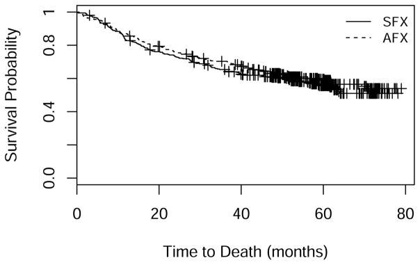
Another motivating example is Radiation Therapy Oncology Group trial 0129 (RTOG 0129) [1], which compared accelerated-fractionation radiotherapy plus concurrent cisplatin-based chemotherapy to standard-fractionation radiotherapy alone among patients with oropharyngeal squamous-cell carcinoma. The study found no statistically significant treatment effect on survival. An interesting feature of the data is that the Kaplan-Meier (KM) curves for both arms level off (Figure 1), suggesting that a large fraction of subjects are effectively cured of their cancer.

Figure 1.

Kaplan-Meier curves in RTOG 0129: SFX = standard-fractionation radiotherapy alone; AFX = accelerated-fractionation radiotherapy plus concurrent cisplatin-based chemotherapy.

In this paper we further explore the Weibull cure-mixture prediction model that provided the best fit in Chen’s immunotherapy trial example. We apply this model, together with a non-cure Weibull model and a nonparametric model, to create and empirically evaluate interim predictions in RTOG 0129. We study the relative performance of the methods in a simulation experiment.

2. Methods

2.1. General framework for event-time prediction

We briefly review the prediction framework described in detail in [2, 3, 4, 7, 8]. Assume we are conducting a two-arm randomized trial that began enrolling patients at calendar time 0. Subjects arrive according to a Poisson process with a constant rate of μ per unit of time and are randomized 1:1 between study arms. Each participant can either i) develop the event of interest, ii) remain in the trial without occurrence of the event, or iii) become lost to follow-up. At current calendar time t₀ > 0 we seek to make predictions about the future course of the trial. A typical objective is to predict the calendar time T^* at which the D^*th event will occur; for example, at t₀ = 6 months we may predict the time T^* at which event D^* = 100 will occur. The essence of the method is to use the accumulating trial data to estimate the accrual/survival model, which we then use to create predictions about the future course of the trial.

We previously developed a Bayesian prediction method based on a Weibull (non-cure) survival model [4], which assumes that survival time T in arm j, j = 0, 1 follows the survival function

$$Pr[T>t]=S(t\mid {\alpha }_j,{\beta }_j)=exp[-{(t/{\beta }_j)}^{{\alpha }_j}],t>0,{\alpha }_j>0,{\beta }_j>0,$$ (1)

and that time to loss to follow-up in arm j independently follows a Weibull with arm-specific scale and shape parameters. The first step in the prediction modeling is to specify priors for the enrollment rate and the parameters of the Weibull event and loss to follow-up distributions in each arm. To create predictions at time t₀ we compute the posterior density of the parameters using the data accrued up to that time. Then we conduct the following steps many times:

1. Sample a set of parameters from the posterior using importance sampling (or some other method).

2. Conditional on the sampled parameters, sample a data set from the predictive distribution of the enrollment, survival and loss times:

   1. Simulate the event and loss to follow-up times for participants who are enrolled and on study but have not yet experienced an event.

   2. If the total enrollment goal has not yet been reached, simulate the enrollment, event and loss times for a hypothetical set of participants who have not yet been enrolled.

   3. Determine each subject’s date of event or loss (real or simulated), and rank the event dates among subjects who either have had an event or are predicted to have an event.

   4. Identify the date of the landmark time T^*.

Each replication of steps 1 and 2 generates a draw from the predictive distribution of the landmark time T^*. Repeating them many times, one can predict the landmark time as, for example, the median of the simulated distribution of T^*, with 95% prediction interval equal to the interval between the 2.5th and 97.5th centiles of the simulated distribution.

2.2. Prediction using the Weibull cure-mixture model

Common failure-time models assume that every subject is susceptible to the event of interest and will experience it if followed long enough. This assumption fails in studies where there is a possibility of cure. The cure-mixture model addresses this deficiency by positing that the study sample is a mixture of uncured individuals (who will experience the event of interest if not censored) and cured individuals (who will never experience it no longer how long we follow them) [15, 16, 17, 18]. Let T denote the time to the event of interest. The Weibull cure-mixture model asserts that for a subject in arm j,

$$Pr[T>t]=(1-{\rho }_j)\times S(t\mid {\alpha }_j,{\beta }_j)+{\rho }_j,$$ (2)

where S(t|α_j, β_j) is the Weibull survival function from Equation (1), and ρ_j ∈ [0, 1] is the probability of cure in arm j. When t is large, the survival function approaches the cure fraction ρ_j; when ρ_j = 0, it reduces to the standard Weibull survival model.

Many variations of the cure-mixture model appear in the literature [19]. A common version models the cure probability with a logistic regression and the survival with a Weibull distribution, the latter being a popular choice thanks to its flexibility and its similarity to Cox regression [20]. Our analyses will model both the cure probability and the Weibull survival parameters only as functions of the randomization arm (see Equation 2).

Under the Weibull cure-mixture model the overall prediction framework remains the same, except that one must also predict cure status for the censored and not-yet-enrolled subjects. We generate the cure status of each unenrolled participant in arm j by binomial sampling with the sampled cure probability ρ̃_j. For a subject in arm j who was enrolled at calendar time e, and who did not experience an event by prediction time t₀ ≥ e, the conditional cure probability for sampling is

$$\stackrel{\sim }{Pr}[\text{cured}\mid T>t_0-e]=\frac{{\stackrel{\sim }{\rho }}_j}{{\stackrel{\sim }{\rho }}_j+(1-{\stackrel{\sim }{\rho }}_j)\times S(t_0-e;{\stackrel{\sim }{\alpha }}_j,{\stackrel{\sim }{\beta }}_j)},$$ (3)

where S(·; α̃_j, β̃_j) is the Weibull survival function given sampled parameters α̃_j and β̃_j. The cure status for these already enrolled subjects in arm j is then simulated from the binomial distribution with this estimated cure probability. For a subject who is simulated to be cured, the event time is imputed as infinity. If a subject is simulated as not cured, we impute the event time by drawing from the unconditional Weibull for a new subject, or the Weibull conditional on the event time being at least t₀ – e for an existing censored subject.

Our prediction approach is Bayesian and therefore requires specification of a prior for the model parameters. We describe the selection of priors for RTOG 0129 in §4.3 below.

2.3. The nonparametric prediction model

Ying et al. [3] have described a nonparametric (NP) approach to prediction that proceeds according to the following steps:

1. Re-sample the data by the Bayesian bootstrap (BB) [21].

2. Create a draw from the posterior of the survival curve under a nonparametric model by computing the KM curve from the resampled data.

3. Conditional on the resampled KM curve, sample a data set from the predictive distribution of the data:

   1. Simulate the event and loss to follow-up times for participants who are enrolled and on study but have not yet experienced an event.

   2. If the total enrollment goal has not yet been reached, simulate the enrollment, event and loss times for a hypothetical set of participants who have not yet been enrolled.

   3. Determine each subject’s date of event or loss (real or simulated), and rank the event dates among subjects who either have had an event or are predicted to have an event.

   4. Identify the date of the landmark time T^*.

2.4. Infinite event times

In the cure-mixture model, we represent a cured individual mathematically as having an infinite event time. When the event is death, of course a cure is impossible — nobody lives forever. Rather, we interpret the infinite event time as meaning that the subject dies at a more advanced age, potentially from another disease than the one under study. In that sense the cure-mixture model is only ever an approximation.

The possibility of infinite event times has important ramifications for prediction algorithms, because in a given set of imputed event times it is possible that the predicted time of the event landmark T^* will itself be infinite. This would occur if we were attempting to predict the time of the D^*th event, but the set of imputed event times had fewer than D^* finite event times. Thus in a given simulated predictive distribution it is possible for the upper limit of the prediction interval, the median prediction, and even the lower limit of the prediction interval to be infinite.

In model-based predictions, one generates an infinite event time by a successful draw with probability $\stackrel{\sim }{Pr}[\text{cured}\mid T>t_0-e]$ in Equation 3. In the NP prediction model, there is no assumed cure probability, but the simulation procedure can generate an infinite event time when the largest event time in the BB sample is censored, because in this case the curve effectively has a mass at infinity. In the original version of our NP prediction model [3], we sought to avoid generating infinite event times, and thus we followed the common practice of appending a parametric tail to the KM curve whenever the largest re-sampled event time was censored. When, as in RTOG 0129, cure is a possibility, one may wish to preserve the possibility of generating infinite event times. We accomplished this easily by simply not appending a tail when the BB KM curve does not decline to zero. Thus this simplified version of the NP method naturally accounts for cures.

3. Simulations

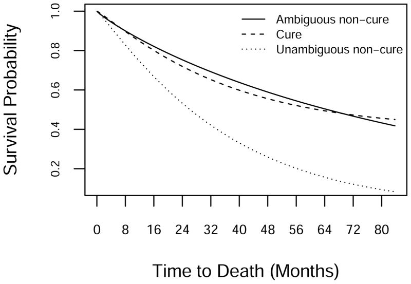
We conducted a simulation study to evaluate performance of the methods under a range of scenarios inspired by the RTOG 0129 experience. Table 1 presents the parameters of the survival model used in the simulations, and Figure 2 displays the implied survival curves. The first set of parameters, referred to as the “Cure” model, is similar to the estimates from RTOG 0129 under the Weibull cure-mixture model. The second set, “Ambiguous Non-Cure”, roughly equals the estimates from the data assuming a Weibull model with zero cure fraction. This distribution has long tails and is indistinguishable from a cure model under the RTOG 0129 follow-up regime. The third set, “Unambiguous Non-Cure”, equals estimates from the Weibull portion of the cure model, but with cure fraction set to 0. A survival curve generated under this scenario declines to near 0 under RTOG 0129 follow-up, and therefore will inform us on how the methods perform when a cure model is unnecessary.

Table 1.

Parameters for generating data in the simulations.

Parameter	Scenario
	Cure	Ambiguous Non-Cure	Unambiguous Non-Cure
ρ	0.4	0	0
α	1.1	0.9	1.1
β	3.0	8.0	3.0

Figure 2.

Survival curves for generating the simulation data.

Our simulated two-arm trial enrolled an expected 721 patients, arriving over 1,080 days according to a Poisson process, assuming a total length of follow-up of 2,512 days. We assumed that survival times were the same in both arms, and that times of loss to follow-up were Weibull with parameters that would lead to only rare losses in a trial like RTOG 0129.

We created predictions under the three models indicated above. For each of 100 simulated data sets, we predicted the dates of the 300th event by each method using data as of the occurrence of the 75th, 150th and 225th events (looks 1, 2, and 3, respectively). The expected dates for creating these predictions are approximately 740, 1,110 and 1,500 days for ambiguously non-cure data; 710, 1,030, and 1,550 days for cure-mixture data; and 550, 800 and 982 days for unambiguously non-cure data. For each method, we calculated the median width of the 95% prediction interval and its coverage probability. We also calculated an estimate of the cure probability — its posterior mode — under the Weibull cure-mixture method.

Table 2 shows results of the simulation under the true cure model. As expected, the cure-mixture method performs reasonably well, with coverage rates around 90%. The non-cure method gives much shorter but badly calibrated intervals, with coverage ranging from 27% to 43%. The NP method produces large numbers of imputed times at infinity; in fact, under this scenario none of the simulated intervals was of finite width. Its coverage probabilities improve from 25% at the first look to 92% at the third.

Table 2.

Prediction performance under the cure-mixture scenario.

Look	Median interval width (days)			Coverage rate (%)
	Cure	Non-cure	NP	Cure	Non-cure	NP
1	680	306	∞*	92	27	25
2	422	227	∞*	87	31	55
3	279	171	∞*	90	43	92

^*All 100 intervals had infinite width.

Table 3 shows results under the scenario of ambiguously non-cure data. The cure model again performs best, even though the simulated data contain no actual cures. The Weibull non-cure model gives shorter intervals that are poorly calibrated initially but improve at later looks. Again, the NP method sees the data essentially as cure data and produces infinite intervals for all 100 simulations, giving reliable intervals only at the third look.

Table 3.

Prediction performance under the ambiguous non-cure scenario.

Look	Median interval width (days)			Coverage rate (%)
	Cure	Non-cure	NP	Cure	Non-cure	NP
1	1298	336	∞*	98	36	14
2	702	272	∞*	94	56	53
3	363	211	∞*	97	82	83

^*All 100 intervals had infinite width.

Table 4 shows results under the unambiguously non-cure scenario. Here the Weibull non-cure method gives the shortest intervals and is reasonably well calibrated. The cure-mixture method works almost as well, giving intervals that are nearly as well calibrated but somewhat longer. The NP method is ineffective at the first look but improves thereafter.

Table 4.

Prediction performance under the unambiguous non-cure scenario.

Look	Median interval width (days)			Coverage rate(%)
	Cure	Non-cure	NP	Cure	Non-cure	NP
1	358	238	∞*	79	88	53
2	178	148	∞†	90	97	88
3	102	92	150	92	94	97

^*All 100 intervals had infinite width.

^†Seventy-seven of 100 intervals had infinite width.

The median estimated cure probabilities and their 2.5th and 97.5th centiles appear in Table 5. Recall that under the cure model for generating the data, the cure fraction was 0.4; under the non-cure models it was zero. When the data contain cures, the probabilities are underestimated somewhat but not too far off, with median values ranging from 11% at the early look to 25% at the last look. With ambiguous non-cure data, the cure model was easily fooled, with average estimated cure probabilities of 20% or more. With unambiguously non-cure data the cure model estimated cure probabilities at on average 10% or less.

Table 5.

Summary of the distribution of the estimated (posterior mode) cure probability.

Look/Model	2.5th centile	Median	97.5th centile
Cure-mixture (ρ = 0.4)
1	0.05	0.11	0.13
2	0.06	0.16	0.18
3	0.06	0.25	0.46
Ambiguous non-cure (ρ = 0)
1	0.08	0.20	0.42
2	0.10	0.26	0.42
3	0.07	0.26	0.42
Unambiguous non-cure (ρ = 0)
1	0.04	0.06	0.11
2	0.03	0.06	0.34
3	0.02	0.05	0.32

4. Prediction in RTOG 0129

4.1. RTOG 0129

RTOG 0129 was a phase III trial to evaluate whether accelerated-fractionation radiotherapy with concurrent cisplatin-based chemotherapy (AFX) improves survival compared to standard-fractionation radiotherapy alone (SFX) in stage III or IV squamous-cell carcinoma of the head and neck [1]. The primary outcome was time to death from any cause. A sample size calculation informed by data from prior studies indicated that 309 deaths would give 80% power (in a one-sided test with type I error rate 5%) to detect a 25% reduction in the hazard of death (giving 2-year mortality of 45% on AFX vs. 55% on SFX). Investigators planned to conduct interim analyses at deaths 103 and 206, with a final analysis after death 309. With accrual projected at 13 patients/month, the trial was expected to achieve 309 deaths by enrolling 456 analyzable patients in three years and following them for an additional two years.

Enrollment began on September 18, 2002. By May 2004 the trial had accrued roughly 400 patients, or nearly double its expected number by that date. Therefore RTOG amended the protocol to increase the total sample size to 684 patients, which would give 80% power for a reduction of 20% in the death hazard. The revised sample size was projected to be accrued within three years of the trial’s opening. The analysis plan was accordingly modified to require 584 deaths, with interim analyses after deaths 184 and 369. At the close of enrollment on June 23, 2005, the trial had enrolled 721 eligible patients. Enrollment took 1009 days (2.8 years), at an average rate of 22 subjects/month.

In January 2007 the trial’s Data & Safety Monitoring Board (DSMB) reviewed the first interim analysis, derived from a data set containing the initial 192 deaths. The estimated overall two-year mortality rate was 28%, far lower than the assumed rates of 55% for SFX and 45% for AFX from the sample size calculation. Assuming exponential survival, RTOG statisticians projected that the second interim analysis would not take place until June 2013.

In light of the unexpectedly low death rate, in June 2008 RTOG again re-evaluated the analysis plan. With 257 deaths to date, the second interim analysis was projected to take place in January 2011 — earlier than had been predicted in January 2007 but far beyond the original planned closing date. Because RTOG 0129 was one of the first large trials to test the potentially highly toxic AFX regimen, radiation oncologists anxiously awaited its results. In order to spare patients unnecessary toxicity during a lengthy follow-up, RTOG reverted to the original plan of closing the study after death 309. Because the number of deaths recorded at this juncture (257) exceeded the original number designated for the second analysis (206), the second interim analysis was omitted.

The trial was closed in May 2009 with the occurrence of the 303rd death. The 103rd death took place on April 16, 2005 (day 940), the 206th death on October 22, 2006 (day 1,494), and the 303rd death on May 12, 2009 (day 2,427) (Table 6). No participant was lost to follow-up.

Table 6.

Evolution of RTOG 0129.

t0		Trial Progress		Treatment Effect
Date	Months	Enrollment	Deaths	ln(HR)	Logrank P
01/17/2003	4	39	1	NA	NA
05/17/2003	8	119	6	1.69	0.08
09/14/2003	12	211	10	0.43	0.50
01/12/2004	16	302	22	0.02	0.96
05/11/2004	20	398	34	−0.01	0.99
09/08/2004	24	483	56	0.22	0.41
01/06/2005	28	573	78	−0.15	0.50
04 /16 /2005	31.3	665	103	−0.22	0.27
05/06/2005	32	688	111	−0.14	0.47
09/03/2005	36		136	−0.13	0.46
01/01/2006	40		160	−0.11	0.47
05/01/2006	44		182	−0.17	0.25
08/29/2006	48		196	−0.18	0.20
10 /22 /2006	49.8		206	−0.16	0.26
12/27/2006	52		217	−0.14	0.30
04/26/2007	56		233	−0.10	0.44
08/24/2007	60		247	−0.11	0.37
12/22/2007	64		261	−0.14	0.26
04/20/2008	68		272	−0.13	0.29
08/18/2008	72		284	−0.11	0.35
12/16/2008	76		290	−0.14	0.24
04/15/2009	80		297	−0.10	0.40
05 /12 /2009	80.9		303	−0.10	0.37

HR=hazard ratio. Italicized rows represent planned analysis times.

4.2. Prediction of time to reach landmark events

We applied three models — NP, Weibull, and Weibull cure-mixture — to predict the times to reach deaths 103, 206, and 303. We created predictions retrospectively at two-month intervals, starting 8 months from the opening of the study, using only data available at the time of prediction. (Month 8 was the first point at which each arm had at least one death.) We first made predictions for the time of death 103; at time points after its occurrence we made predictions for death 206; and after its occurrence we made predictions for death 303. In addition to the time to reach the landmark event count, we computed the predicted treatment effect and the predictive power, or Bayesian probability that the trial results would be statistically significant [7, 23, 24]. To compute the latter, we constructed each simulated data set as it would have existed at each future analysis time, and calculated the fraction of such simulated data sets for which the trial’s sequential testing procedure would yield statistical significance. The critical values for statistical significance from the one-sided logrank test using the O’Brien-Fleming α-spending function approach were Z = (3.20, 2.14, 1.69) at the three looks, respectively, or alternatively one-sided P = (0.00069, 0.01569, 0.03363).

Rcode is available upon request from the last author.

4.3. Priors for the prediction models

For parameter specification, we measured all times in units of years. For accrual rate, we assumed the prior Gamma(13, 30/365.25), which is equivalent to one month of data in which 13 patients are accrued, as implied by the original study design. For Weibull shape parameters for event and loss distributions in both arms, we assumed Gamma(1.5,1) priors (i.e., exponential priors with mean 1.5). For the time-to-death distributions, we chose priors for the Weibull scale parameters to give mean values that would roughly match values from pilot data: Gamma(5.6,1) for the scale in the SFX arm and Gamma(7.3,1) for the scale in the AFX arm. Although there was no loss to follow-up either in pilot data or RTOG 0129, to allow for the possibility of losses we assumed priors that gave prior means of 10 years for time to loss to follow-up — specifically, Gamma(11.1,1) in both arms. We took the logits of the cure probabilities to be Cauchy with median 0 and scale 2.5 in both arms. We assumed all parameters to be a priori independent.

4.4. Results

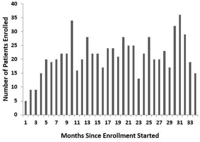
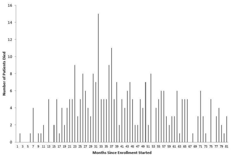
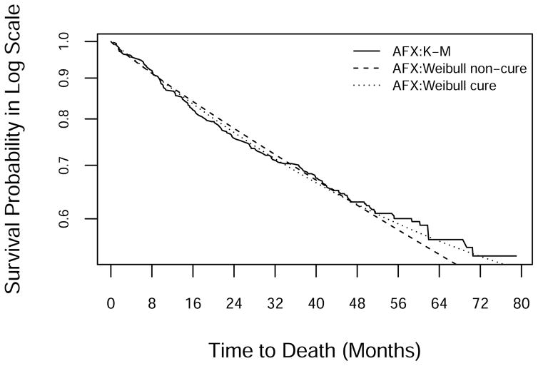
After a brief ramp-up, enrollment settled at around 22 patients per month (Figure 3). Monthly mortality was low initially, reached its highest levels around the time of the close of accrual, and then gradually declined (Figure 4). KM survival curves (Figure 1) suggest that a fraction of subjects are cured, with a tail that flattens out at roughly 50% survival in each arm. Analysis using the Weibull cure model estimated the cure rates to be 49% (95% CI: 40%–58%) on SFX and 46% (95% CI: 31%–61%) on AFX. Goodness-of-fit statistics (Table 7) and graphs (Figure 5) based on the full data set indicate that the Weibull cure model fit marginally better than the standard Weibull.

Figure 3.

Number of subjects enrolled in each month (30-day interval) during the accrual period.

Figure 4.

Number of deaths in each month (30-day interval) during the trial.

Table 7.

Comparison of goodness of fit for the Weibull and Weibull cure-mixture models.

	Goodness-of-fit statistics
Survival model	AIC	AICC	BIC
Standard Weibull	1894.4	1894.4	1908.2
Weibull cure-mixture	1884.1	1884.2	1907.0

AIC = Akaike information criterion; AICC = Corrected Akaike information criterion; BIC = Bayesian information criterion; smaller values represent better fit.

Figure 5.

Log-scale KM and fitted survival curves from the standard and cure-mixture Weibull models in the AFX arm. Curves for the SFX arm were similar.

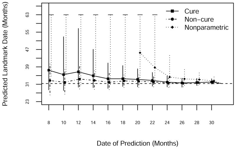
Predictions of death 103, which occurred on day 940, appear in Figure 6. All three models predicted that the event would take place later than it actually did, right up until the time of its occurrence. The standard Weibull model did slightly better than the Weibull cure-mixture. The NP method predicted infinity for much of the early going; the point prediction (the median of the simulated distribution of times to the target event) was infinite until month 20, and the upper limit of the interval (the 97.5th centile of the distribution of times to the target event) was infinite until month 24. The 95% prediction limits from all three approaches cover the actual date; intervals are generally shortest for the Weibull model, somewhat longer for the Weibull cure model, and longest (even when finite) for the NP model. The erroneous predictions by all three methods presumably reflect the increasing rates of monthly mortality observed during the period leading up to event 103; the predictions overshoot the target because the methods consistently underestimate mortality.

Figure 6.

Prediction of the 103rd death using NP, standard Weibull and Weibull cure-mixture models. The horizontal dashed line is the date of occurrence of the 103rd death.

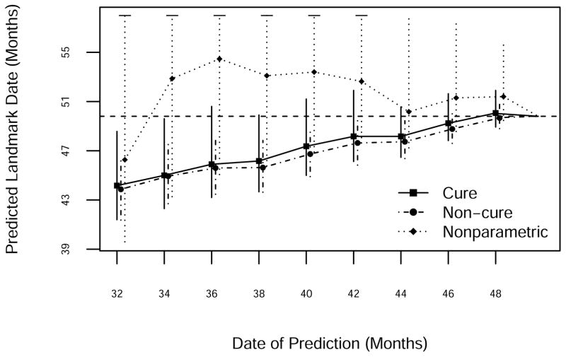
Death 206 took place on study day 1,494 (Figure 7). Both Weibull models predicted that it would occur earlier than it did, presumably reflecting a delayed response to the declining study death count after month 32. Of the three methods the NP was generally the most accurate, although its prediction intervals were infinite prior to month 44. The two parametric methods gave similar predictions, with perhaps a slight advantage for the cure model.

Figure 7.

Prediction of the 206th death using NP, standard Weibull and Weibull cure-mixture models. The horizontal dashed line is the date of occurrence of the 206th death.

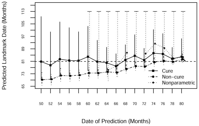
Death 303 occurred on study day 2,427 (Figure 8). By the time of the planned second interim analysis (which never took place thanks to the shifting study design), presumably there was some evidence of a cure fraction. Thus the standard Weibull model, which did not account for cure, gave substantially early predictions until just before event 303. The Weibull cure model did much better initially, although later predictions overshot the target somewhat. NP prediction intervals for this event were again infinite, reflecting the large fraction of evidently cured patients. Thus if one were more concerned with predictions six months or more prior to the ultimate event, the cure model gave correct but fuzzy predictions, whereas within six months of the event the non-cure predictions were correct and had much smaller intervals. NP predictions never dominated either parametric alternative.

Figure 8.

Prediction of the 303rd death using NP, standard Weibull and Weibull cure-mixture models. The horizontal dashed line is the date of occurrence of the 303rd death.

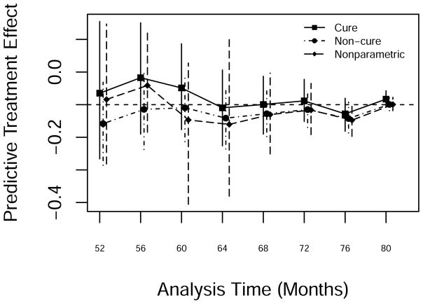
A plot of predictive treatment effect estimates after month 52 from the three approaches appears in Figure 9. All three predictions showed a modest treatment effect. The cure-mixture model gave the best predictions after about month 60.

Figure 9.

Predicted treatment effect from NP, standard Weibull and Weibull cure-mixture models after the occurrence of the 206th death.

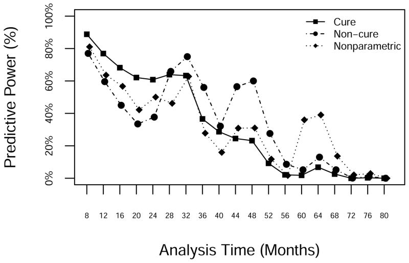
Figure 10 displays the evolution of the predictive power. All three models showed similar patterns, with occasional spikes (months 30, 47 and 64) representing moments when the evidence suggested a possible advantage for AFX. The predictive power declined over time until reaching 0 when the final analysis showed no significant difference between arms. The NP model was the most sensitive to small clusters or droughts in events.

Figure 10.

Predictive power from the NP, standard Weibull and Weibull cure-mixture models, by study month.

5. Discussion

In this and previous articles [2, 3, 4, 5, 6, 7, 8, 9], we have demonstrated that real-time prediction in event-based trials can ease logistical planning, inform interim design decisions, and assist DSMBs in evaluating futility. These elements contribute to the optimal allocation of trial resources and efficient trial operation.

We followed Chen [14] in applying a Weibull cure-mixture model to RTOG 0129. Judged retrospectively, the cure model yielded moderately better predictions than a non-cure model, especially after the data came to suggest a substantial cure fraction. Because the need for cure modeling may become apparent only after many subjects have accrued substantial follow-up time, in general the relative advantage of cure modeling is unlikely to be realized until later in the trial.

Chen did not evaluate the performance of cure-based prediction in repeated samples, a gap that we have addressed here through simulation studies. Our results demonstrate that incorporating a cure model can substantially improve the correctness of predictions if the data suggest that such a model is plausible. Only when the true survival curves decline to near zero over the proposed follow-up does a non-cure model give good prediction coverage. The cost of the improved coverage is substantial, as intervals under the cure model are on average roughly twice as wide in the early going. The NP approach that does not constrain survival curves to decline to zero was practically useless in scenarios where the cure fraction was substantial. Our simulations of the estimated cure fractions reflect the well-known difficulty of estimating such parameters in small-to-moderate samples [16]. Fortunately, it is apparently not necessary to estimate the cure fraction accurately to obtain calibrated prediction intervals.

In principle, no true cure is possible with time to death as the outcome, because even subjects who are cured of the proximal life-threatening disease will eventually die of another cause. Thus modeling cures may be most appropriate in trials for potentially fatal diseases of children, where subjects whose treatment is successful stand to survive for many decades. The good fit of the cure assumption was surprising in RTOG 0129, where the median age at enrollment exceeded 50 and the oldest patient was 82 [1]; at the design stage, RTOG did not anticipate a substantial cure fraction. Nevertheless, the survival curves in Figure 1 suggest that in both arms roughly half of the subjects were effectively cured of the life-threatening effects of their tumors. Allowing the cure fraction to depend on baseline predictors such as age, stage, smoking, and HPV status could improve the accuracy of model-based prediction methods.

A second observation from RTOG 0129 is that trends in mortality strongly influence predictions. When mortality is increasing (decreasing), predictions will overshoot (undershoot) the target, as we saw in the predictions of events 103 and 206. This appears to hold independently of the model being applied, except that the NP method is the most sensitive to small changes in mortality experience. Ying and Heitjan [7] observed a similar phenomenon in REMATCH, where death count predictions strongly reflected a decline in mortality that took hold between the second and third interim analyses.

In addition to predicted treatment effects and predictive power, a further possible byproduct of predictive cure modeling is individual estimated cure probabilities, based on simulation replicates of the values in Equation 3. One could sharpen such predictions by including other variables besides treatment arm in the model for the cure probability.

We have observed that the predicted event rate can be sensitive to the observed enrollment pattern, which suggests that the introduction of flexible models for changing enrollment rates could improve predictions. It is difficult to model changes in the enrollment rate, however, because such changes occur in real (calendar) time and can be difficult to anticipate. Nevertheless, some enrollment trends appear to hold generally, such as a gradual increase in the early months, followed by a period of steady accrual, possibly concluding with a rapid uptick as the trial enters its “home stretch” [28, 29]. We intend to address these issues in future papers.

Model fit is always a concern in parametric survival analysis, and especially so in predictive modeling, which requires extrapolation into the future. Monte Carlo results in Ying et al. [4] suggest that predictions based on the Weibull offer a reasonable compromise between accuracy and efficiency, and therefore we have used them as the basis of our cure-mixture approach. Another alternative is the piecewise exponential model, as applied in the prediction context by Fang and Su [30]. A further possibility would be to use piecewise-constant hazard models where change points are situated at the calendar times of significant events that occur in the trial. For example, in the device arm of REMATCH, the survival experience changed dramatically between the second and third interim analyses, possibly reflecting the implementation of an upgraded infection-control protocol [7]. One could also model such effects via time-varying predictors in survival models.

In summary, predictive cure modeling is a potentially valuable adjunct to planning and decision-making in clinical trials. We anticipate an increased need for such tools as our ability to personalize the treatment of chronic diseases, and thereby effect cures, advances.

References

- 1.Ang KK, Harris J, Wheeler R, Weber R, Rosenthal DI, et al. Human papillomavirus and survival of patients with oropharyngeal cancer. New England Journal of Medicine. 2010;363:24–35. doi: 10.1056/NEJMoa0912217. [DOI] [PMC free article] [PubMed] [Google Scholar]
- 2.Bagiella E, Heitjan DF. Predicting analysis times in randomized clinical trials. Statistics in Medicine. 2001;20:2055–2063. doi: 10.1002/sim.843. [DOI] [PubMed] [Google Scholar]
- 3.Ying GS, Heitjan DF, Chen TT. Nonparametric prediction of event times in randomized clinical trials. Clinical Trials. 2004;1:352–361. doi: 10.1191/1740774504cn030oa. [DOI] [PubMed] [Google Scholar]
- 4.Ying GS, Heitjan DF. Weibull prediction of event times in randomized clinical trials. Pharmaceutical Statistics. 2008;7:107–120. doi: 10.1002/pst.271. [DOI] [PubMed] [Google Scholar]
- 5.Donovan JM, Elliott MR, Heitjan DF. Predicting event times in clinical trials when treatment arm is masked. Journal of Biopharmaceutical Statistics. 2006;16:343–356. doi: 10.1080/10543400600609445. [DOI] [PubMed] [Google Scholar]
- 6.Donovan JM, Elliott MR, Heitjan DF. Predicting event times in clinical trials when randomization is masked and blocked. Clinical Trials. 2007;4:481–490. doi: 10.1177/1740774507083390. [DOI] [PubMed] [Google Scholar]
- 7.Ying GS, Heitjan DF. Prediction of event times in the REMATCH Trial. Clinical Trials. 2013;10:197–206. 1–90. doi: 10.1177/1740774512470314. [DOI] [PubMed] [Google Scholar]
- 8.Heitjan DF, Ge Z, Ying GS. Real-time prediction of clinical trials enrollment and event counts: A review. Contemporary Clinical Trials. 2015;45:26–33. doi: 10.1016/j.cct.2015.07.010. [DOI] [PubMed] [Google Scholar]
- 9.Zhang X, Long Q. Modelling and prediction of subject accrual and event times in clinical trials: A systematic review. Clinical Trials. 2012;9:681–688. doi: 10.1177/1740774512447996. [DOI] [PubMed] [Google Scholar]
- 10.Bennett JM, Andersen JW, Cassileth PA. Long-term survival in acute myeloid leukemia: The Eastern Cooperative Oncology Group (ECOG) experience. Leukemia Research. 1991;15:223–227. doi: 10.1016/0145-2126(91)90124-c. [DOI] [PubMed] [Google Scholar]
- 11.Wang ZY, Chen Z. Acute promyelocytic leukemia: From highly fatal to highly curable. Blood. 2008;111:2505–2515. doi: 10.1182/blood-2007-07-102798. [DOI] [PubMed] [Google Scholar]
- 12.Sargent D, Sobrero A, Grothey A, O’Connell MJ, Buyse M, Andre T, et al. Evidence for cure by adjuvant therapy in colon cancer: Observations based on individual patient data from 20,898 patients on 18 randomized trials. Journal of Clinical Oncology. 2009;27:872–877. doi: 10.1200/JCO.2008.19.5362. [DOI] [PMC free article] [PubMed] [Google Scholar]
- 13.Psyrri A, Kwong M, DiStasio S, et al. Cisplatin, fluorouracil, and leucovorin induction chemotherapy followed by concurrent cisplatin chemoradiotherapy for organ preservation and cure in patients with advanced head and neck cancer: Long-term follow-up. Journal of Clinical Oncology. 2004;8:3061–3069. doi: 10.1200/JCO.2004.01.108. [DOI] [PubMed] [Google Scholar]
- 14.Chen T-T. Predicting analysis times in randomized clinical trials with cancer immunotherapy. BMC Biomedical Research Methodology. 2016:16. doi: 10.1186/s12874-016-0117-3. [DOI] [PMC free article] [PubMed] [Google Scholar]
- 15.Farewell VT. The use of mixture models for the analysis of survival data with long-term survivors. Biometrics. 1982;38:1041–1046. [PubMed] [Google Scholar]
- 16.Li C-S, Taylor JMG, Sy JP. Identifiability of cure models. Statistics & Probability Letters. 2001;54:389–395. [Google Scholar]
- 17.Sy JP, Taylor JMG. Estimation in a Cox proportional hazards cure model. Biometrics. 2000;56:227–236. doi: 10.1111/j.0006-341x.2000.00227.x. [DOI] [PubMed] [Google Scholar]
- 18.Othus M, Barlogie B, LeBlanc ML, Crowley JJ. Cure models as a useful statistical tool for analyzing survival. Clinical Cancer Research. 2012;18:3731–3736. doi: 10.1158/1078-0432.CCR-11-2859. [DOI] [PMC free article] [PubMed] [Google Scholar]
- 19.Balka J, Desmond AF, McNicholas P. Review and implementation of cure models based on first hitting times for Wiener processes. Lifetime Data Analysis. 2009;15:147–176. doi: 10.1007/s10985-008-9108-y. [DOI] [PubMed] [Google Scholar]
- 20.Carroll KJ. On the use and utility of the Weibull model in analysis of survival data. Controlled Clinical Trials. 2003;24:682–701. doi: 10.1016/s0197-2456(03)00072-2. [DOI] [PubMed] [Google Scholar]
- 21.Rubin DB. The Bayesian bootstrap. Annals of Statistics. 1981;9:130–134. [Google Scholar]
- 22.Gelman A, Jakulin A, Pittau MG, Su YS. A weakly informative default prior distribution for logistic and other regression models. The Annals of Applied Statistics. 2008;2:1360–1383. [Google Scholar]
- 23.Spiegelhalter DJ. Probabilistic prediction in patient management and clinical trials. Statistics in Medicine. 1986;5:421–443. doi: 10.1002/sim.4780050506. [DOI] [PubMed] [Google Scholar]
- 24.Evans SR, Li L, Wei LJ. Data monitoring in clinical trials using prediction. Drug Information Journal. 2007;41:733–742. [Google Scholar]
- 25.Kirkwood JM, Ibrahim JG, Sondak VK, Richards J, Flaherty LE, Ernstoff MS, et al. High-and low-dose interferon alfa-2b in high-risk melanoma: First analysis of intergroup trial E1690/S9111/C9190. Journal of Clinical Oncology. 2000;18:2444–2456. doi: 10.1200/JCO.2000.18.12.2444. [DOI] [PubMed] [Google Scholar]
- 26.Rastogi P, Anderson SJ, Bear HD, et al. Preoperative chemotherapy: Updates of national surgical adjuvant breast and bowel project protocols B-18 and B-27. Journal of Clinical Oncology. 2009;26:778–785. doi: 10.1200/JCO.2007.15.0235. [DOI] [PubMed] [Google Scholar]
- 27.Wilson L, Enepekides D, Higgins K. Management of oropharyngeal cancer: A cross-sectional review of institutional practice at a large Canadian referral center. Head and Neck Surgery. 2014;43:19. doi: 10.1186/1916-0216-43-19. [DOI] [PMC free article] [PubMed] [Google Scholar]
- 28.Tang G, Kong Y, Chang CCH, Kong L, Costantino JP. Prediction of accrual closure date in multi-center clinical trials with discrete-time Poisson process models. Pharmaceutical Statistics. 2012;11:351–356. doi: 10.1002/pst.1506. [DOI] [PMC free article] [PubMed] [Google Scholar]
- 29.Deng Y, Zhang X, Long Q. Bayesian modeling and prediction of accrual in multi-regional clinical trials. Statistical Methods in Medical Research. 2017;26:752–765. doi: 10.1177/0962280214557581. [DOI] [PMC free article] [PubMed] [Google Scholar]
- 30.Fang L, Su Z. A hybrid approach to predicting events in clinical trials with time-to-event outcomes. Contemporary Clinical Trials. 2011;32:755–759. doi: 10.1016/j.cct.2011.05.013. [DOI] [PubMed] [Google Scholar]