Functional subpopulations of neurons in a macaque face patch revealed by single-unit fMRI mapping

Summary

Neurons within fMRI-defined face patches of the macaque brain exhibit shared categorical responses to flashed images but diverge in their responses under more natural viewing conditions. Here we investigate functional diversity among neurons in the anterior fundus (AF) face patch, combining whole-brain fMRI with longitudinal single-unit recordings in a local population (<1 mm³). For each cell, we computed a whole-brain correlation map based on its shared time course with voxels throughout the brain during naturalistic movie viewing. Based on this mapping, neighboring neurons showed markedly different affiliation with distant visually responsive areas, and fell coarsely into subpopulations. Of these, only one subpopulation (~16% of neurons) yielded similar correlation maps to the local fMRI signal. The results employ the readout of large-scale fMRI networks and, by indicating multiple functional domains within a single voxel, present a new view of functional diversity within a local neural population.

eTOC Blurb

Park et al. compute whole-brain functional maps based on the combined responses of single cells and fMRI to natural videos. Neighboring neurons in a face-selective patch of cortex fall into multiple subpopulations correlated with distinct cortical and subcortical areas.

Introduction

The brains of humans and other primates are adapted to support the perception of particular object categories, with several regions of the visual cortex apparently specialized to process important stimuli such as faces, bodies, and scenes. The use of fMRI has led to the routine identification of named face and body patches throughout the temporal and prefrontal cortex of humans and monkeys (Hung et al., 2015; Kanwisher et al., 1997; Moeller et al., 2008; Orban et al., 2004; Tsao et al., 2003; Yovel and Kanwisher, 2004). Targeted electrophysiological recordings in macaque face patches have revealed concentrations of face-selective single units, with much emphasis placed on functional homogeneity (Issa et al., 2013; McMahon et al., 2014b; Tsao et al., 2006; Vanduffel et al., 2014) (but see Bell et al., 2011 and Popivanov et al., 2014). The localized cortical patches that comprise the face processing system have been shown to differ in their processing of particular facial attributes, such as identity, expression, facial movement, and viewing angle (Freiwald et al., 2009; Hasselmo et al., 1989; Issa and DiCarlo, 2012; Leopold et al., 2006). Together, these observations have suggested that neurons within a given face patch are specialized for one or more critical features, and that information is communicated between multiple such patches, possibly arranged in the form of a hierarchy, to support the diverse aspects of face perception.

A recent study (McMahon et al., 2015) of neurons in the macaque anterior fundus (AF) face patch suggests that, under some conditions, neighboring neurons within a single face patch can respond largely independently to visual stimuli. That study presented both flashed images and natural videos and, like other recent work (Bartels and Zeki, 2005; Hasson et al., 2010; Hasson et al., 2004; Huth et al., 2012; Russ et al., 2016; Russ and Leopold, 2015; Sheinberg and Logothetis, 2001), focused on the brain’s processing of naturalistic and dynamic stimuli during free viewing. Critically, that study relied upon chronic microwire bundles to sample neurons within a few hundred microns of one another and to record a large number of responses from the same neurons over weeks at a time. Under such natural viewing conditions, neurons that had shown categorically similar responses to flashed stimuli diverged markedly (McMahon et al., 2015; see Vinje and Gallant (2000) and Yen et al. (2007) for similar findings in the early visual cortex). Importantly, the responses of individual neurons were highly consistent across repeated presentations of the same movie, whereas neighboring neurons were different in their video-driven responses. In that study, an attempt to categorize neural subpopulations based on the spiking time courses met with limited success, except for one relatively cohesive group of neurons whose time courses were similar and driven by the size of the largest face at each moment in the video (McMahon et al., 2015).

The present study takes a somewhat different approach to investigate the basis of this local response diversity, in this case by combining single unit responses with fMRI. We hypothesized that, under natural conditions, individual neurons in AF have different relationships with specialized processing networks throughout the brain. Our approach was thus to employ the hemodynamic response time courses of voxels across the whole brain as a tool for reading out, or mapping, the responses of isolated single-units in the population. Through this approach, we reasoned, it may be possible to identify and gain new perspectives on functional subpopulations within the face patch microcircuit. To this end, we presented a common stimulus, namely a fixed set of naturalistic videos, to monkeys that were tested either during fMRI scanning or during monitoring of single units in the AF face patch. By comparing the fMRI responses to the neural responses, we created a family of brain-wide fMRI correlation maps, one for each neuron. This allowed us to characterize, and to some extent classify, neurons based on their affiliation with other cortical and subcortical areas, rather than on their visual feature selectivity. We found that AF neurons fell naturally into several, workable functional cell groups that differed in their correlation with face patches, motion-sensitive areas, and other visually-driven cortical and subcortical structures. This intermodal correlation approach, which does not depend on simultaneous measurement of neural and fMRI signals, and which can be carried out in different subjects, offers a powerful new means to analyze the functional diversity of a local circuit based on the responses throughout the entire brain.

Results

Creation of fMRI maps based on movie-driven responses of single units

We used two cohorts of animals in this study. Two fMRI monkeys (M1 and M2) watched movies featuring social content inside the scanner during whole-brain fMRI data collection (Russ and Leopold, 2015), whereas four electrophysiology monkeys (M3, M4, M5, and M6) viewed the same movies during the recording of single neurons in the AF face patch (McMahon et al., 2015). The neural recordings depended on isolating and holding individual cells longitudinally across sessions (Bondar et al., 2009; McMahon et al., 2014a), such that each of the three 5-minute movies could be repeated multiple times on different days (15–20 repetitions). The neural response time courses were averaged across presentations and then compared to the fMRI response time course for the same set of movies, which were also averaged across multiple fMRI sessions. Thus the video stimulus, by setting a common visual content and time line for the different types of signals, served as a means to compare stimulus-driven brain activity across different types of signals, as demonstrated previously across modalities (Mukamel et al., 2005) and between humans and monkeys (Mantini et al., 2012).

The main analysis, which is outlined in Figure 1, involved a straightforward comparison between the time courses of single neurons and each voxel throughout the brain by computing correlation coefficients. In order to compare the time courses directly, we decimated and convolved the neuronal spiking time courses with a hemodynamic response kernel (Figure 1A; see STAR Methods). The time series for the three five-minute videos were averaged over trials and concatenated to create a 15-minute averaged time course for each voxel or each cell in each animal (Figure 1A and 1B). Based on these time courses, we created single-unit fMRI maps for each neuron based on the Spearman’s rank correlation coefficients at each location in the brain. To assess the reproducibility of the maps within subjects, we computed correlations between two single-unit maps from each half of the trials for a given neuron, which were distributed across at least three days (see STAR Methods). The median correlation across neurons was 0.93, indicating the functional maps derived from single units are highly reproducible within neurons and subjects.

Figure 1.

Computation of the whole-brain functional map for each individual neuron during natural vision. Time series processing steps of single-unit activity (A) for individual cells and (B) of fMRI (MION) activity for individual voxels. (C) Left, the whole-brain functional map of one example neuron, cell T082a. Right, response time series of cell T082a (black) is compared with two example voxel time series (magenta). Spearman’s rank correlation coefficients were computed for each voxel and converted into color in left. See also Figure S1.

An example map derived from one neuron (cell T082a) is shown in sagittal view in Figure 1C. This neuron showed strong positive activity correlation with voxels along much of the superior temporal sulcus (STS) and arcuate sulcus. This type of correlation map indicates the relationship between video-driven single cell responses measured locally and responses within functional networks elsewhere in the brain.

Neighboring neurons in the AF face patch yield diverse functional maps

What types of global correlation patterns might one expect to observe based on the local spiking activity of a single AF neuron? One possibility is that correlations would be highest locally, in the vicinity of AF, and then decay as a function of distance. Another possibility is that correlations would be largely restricted to other face patches, as might be expected based on their recently described anatomical interconnections (Grimaldi et al., 2016). We started with these hypotheses, and with the basic question of whether a functionally defined local population of neurons would yield maps that are similar to one another.

We found that the single-units within AF were, in fact, highly heterogeneous and varied in their pattern of correlation with fMRI signals across the brain, and particularly within the cerebral cortex. Two single units exemplifying the extremes of this diversity are shown in Figure 2. Whereas cell T078a showed selective positive correlations (ρ = 0.5) in and near face selective regions along the STS and frontal areas (Figure 2A), another neighboring AF cell T106a showed activity strongly anti-correlated with much of the visual cortex and in several prefrontal areas (ρ = − 0.43), with no obvious relationship to activity in other face patches (Figure 2B). In neither case did the AF region stand out as having particularly high correlation in the correlation map, despite being the location of physiological recordings.

Figure 2.

Single-unit functional maps for two example neurons, (A) cell T078a and (B) cell T106a, recorded from monkey M3. Top, correlation maps plotted on sagittal views of left and right hemisphere of monkey M1. Bottom, same maps plotted on flattened cortical surface. Boundaries of functionally defined face patches are superimposed (magenta lines). Arrows indicate the location of the AF face patch in this fMRI monkey (M1). Note that the electrode was in the AF face patch of electrophysiology monkeys (M3, M4, M5, and M6). Abbreviation for face patches: PL, posterior lateral; ML, middle lateral; MF, middle fundus; AL, anterior lateral; AF, anterior fundus; AM, anterior medial; AD, anterior dorsal; PA, prefrontal arcuate; PO, prefrontal orbital face patch. (C) Single-unit functional maps of two different units from the same electrode channel, accompanied by spike waveform of each unit from one session. Scale bar, 50 μV, 1 ms. Only voxels with sufficient stimulus-driven activity (as described in Figure S2; see STAR Methods) are shown. See also Figure S1 and S3.

Across the population of longitudinally recorded cells from four monkeys (n = 135), the single unit functional maps were highly diversified in their patterns of whole-brain positive and negative correlations (Figure S1 and S2C; see Figure S3B for maps using another fMRI monkey, M2). Despite this diversity, none of the neurons showed correlated fMRI activity restricted to the AF recording location. A subset of the neurons did give rise to maps with circumscribed positive correlations in most or all of the known face patches, as in Figure 2A. However, the majority of cells yielded a complex pattern of positive and negative correlations that involved a swath of cortical areas, many of which are not specifically associated with face processing. Importantly, this heterogeneity of single-unit functional maps was observed even among neurons recorded simultaneously from the same microwire (Figure 2C).

Inspection across the population of raw functional maps (Figure 2A, 2B, and Figure S1) revealed two general patterns. First, the strongest correlations, whether positive or negative, were restricted to cortical areas known to be visually responsive. Auditory, somatosensory, and motor cortex rarely exceeded the determined level of spurious correlation (ρ = ± 0.19, 95% confidence interval computed through separate time-shuffling bootstrap analysis; see STAR Methods). Second, as shown in Figure S2C, particular spatial combinations of positive and negative correlations appeared to recur across the population. This latter observation prompted the question of whether AF neurons might fall into discrete classes, or functional subpopulations, based on their relationship to functional activity across the brain.

Clustering of single-unit functional maps reveals diverse AF subpopulations

To explore the possibility of functional subgroups within the local population of AF neurons, we applied an unsupervised clustering algorithm to the fMRI maps derived from 135 neurons. For each neuron, we collapsed the whole-brain correlation maps into linear vectors, such that each cell was characterized by an array of 5,581 correlation values, using only voxels that showed significant correlation (ρ > 0.3) with at least 5% of the whole population of neurons. These vectors, one for each neuron, served as the input to a standard K-means clustering algorithm. We applied this algorithm repeatedly with a range of K-values. With this approach, we optimized the clustering to determine workable neuronal subgroups that highlighted the functional diversity within the local population (Figures 3B and 3C, Figure S4A; see STAR Methods). With seven cell groups derived in this way (i.e. K=7), approximately 80% of the variance of distance in high dimensional space across the population was explained (Figure 3B). The seven cell groups (small brains in Figure 3E) varied in homogeneity, but were highly distinct from one another, and were each composed of data from multiple subjects (Figure 3D, different symbols). This grouping depended critically on the projection of activity onto the whole brain. The functional groups established through the K-means clustering of the correlation maps were not observed during analogous attempts to cluster the raw single-unit time courses (Figure S4B, see also McMahon et al., 2015).

Figure 3.

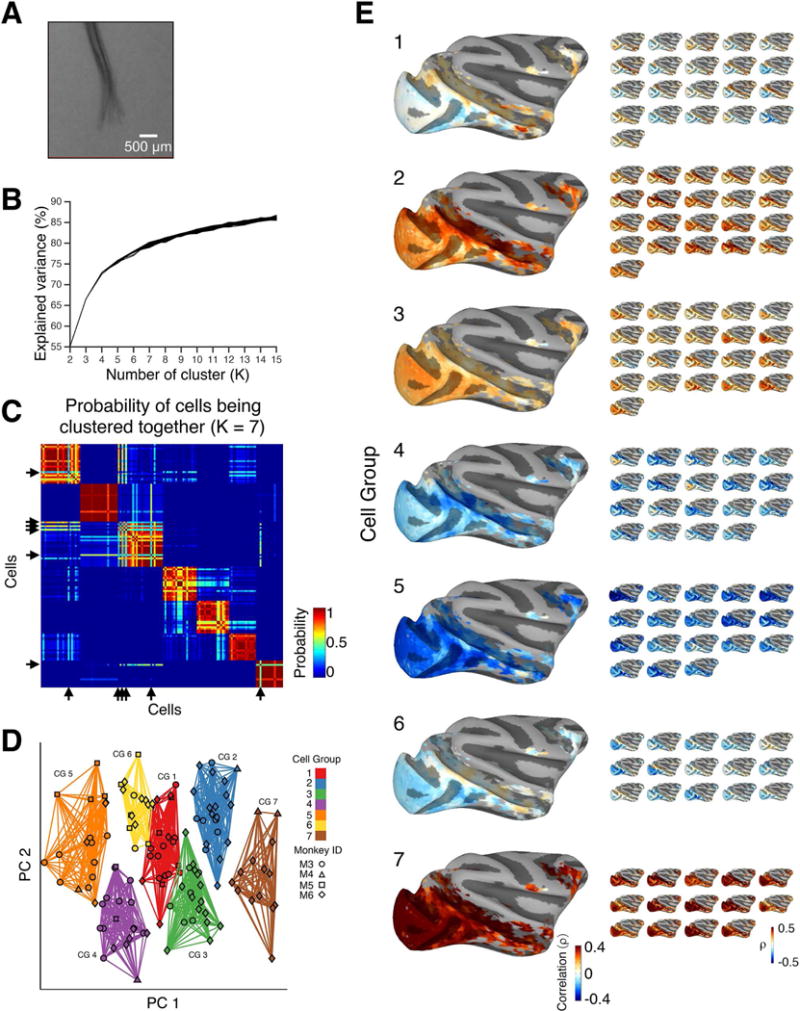
Finding subpopulation of neurons based on the single-unit functional maps using unsupervised clustering algorithms. (A) A micro-CT reconstruction of the implanted microwire bundle (reproduced from McMahon et al., 2014a). (B) Explained variance as a function of the number of clusters (K). (C) Probability of neurons being clustered together in the case of K = 7. Arrows indicate the neurons (n = 6) that were excluded due to their instability in the clustering step. (D) Result of the K-means clustering algorithm. Individual neurons (n = 129) from different monkeys (symbols) are projected onto the two-dimensional space consisting of the first and second principal components (PCs), which were computed using principal component analysis on the correlation maps (see STAR Methods and Figure S6). Results from K-means clustering (K = 7) are depicted in different colors. CG, Cell Group. (E) Functional maps for all seven Cell Groups. For each Cell Group, individual single-unit maps are averaged and shown as a Group map (larger map). Single-unit functional maps of individual neurons that belong to each group are shown as smaller maps. Note that we ordered the cell groups based on the number of neurons in each group, where Cell Group 1 - 3 had the largest number of cells (n = 21) and Cell Group 7 had the smallest (n = 14). Only voxels that were included for the clustering analysis (see STAR Methods) with sufficient stimulus-driven activity (Figure S2) are shown. See also Figure S4.

For each of the seven cell groups, we computed a group map (large brains in Figure 3E) by averaging the maps of individual neurons belonging to each group. Each group map had a characteristic pattern of correlations, which were manifest in both cortical areas (shown on flattened surfaces, Figure 4) and subcortical areas (shown on select coronal and axial slices, Figure 5). The cell groups were distinguished principally by their varied positive and negative activity correlations within face patches, motion-related cortical areas, subcortical structures, early visual areas, and frontoparietal cortical areas.

Figure 4.

Whole-brain correlation map for all Cell Groups on the flattened surface. Cortical areas correlated with each group of neurons are shown on the flattened surface. Boundaries of functionally defined face patches are superimposed (green and magenta lines). lus, lunate sulcus; ios, inferior occipital sulcus; sts, superior temporal sulcus; pmts, posterior middle temporal sulcus; amts, anterior middle temporal sulcus; ips, intraparietal sulcus; cs, central sulcus; as, arcuate sulcus; ps, principal sulcus; los, lateral orbital sulcus; mos, medial orbital sulcus. Abbreviation for face patches: PL, posterior lateral; ML, middle lateral; MF, middle fundus; AL, anterior lateral; AF, anterior fundus; AM, anterior medial; AD, anterior dorsal; PA, prefrontal arcuate; PO, prefrontal orbital face patch. Only voxels that were included for the clustering analysis (see STAR Methods) with sufficient stimulus-driven activity (Figure S2) are shown.

Figure 5.

Correlations in subcortical areas for all seven Cell Groups. Top left sagittal view indicates the location of select coronal and axial slices for (A) superior colliculus (SC) and pulvinar, (B) lateral geniculate nucleus (LGN), (C) amygdala, (D) putamen, and (E) claustrum. To focus on the subcortical correlations, voxels in cortical areas are omitted and the voxel selection criterion (Figure S2) is relaxed.

One set of neurons (Cell Group 1, n = 21 neurons), showed positive fMRI correlations that were concentrated in face patches (Figure 4A), which matches expectations based on the high level of anatomical interconnectivity between them (Grimaldi et al., 2016). The functional maps of the constituent neurons displayed some variability (see smaller maps for this group in Figure 3E), but their common component was a robust and selective association with the face patches. Among all the face patches, the anterior face patch on the STS lip (AL face patch) showed the strongest correlation (ρ = 0.32). This cell group also showed smaller negative correlation (ρ = − 0.12) with early visual cortex, particularly the peripheral regions of V1. Notably, among subcortical areas, only the medial pulvinar showed distinct and regionalized positive correlation (ρ = 0.16) with this cell group (Figure 5).

A separate set of neurons of similar size (Cell Group 2, n = 21 neurons) stood out as having strong, positive correlations (ρ = 0.41) throughout much of the STS, including both caudal, motion-related areas (MT, MST, FST) and the temporal cortex face patches (Figure 4B). Neurons in Cell Group 2 also showed strong positive correlations in LIP and arcuate sulcus. In subcortical structures (Figure 5), these cells were positively correlated with the superior colliculus, ventral portion of the pulvinar, lateral amygdala, ventral putamen, claustrum and lateral cerebellum (not shown). Positive correlations in the early visual cortex and LGN were notably weaker.

Two cell groups exhibited strong and relatively homogenous correlations throughout much of the visual cortex, which was for one group positive (Cell Group 7, n = 14 neurons, Figure 4D) and for the other negative (Cell Group 5, n = 18 neurons, Figure 4C). Aside from the polarity, the overall cortical pattern was similar for the two groups; the main difference was the absence of correlation in the face patches in Cell Group 5. Subcortical areas, including the superior colliculus, ventral pulvinar, LGN, basolateral amygdala, and ventral putamen (Figure 5) matched the broad cortical correlations in both groups. Notably, however, the claustrum differed in this regard, showing a strong positive correlation with Cell Group 7 but minimal correlation with Cell Group 5.

The remaining neurons (Cell Groups 3, 4, and 6) showed somewhat lower absolute levels of correlation that were, nonetheless, regional and distinct. Neurons in Cell Group 3 were positively correlated with much of the visual cortex (Figure 4E). This group was in that sense similar to Cell Group 7, but in this case with neurons having little or no correlation with activity in the temporal cortex face patches. Cell Group 4, on the other hand, showed negative correlations in caudal STS motion-sensitive areas, extrastriate regions in the lunate sulcus and inferior occipital sulcus, pulvinar, and superior colliculus (Figures 4F and 5). Lastly, neurons in Cell Group 6 were positively correlated with several STS regions, most notably the face patches (Figure 4G). At the same time, they were negatively correlated with broad regions of the visual cortex and minimally correlated with subcortical structures (Figure 5).

An unexpected finding was the high proportion of the visually driven correlations that were expressed across a broad swath of the visual cortex, which was present in multiple cell group maps. Applying a principal component analysis to the correlation maps, we found that approximately 80% of the map variance was carried by this broadly distributed signal (Figure S6B), which corresponds to the first principal component in Figure 3D. As the spatial distribution of these shared correlations did not match previously computed maps based on the contrast, luminance, or motion content in the movie (Russ and Leopold, 2015), the basis of this broad engagement of the visual cortex is currently unexplained.

Together, this grouping of individual cells, and the resulting correlation maps, highlight the functional diversity of neural responses within the AF face patch, suggesting that neighboring neurons participate in very different large-scale brain networks. It further suggests a possible division of labor within the local AF circuit, such that neighboring neurons exhibit distinct functional relationships with other brain areas.

Neural subpopulation matching the LFP and fMRI signals

Considering that the entire population of our single units recorded in each monkey were located within a few hundred microns of one another – within a single fMRI voxel –, the question arises as to how this single neuron activity relates to other local population measures. For example, what sort of correlation map would stem from the local field potential (LFP) signal, or the local fMRI time course itself, each of which are often taken as local population measures (Buzsáki et al., 2012)? To address these questions, we applied the same analysis as above to the high-γ (60–150 Hz) LFP signal, as well as the fMRI signal from the AF face patch.

For the LFP, we first filtered each trial’s wide-band field time-varying voltage in the gamma range and computed the band-limited power (see STAR Methods). Then, after decimating, convolving, averaging across trials, and concatenating across movies, we created fMRI maps based on these LFP signals in the same manner as with the single-unit spiking data. The resulting maps revealed a strong positive correlation that was strongest in the STS and arcuate sulcus (Figure 6A), as well as superior colliculus, ventral pulvinar, ventral putamen, lateral amygdala and claustrum (Figure S5). The pattern was similar based on the LFP signals from the three electrophysiology animals (M3, M4 and M5), although the correlation in in the lateral amygdala and claustrum was weaker in monkey M5 (Figure S5).

Figure 6.

Correlation maps of three local population signals. (A) Correlation maps based on high-γ LFP from three electrophysiology monkeys (M3, M4, and M5). (B) Correlation maps based on time series of one seed-voxel in AF face patch from two fMRI monkeys (M1 and M2). (C) Correlation map based on the averaged spiking activity of the population of neurons (n = 129) recorded from the four electrophysiology monkeys. All maps are plotted on the brain of Monkey M1 except the seed-voxel map of Monkey M2 in (B). Only voxels with sufficient stimulus-driven activity (Figure S2) are shown. See also Figure S5.

For the fMRI mapping, we took a single voxel within the AF region and applied the same whole-brain mapping procedure (Figure 6B, see STAR Methods). The maps were again marked by a strong positive correlation in the STS and arcuate sulcus, as well as in the same subcortical structures observed in the LFP mapping (Figure S5).

In comparing the maps computed from the local LFP and fMRI signals to those derived from the individual neurons, it was evident that one of the cell groups was very similar. Namely, Cell Group 2 (Figure 3E and 4B, Figure S5) showed the strongest correlations in the STS, arcuate, and subcortical regions that closely matched the spatial correlation patterns observed in the LFP and fMRI seed maps. None of the other cell groups bore such similarity. Moreover, we also examined the grand mean average spiking activity across the AF population. For this average spiking time course map (Figure 6C), the pattern of correlations did not match either the LFP or the fMRI maps, though it did show a notably high level of correlation within the face patches themselves. In summary, based on this mapping method, the locally measured fMRI and high-γ LFP activity in the AF face patch was reflected in the spiking of one particular cell subpopulation, which corresponded to approximately 16% of the single units we recorded.

Discussion

In the present study, we exploited the coverage of fMRI to investigate the functional diversity of neural responses within a cubic millimeter of the cerebral cortex. Our central finding is that neurons intermingled within a tiny cortical volume are affiliated in very different ways with activity throughout the brain. This functional diversity could be summarized by arranging cells into functional groups based on their map of correlation with fMRI signals across the brain. The map derived from only one of these groups, composed of ~16% of neurons we recorded, resembled the mapping based on locally measured fMRI and LFP signals. By classifying neural function based on whole-brain correlation, rather than feature selectivity, this approach offers a new and alternative perspective on thinking about diversity within a local neural population.

Possible origins of response diversity within a cortical microcircuit

During the viewing of natural videos, neighboring neurons within the AF population differed considerably in their response time courses and their correspondence with activity in other brain areas. Given the proximity of the cells involved, what physiological factors might contribute to this response independence? One possibility is that the construction of the cortical microcircuit, through its local interconnections, promotes activity independence, or decorrelation, among individual cells.

Another interesting possibility, not mutually exclusive, is that neighboring neurons are independently but effectively innervated by sparse, long-range axonal afferents. Pyramidal neurons in the cerebral cortex, including those in face patches (Grimaldi et al., 2016), receive a diversity of long-range inputs. Previous work in mice has shown that the selective synaptic innervation of local neurons can cause neighboring neurons to abruptly depart from an otherwise synchronous state and exhibit distinct patterns of spiking (Poulet and Petersen, 2008; for review, see Petersen and Crochet, 2013).

It is attractive to consider the observed coupling of individual neurons with specific brain networks as a consequence of selective long-range inputs. However, it must be emphasized that this interpretation is highly speculative, and that the observed correlations cannot and should not be taken as a measure of anatomical or functional connectivity. Indeed, extrapolating from anatomical connections alone (Grimaldi et al., 2016), one might expect a high degree of exclusive correlation with the face-patch network for all AF subpopulations. Yet we observed that only one subpopulation (Cell Group 1) followed the predictions set by the known anatomical connections. Most of the correlation we observed showed more broadly distributed correlated and anti-correlated responses, for example with STS motion areas and early retinotopic areas. Interpreting these findings with respect to any particular anatomical connections is challenging and unlikely to be fruitful.

It is important to mention that the level of functional diversity in a given location may vary strongly across the cortex. The microwire bundles in the present study were submillimeter in their distribution, but the localization relative to the center or margins of a face patch are more approximate than that. In the ML face patch, for example, the level of response homogeneity to flashed images varies systematically as a function of the distance from face patch center (Aparicio et al., 2016). In our AF recordings, the level of observed functional diversity was similar across animals despite necessarily different electrode bundle locations. Future work aims to understand the extent to which the high level of local diversity observed in the present study varies across functionally specialized areas.

Implications for functional MRI mapping

While this study did not aim to investigate neurovascular coupling, its basic findings do have some potential implications for linking fMRI to electrophysiological responses. The neural recordings in the present study were conducted within a space less than the size of a single voxel in each animal. One surprising finding was that traditional measures of population activity, including the local fMRI and high-γ LFP time courses, produced whole-brain maps that closely matched only one of the identified neuronal subpopulations (Cell Group 2; representing just 16% of all neurons). Thus it would appear that certain neural subpopulations have a stronger role than others in shaping local fMRI and LFP population measures. More work is needed to understand this link and its interdependence with stimulus feature selectivity and underlying functional anatomy.

The present findings do raise a somewhat daunting prospect for the investigation of the brain using fMRI, a technique that depends on some measure of functional localization. Namely, if the neural contents of a given fMRI voxel are strongly heterogeneous, and composed of multiple functional subpopulations, how does one interpret fMRI signals derived from a single location in the brain? The other side of this issue relates to the spatial contiguity of functionally homogeneous neurons. Ongoing work will determine whether the diversity of fMRI correlation maps encountered in AF are similar to those encountered elsewhere, as in other face patches. If the distribution is similar, one outcome might be that functional processing modules are not cleanly segregated between the patches. Instead, circuits devoted to particular aspects of processing might be distributed across multiple patches, and then within each patch they might be intermingled with neural populations that are focused on a different set of features. The face patch domains may thus indicate the common denominator of face processing, but may not represent a set of processing stages or hierarchy with spatially segregated nodes. If true, fMRI approaches may need to further adapt to deemphasize the traditional assumptions of functional localization, a trend that in some ways resonates with modern multivariate fMRI analysis approaches (Kriegeskorte and Kievit, 2013).

Trade-offs in naturalistic, data-driven approaches to study high-level vision

The field of visual neuroscience is founded on experiments carefully designed to restrict a known stimulus to a well-defined region of the retina, and to then ask which critical stimulus features drive neuronal activity. The current study is a departure from this mode of investigation, both in its use of naturalistic stimuli and in its combination of single unit and fMRI methods. Most importantly, we approached single-cell responses of visual neurons not by probing their feature spaces, but instead by probing their activity covariation across widely studied regions of the brain. This paradigm, like any, carries with it a number of experimental trade-offs.

With respect to naturalistic stimuli, the weaknesses and strengths are in some ways the same: the complexity of the videos and the freedom of the animal to explore its features. The free viewing of dynamic videos does not lend itself well to strict hypothesis testing of stimulus features. It does, however, tap into the response diversity of neurons by presenting a rich spatiotemporal content of stimulation not typically encountered in more traditional paradigms. The level of tolerance for stimulus details, as well as eye behavior of the subject, may make naturalistic stimuli most appropriate for studying high-level sensory areas. An additional benefit of naturalistic paradigms is that they lend themselves to translational work — non-human primates and humans, including a range of patient groups, are readily engaged by naturalistic videos (Berg et al., 2009; Hasson et al., 2004). In the present study, the single-unit-to-fMRI approach was robust even though the two measures were obtained from different subjects, suggesting that it will extend across species. This introduces a translational opportunity to relate single-unit activity from non-human primate models to fMRI signals that can be readily acquired in humans, in both typical and atypical populations.

The trade-offs surrounding the correlational mapping approach are not yet completely clear, as the method is new and requires more exploration. On the one positive side, the method provides a new perspective on local cell populations based on whole-brain activity relationships, rather than on features. This aspect of the experimental design can be liberating, as it allows one to tap into the richness and complexity of visual stimuli to which the brain is naturally accustomed. The strong segregation of neural subpopulations based on this method was surprising and raises questions about the types of neural mechanisms that might give rise to the specific correlational patterns, as discussed above. On the other hand, the negative aspect of this approach is a loss of control over the precise features that are responsible for the neurons’ consistent responses across trials. The specific stimulus features that give rise to the responses are clearly important, and serve as the basis for the vast majority of previous studies of the inferior temporal cortex. However, exploring this aspect of the neural responses requires considerable additional effort. Despite marked consistency in both the spiking time courses and the whole brain mapping of individual neurons, the underlying “feature selectivity” often remained opaque. It is important to state, however, that any feature-based theory of inferotemporal function is only as valuable as its capacity to explain neural responses during natural vision. One particular surprise in this data set, which has prompted further investigation, is the extent to which neurons described categorically as “face cells” are responsive to other features, and in their responses correlated with activity throughout many parts of the brain that are not specialized for faces. The existence of such neurons, amid multiple intermixed groups populating a face patch, is a finding that is a direct consequence of the approach taken here. Furthermore, the very high proportion of the variance explained by correlation over a large swath of visual cortex (Figure S6) raises new questions about the types of visual information that face patch neurons respond to under natural conditions. Understanding feature processing as it pertains to natural vision, and making the link to the known selectivity using more conventional stimuli, will likely require a back and forth between the presentation of isolated, parameterized stimuli and more naturalistic, but uncontrolled stimuli. One interpretation of this broad activation is that it may relate to the unspecific activation of object stimuli throughout the visual cortex, such as when object activation is contrasted with responses to a blank screen. However, this interpretation is not straightforward, since the paradigm differs from most category mapping experiments, and a similarly broad visual activation would be expected from any rich visual stimulus, including faces.

Another interesting opportunity for single-unit mapping, which was not studied here, is the explicit separation of stimulus-driven versus trial-specific covariation. In the present study, the determination of single-unit fMRI maps was greatly aided by the capacity to average both single unit and fMRI responses across multiple sessions. This capacity increased the signal-to-noise ratio and allowed us to focus on the consistent, stimulus-driven covariation. However, the analysis of trial-specific fluctuations is also a topic of great interest, as it can tap into the brain’s cognitive and behavioral states that are otherwise averaged out across trials. To investigate the moment-to-moment brain activity that is not strictly driven by repeated presentations of a stimulus, it is necessary to collect measures of interest in parallel. For example, in a previous study, we analyzed fMRI data with respect to the moment-by-moment eye gaze behavior (Russ et al. 2016). Extending this type of approach to the relationship between single units and fMRI requires simultaneous recordings in the fMRI scanner, which is now readily achievable (Godlove et al., Society for Neuroscience Annual Meeting Abstr., 2015). Under such conditions, it is possible to study not only the correspondence between visually driven components of brain activity, but also those that fluctuate less predictably, such as those related to attention, memory, and other cognitive factors. In summary, despite the challenges inherent in the naturalistic, data-driven paradigm described here, these departures from a simple stimulus-to-brain mapping present new opportunities for examining the functional networks engaged during natural vision.

Taken together, our findings illustrate the power of data-driven approaches to investigate the relationship between local circuit complexity and responses measured throughout the brain. Hypotheses stemming from such approaches can be tested using more conventional and systematic testing with precise control over stimulus features. For such testing, longitudinal single-unit recordings are particularly well suited, as they permit the study of the same, individual neurons using both naturalistic (data-driven) and conventional (designed) paradigms. The combination of these methods will be essential for understanding the nature of functional specialization and its instantiation in high-level vision.

STAR Methods

CONTACT FOR REAGENT AND RESOURCE SHARING

Further information and requests for resources should be directed to and will be fulfilled by the Lead Contact, Soo Hyun Park (soohyun.park@nih.gov).

EXPERIMENTAL MODEL AND SUBJECT DETAILS

Two adult rhesus macaque monkeys participated in the fMRI study (monkeys M1 and M2; females, both 6 years old, 7.1 and 7.0 kg), and four adult rhesus monkeys participated in electrophysiological recordings (monkeys M3 (female, 6 years old, 5.6 kg), M4 (male, 8 years old, 8.7 kg), M5 (female, 9 years old, 5.0 kg), and M6 (female, 14 years old, 7.3 kg). All monkeys were implanted with a custom-designed and fabricated fiberglass headpost, which was used to immobilize the head during experiments. The four electrophysiology monkeys were implanted with chronic microwire electrode bundles in the AF face patch, which was functionally localized using a standard fMRI block design. All procedures were approved by the Animal Care and Use Committee of the US National Institutes of Health (National Institute of Mental Health) and followed US National Institutes of Health guidelines.

METHOD DETAILS

The electrophysiological and the fMRI responses analyzed in the present study were recorded separately using two independent groups of animals. A full description of each set of methods, including surgical procedures, tasks, and behaviors, is given in previous publications that detail electrophysiology (McMahon et al., 2015) and fMRI investigations (Russ and Leopold, 2015) that generated most of the movie-driven datasets studied here. Additionally, refer to previous work (McMahon et al., 2014a; McMahon et al., 2014b) for the technical details of longitudinal single-unit recordings using chronic microwire bundles and their targeted implantation in the face patch.

Visual Stimulus Presentation

We used three 5-min videos depicting macaque monkeys engaged in a range of natural behaviors, including interactions with other macaques as well as humans. The videos used in the current study consisted of scenes taken from commercially available nature documentaries and were a subset of movies generated and used in the previous studies (McMahon et al., 2015; Russ and Leopold, 2015). Videos were in 640 × 480 pixel resolution with a frame rate of 30 frames per second. For both fMRI and electrophysiology, the monkeys sat upright in a specially designed primate chair and watched the movies on the screen with their head stabilized by a head post. Movies were displayed using the Psychophysics Toolbox (Brainard, 1997) running on a separate PC. All aspects of the task related to timing of stimulus presentation, eye-position monitoring, and reward delivery were controlled by custom software courtesy of David Sheinberg (Brown University, Providence, RI) running on a QNX computer.

Experimental Design

fMRI

Subjects viewed the visual stimuli projected onto a screen above their head through a mirror. Horizontal and vertical eye positions were recorded using an MR-compatible infrared camera (MRC Systems, Heidelberg, Germany) fed into an eye tracking system (SensoMotoric Instruments GmbH, Teltow, Germany) at the sampling rate of 200 Hz. Prior to the experimental sessions, subjects were trained on a fixation task with a 0.2°– 0.5° white dot to permit calibration of the eye signal. Each session started with an eye calibration task and the calibration was repeated every second trial of 5-min movie watching. Each 5-min trial began with a 500 ms presentation of a white central point surrounded by a 10° diameter annulus, the extent of which indicated the tolerance window of gaze positions for reward. The size of the movies on the screen was of 10° wide and 8° high. Since the annulus was approximately as large as the stimulus itself, subjects were free to direct their gaze to the content of the video and received a drop of juice reward every 2 s if their eyes were within the movie frame. Subject M1 and M2 watched each of the three movies 28 – 36 and 29 – 40 times, respectively. The animals’ eye movements are within-screen for the majority (> 80%) of the movie presentation.

In separate sessions, we localized face patches using a block design with alternating blocks of either monkey faces (Gothard et al., 2004) or phase scrambled versions of those faces. Localization runs consisted of eight 48s-blocks. Within a block, each 12° image appeared for 2 s. Subjects were free to scan the images, and were rewarded every 2 s if their gaze was within the frame of the image (6°-radius “fixation window”). Each subject participated in multiple face localizer runs (17 in M2, 37 in M1).

Electrophysiology

Subjects viewed the movies on an LCD monitor, where movies were presented within a rectangular frame of 10.4° wide and 7.6° high. Horizontal and vertical eye positions were recorded using an infrared video-tracking system (EyeLink; SR Research). Eye position was calibrated at the beginning of each session and as needed during subsequent inter-trial intervals. One monkey (M3) viewed the movie without liquid reward, whereas the other three (M4, M5 and M6) received a water or juice reward for directing gaze to the movie, defined as a large “fixation window” of 10.5°. Subject M3, M4, M5, and M6 watched each of the three movies for 3– 11, 13 – 15, 8, and 11 times, respectively.

Data acquisition

fMRI Scanning

Structural and functional images were acquired in a 4.7-T, 60-cm vertical scanner (Bruker Biospec, Ettlingen, Germany) equipped with a Bruker S380 gradient coil. We collected whole brain images with an eight-channel transmit and receive radiofrequency coil system (Rapid MR International, Columbus, OH). Functional echo planar imaging (EPI) scans were collected as 40 sagittal slices covering the whole brain with an in-plane resolution of 1.5 mm × 1.5 mm and a slice thickness of 1.5 mm. Repetition time and echo time were 2.4 s and 12 ms, respectively. Either 125 or 250 whole brain images were collected for each 5-min presentation of one video, corresponding to 5 or 10 min scans. The 10 min scans contained an additional 2.5 min of rest (blank screen) at both the beginning and end of the scan. Monocrystalline iron oxide nanoparticles (MION), a T2* contrast agent, was administered prior to the start of EPI data acquisition. MION doses were determined independently for each subject to attain a consistent drop in the signal intensity of approximately 60% (Leite et al., 2002), which corresponded to ~ 8 – 10 mg/kg. Subjects participated in up to twelve 5-min trials per scanning session.

Electrophysiological Recordings

Electrophysiological recordings were obtained from bundles of 32 NiCr or 64 NiCr microwires chronically implanted in the AF face patch (McMahon et al., 2014a). The microwire electrodes were designed and initially constructed by Dr. Igor Bondar (Institute of Higher Nervous Activity and Neurophysiology, Moscow, Russia) and subsequently manufactured commercially (Microprobe). Data were collected using either a Multichannel Acquisition Processor with 32-channel capacity (Plexon) or an RS4 (or RZ2 in case of recordings in monkey M6) BioAmp Processor with 128-channel capacity (Tucker-Davis Technologies). Broadband electrophysiological responses were collected, which allowed for post-hoc filtering of spikes and local field potentials (LFPs).

QUANTIFICATION AND STATISTICAL ANALYSIS

Preprocessing

fMRI

All fMRI data were analyzed using the AFNI/SUMA software package (Cox, 1996) and custom-written MATLAB code (MathWorks, Natick, MA). Raw images were first converted into AFNI data file format. Slice timing was corrected to be alternating in the z+ direction using the AFNI function 3dTshift with an option of using the quintic (5^th order) Lagrange polynomial interpolation. Motion correction algorithms were applied to each EPI time course using the AFNI function 3dvolreg, followed by correction for static magnetic field inhomogeneity using the PLACE algorithm (Xiang and Ye, 2007). Each session was then registered to a template session, allowing for the combination of data across multiple testing days. Before combining the data across multiple days, we converted each 5-min scan into the percent signal change by subtracting the mean and then dividing by the mean.

For the face-localizer sessions, functional maps were produced for each monkey by concatenating all face-localizer runs and computing the response contrast (t-value) between the two stimulus conditions. Face patch ROIs were created for the individual face patches by selecting all voxels above a threshold of t = 5 (t = 2 for prefrontal patches). These ROIs were subsequently projected to the flattened surface and the boundary for each face patch was drawn on the surface (Figure 2 and Figure 5).

Electrophysiology

Individual spikes and LFPs were extracted off-line from the same broadband signal by band-pass filtering between 300 and 5000 Hz for spikes and by low-pass filtering at 300 Hz for LFP, using a second-order Butterworth filter and the MATLAB function filtfilt.m. Spikes were sorted using the OfflineSorter software package (Plexon) or Wave_clus spike-sorting package (Quiroga, et al., 2004). We identified single units longitudinally across days based on multiple criteria, including the similarity in waveform shapes, similarity in interspike interval histograms across days, and the distinctive visual response pattern generated by isolated spikes as a neural “fingerprint,” which we previously found in this area of cortex. Further details on spike sorting and longitudinal identification of neurons across days can be found in here (Bondar et al., 2009; McMahon et al., 2014a).

For three of the four electrophysiology monkeys, the LFP signal was filtered into four non-overlapping frequency bands: 4 – 12, 12 – 25, 40 – 60, and 60 – 150 Hz. We then created band-limited power (BLP) signals by rectifying each band-limited single-trial response. After determining that the low-frequency signals recorded on different wires were largely redundant (median cross-channel correlation coefficient, r = 0.97), we took the traces from a single channel as the representative LFP.

Functional maps derived from single units

For each individual neuron in AF, we computed whole-brain functional maps by correlating the movie-driven signals from the two methods (fMRI and electrophysiological recording), where the value of each voxel was the correlation coefficient between its fMRI time course and the single AF neuron’s time course (Figure 1C). This computation involved several preprocessing steps that permitted the two signals to be directly correlated. For single-unit time course, we first down-sampled each single-unit response to match the fMRI temporal resolution by taking the sum of spikes in bins of 2.4 s, which was the fMRI sampling interval (i.e. repetition time). The down-sampled time series were then averaged across trials for a given 5-minute movie (Figure 1A, step 1). Second, we convolved a generic hemodynamic impulse response function (gamma probability density function) to the averaged, normalized (i.e. centered to the mean) time course to match the hemodynamic delay of MION responses (Figure 1A, step 2). These two pre-processing steps on the single-unit data enabled a direct comparison between the neuronal and fMRI measurements. We then concatenated the convolved neuronal time courses from the three different movies, resulting in a single 15-minute time series for each cell. For fMRI responses, we first averaged the time series across all trials for each movie (Figure 1B, step 1). The possible linear trend in the averaged time series was removed using the detrend.m function in MATLAB. The first seven TRs (16.8 s) of each movie were excluded to eliminate the hemodynamic onset response associated with the initial presentation of each video. Time-series data were then concatenated across three movies, resulting in 15-min (i.e. 375 volumes) time series of each voxel in the whole brain (Figure 1B, step 2). After this preparation of the time courses, for each single unit we computed the Spearman’s rank correlation coefficients between the neuronal time course and fMRI time courses of all the voxels in the whole brain (Figure 1C). The resulting correlation maps were not critically dependent on the exact hemodynamic impulse response function, when we used three different functions including two from the previous literature (Leite et al., 2002; Silva et al., 2007).

With respect to reproducibility within subjects, we performed a split-half analysis to assess the reproducibility of the patterns of correlations for a given neuron. Specifically, for a given neuron, we randomly chose half of the total trials, averaged time courses across those trials, computed a whole-brain correlation map, then compared two maps from each half of the trials. To assess the similarity of the maps, we computed Spearman’s correlations between two maps, i.e. two vectors (n = 15, 495) of correlation. The median correlation across neurons (n = 135) was 0.93.

Except for the maps shown in Figure 2A–2B and Figure S1, we applied a mask to exclude the voxels that failed to respond consistently to the movie content. The exclusion criterion was based on the absolute magnitude of the fMRI signal averaged across many trials. Specifically, for each voxel, we took the absolute value of the 15-min time series averaged over 28 – 40 trials (Figure 1B), and then computed the average of that absolute magnitude over time. The distribution of the absolute movie-driven response magnitude was highly skewed with a heavy tail, and ranged from 0.3 % to 3.6 % with a median of 1.09 % (Figure S2A). We used the median as the minimum threshold for defining voxels that were sufficiently responsive to the movies. To make a mask, we applied Gaussian smoothing on movie-driven response magnitude maps (using the smooth3.m function in MATLAB) and selected for further analysis only voxels with magnitude above 1.09 % (Figure S2B). In subsequent analyses, we applied this mask to the whole-brain correlation maps.

Significance testing of the correlation coefficients

To determine the level of correlation between a voxel and a non-stimulus related noise with similar statistics to each neuron that could remain after averaging across multiple trials, we used a bootstrap method to compute the 95% confidence interval of correlation values for each voxel and single unit. Specifically, we performed a resampling procedure called stationary bootstrap (Politis and Romano, 1994) using the stationaryBB.m function available from MathWorks File Exchange (https://www.mathworks.com/matlabcentral/fileexchange/53701-bootstrapping-time-series?focused=5590575&tab=function), where new bootstrap samples of the single unit time course were generated by sampling blocks of the time series, randomly with replacement from the original spike count time series. The length of each resampling block was randomly chosen from a geometric distribution with a mean of 1 s (i.e. 10 data points of spike counts in 100-ms bins). In each bootstrapping, we generated a resampled single unit time series, convolved with a hemodynamic impulse response function, and computed Spearman’s rho with the set of original voxel time courses from the whole brain. We repeated this procedure 1,000 times to obtain a distribution of 1,000 correlation coefficients for each voxel, from which we computed the 95% confidence intervals. The low and high boundary of the intervals were −0.1904 and 0.1890, respectively, when averaged across voxels and then across cells.

Clustering of single units

To find functional subgroups of neurons based on their correlation pattern with other brain areas, we applied a k-means clustering algorithm on the matrix of correlation values between neurons and voxels, using the kmeans.m function in MATLAB’s Statistics Toolbox with the squared Euclidean distance metric. We limited this analysis to the voxels that showed an absolute correlation value larger than 0.3 with at least six neurons, which corresponded to 5% of the population. 5,581 voxels from the whole brain passed this criterion and were used for clustering of the neurons (n = 135) from the four electrophysiology monkeys.

Since K-means clustering is not a deterministic algorithm, we repeated the clustering procedure 100 times each for K values ranging from 2 to 15, and for each repetition for each K, we computed the percentage of variance explained by the clustering (i.e., the between-clusters sum-of-squares relative to the total sum-of-squares) (thin lines in Figure 3B). There were asymptotic increases as the K value increased, but no clear point of concavity. When we compute the difference, or increase in explained variance that we gain as we increase the number of clusters (i.e. first derivative of the curve in Figure 3B), we found that there was no increase from K = 7 to K = 8 in most repetitions. Further, through the 100 repetitions of the same procedure, we could assess the stability of the clustering by computing the probability of each cell being clustered with other cells (Figure 3C). This probability measure further provided us useful information on determining the number of clusters: we found that the stability of clustering varied substantially depending on the K (Figure S4A). Based on 1) the gain we can get in the explained variance as we increase the K (Figure 3B) and 2) the stability of the clustering (Figure 3C), we determined that seven clusters, which corresponds to seven cell groups, were adequate to summarize this population of neurons with high stability (see Figure S4A for clustering results using different Ks). After we determined the number of clusters, if a neuron failed to be clustered in any cluster 50% of the time, that neuron was excluded from the subsequent analysis of averaging maps within the cluster. According to this criterion, we excluded six neurons (Figure 3C, arrows).

To verify the clustering results from K-means, we used principal component analysis on the matrix of correlation values between neurons and voxels (135 × 5,581) (using the pca.m function in the MATLAB Statistics Toolbox with default options). The first four principal components, each of which explained more than 3% of the total map variance (79.7%, 6.8%, 5.3%, and 3.3%, respectively; Figure S6), together explained 95% of the total map variance. We then plotted the scores of the first two principal components for each neuron (Figure 3D). Note that the six neurons that are excluded above were not plotted in Figure 3D.

We also evaluated clustering results using signals other than the fMRI correlation maps. We applied the same K-means algorithm to matrices with four different kind of signals (Figure S4B): 1) neuronal time series at a relatively high temporal resolution (10 Hz), computed by taking the sum of spikes in 100 ms bins. 2) normalized (z-scored) 10Hz neuronal time series described in 1). 3) non-normalized neuronal time series at the fMRI sampling resolution, computed by taking the sum of spikes in 2.4 s bins. 4) neuronal time series at the fMRI sampling resolution reflecting hemodynamic delay, computed by convolving the generic hemodynamic function to the time series described in 3). Note that this fourth time series was used to create the whole-brain correlation maps. We also repeated the K-means clustering on each of these four values while varying K values, and the results when K = 7 are shown in Figure S4B.

Functional maps derived from other time series

We computed three types of functional maps in addition to the whole-brain maps from each single unit. First, using an approach similar to that devised for single units, we created functional maps from the LFP signal (Figure 6A), which was recorded simultaneously with spike activity from the AF face patch of three animals (M3, M4, and M5). We first divided the wide-band LFP signal into four different frequency bands and computed the BLP signals for each band (see Preprocessing: electrophysiology). Then, we computed the z-score of the raw BLP signal for each viewing. Next, we matched the temporal resolution of BLP signals to fMRI signals as we did for each spiking time series, by averaging the BLP for every TR duration (i.e. 2.4 s). Finally, we averaged across trials for a given 5-minute movie and concatenated time courses from the three different movies, resulting in a single 15-minute time series for each frequency band. After that, we computed voxel-wise correlations between the BLP in each frequency and the fMRI signals. Second, we generated AF seed-voxel correlation maps (Figure 6B), using one randomly chosen voxel from the functionally defined AF face patch of the two fMRI animals (M1 and M2) as the seed. After initial preprocessing, which included averaging across trials and concatenating time courses from the three movies, we computed voxel-wise correlations between the time course of the seed-voxel and all the voxels from the whole brain. Resulting maps remained the same whether we used other individual voxels within AF, or the averaged response time course from the AF ROI. Third, we made a mean neuronal response map (Figure 6C). For this, we averaged the response time courses across all neurons from four monkeys (M3, M4, M5, and M6) (n = 129), after initial preprocessing, which included averaging across trials and concatenating time courses from the three movies. We then computed voxel-wise correlations between the averaged neuronal time series and all the voxels from the whole brain.

DATA AND SOFTWARE AVAILABILITY

Analysis-specific code and data are available by request to the Lead Contact.

Highlights.

• We compared responses of macaque face patch cells to fMRI activity across the brain

• Single neurons yielded diverse fMRI correlation maps in response to natural videos

• Maps generated by single units within < 1mm³ in the AF face patch differed greatly

• Clustering neurons based on such maps revealed functional subpopulations within AF

References

- Aparicio PL, Issa EB, DiCarlo JJ. Neurophysiological Organization of the Middle Face Patch in Macaque Inferior Temporal Cortex. J Neurosci. 2016;36:12729–12745. doi: 10.1523/JNEUROSCI.0237-16.2016. [DOI] [PMC free article] [PubMed] [Google Scholar]
- Bartels A, Zeki S. Brain dynamics during natural viewing conditions—a new guide for mapping connectivity in vivo. Neuroimage. 2005;24:339–349. doi: 10.1016/j.neuroimage.2004.08.044. [DOI] [PubMed] [Google Scholar]
- Bell AH, Malecek NJ, Morin EL, Hadj-Bouziane F, Tootell RBH, Ungerleider LG. Relationship between functional magnetic resonance imaging-identified regions and neuronal category selectivity. J Neurosci. 2011;31:12229–12240. doi: 10.1523/JNEUROSCI.5865-10.2011. [DOI] [PMC free article] [PubMed] [Google Scholar]
- Berg DJ, Boehnke SE, Marino RA, Munoz DP, Itti L. Free viewing of dynamic stimuli by humans and monkeys. J Vis. 2009;9:19–19. doi: 10.1167/9.5.19. [DOI] [PubMed] [Google Scholar]
- Bondar IV, Leopold DA, Richmond BJ, Victor JD, Logothetis NK. Long-term stability of visual pattern selective responses of monkey temporal lobe neurons. PLoS ONE. 2009;4:e8222. doi: 10.1371/journal.pone.0008222. [DOI] [PMC free article] [PubMed] [Google Scholar]
- Brainard DH. The psychophysics toolbox. Spat Vis. 1997;10:433–436. [PubMed] [Google Scholar]
- Buzsáki G, Anastassiou CA, Koch C. The origin of extracellular fields and currents–EEG, ECoG, LFP and spikes. Nat Rev Neurosci. 2012;13:407–420. doi: 10.1038/nrn3241. [DOI] [PMC free article] [PubMed] [Google Scholar]
- Cox RW. AFNI: software for analysis and visualization of functional magnetic resonance neuroimages. Comput Biomed Res. 1996;29:162–173. doi: 10.1006/cbmr.1996.0014. [DOI] [PubMed] [Google Scholar]
- Crochet S, Poulet JFA, Kremer Y, Petersen CCH. Synaptic mechanisms underlying sparse coding of active touch. Neuron. 2011;69:1160–1175. doi: 10.1016/j.neuron.2011.02.022. [DOI] [PubMed] [Google Scholar]
- Douglas RJ, Martin KA. Neuronal circuits of the neocortex. Annu Rev Neurosci. 2004;27:419–451. doi: 10.1146/annurev.neuro.27.070203.144152. [DOI] [PubMed] [Google Scholar]
- Freiwald WA, Tsao DY, Livingstone MS. A face feature space in the macaque temporal lobe. Nat Neurosci. 2009;12:1187–1196. doi: 10.1038/nn.2363. [DOI] [PMC free article] [PubMed] [Google Scholar]
- Gothard KM, Erickson CA, Amaral DG. How do rhesus monkeys (Macaca mulatta) scan faces in a visual paired comparison task? Anim Cogn. 2004;7:25–36. doi: 10.1007/s10071-003-0179-6. [DOI] [PubMed] [Google Scholar]
- Grimaldi P, Saleem Kadharbatcha S, Tsao D. Anatomical Connections of the Functionally Defined “Face Patches” in the Macaque Monkey. Neuron. 2016;90:1325–1342. doi: 10.1016/j.neuron.2016.05.009. [DOI] [PMC free article] [PubMed] [Google Scholar]
- Hasselmo ME, Rolls ET, Baylis GC. The role of expression and identity in the face-selective responses of neurons in the temporal visual cortex of the monkey. Behav Brain Res. 1989;32:203–218. doi: 10.1016/s0166-4328(89)80054-3. [DOI] [PubMed] [Google Scholar]
- Hasson U, Malach R, Heeger DJ. Reliability of cortical activity during natural stimulation. Trends Cogn Sci. 2010;14:40–48. doi: 10.1016/j.tics.2009.10.011. [DOI] [PMC free article] [PubMed] [Google Scholar]
- Hasson U, Nir Y, Levy I, Fuhrmann G, Malach R. Intersubject synchronization of cortical activity during natural vision. Science. 2004;303:1634–1640. doi: 10.1126/science.1089506. [DOI] [PubMed] [Google Scholar]
- Hung C-c, Yen CC, Ciuchta JL, Papoti D, Bock NA, Leopold DA, Silva AC. Functional mapping of face-selective regions in the extrastriate visual cortex of the marmoset. J Neurosci. 2015;35:1160–1172. doi: 10.1523/JNEUROSCI.2659-14.2015. [DOI] [PMC free article] [PubMed] [Google Scholar]
- Huth AG, Nishimoto S, Vu AT, Gallant JL. A continuous semantic space describes the representation of thousands of object and action categories across the human brain. Neuron. 2012;76:1210–1224. doi: 10.1016/j.neuron.2012.10.014. [DOI] [PMC free article] [PubMed] [Google Scholar]
- Issa EB, DiCarlo JJ. Precedence of the eye region in neural processing of faces. J Neurosci. 2012;32:16666–16682. doi: 10.1523/JNEUROSCI.2391-12.2012. [DOI] [PMC free article] [PubMed] [Google Scholar]
- Issa EB, Papanastassiou AM, DiCarlo JJ. Large-scale, high-resolution neurophysiological maps underlying FMRI of macaque temporal lobe. J Neurosci. 2013;33:15207–15219. doi: 10.1523/JNEUROSCI.1248-13.2013. [DOI] [PMC free article] [PubMed] [Google Scholar]
- Kanwisher N, McDermott J, Chun MM. The fusiform face area: a module in human extrastriate cortex specialized for face perception. J Neurosci. 1997;17:4302–4311. doi: 10.1523/JNEUROSCI.17-11-04302.1997. [DOI] [PMC free article] [PubMed] [Google Scholar]
- Kriegeskorte N, Kievit RA. Representational geometry: integrating cognition, computation, and the brain. Trends Cogn Sci. 2013;17:401–412. doi: 10.1016/j.tics.2013.06.007. [DOI] [PMC free article] [PubMed] [Google Scholar]
- Leite FP, Tsao D, Vanduffel W, Fize D, Sasaki Y, Wald LL, Dale AM, Kwong KK, Orban GA, Rosen BR. Repeated fMRI using iron oxide contrast agent in awake, behaving macaques at 3 Tesla. Neuroimage. 2002;16:283–294. doi: 10.1006/nimg.2002.1110. [DOI] [PubMed] [Google Scholar]
- Leopold DA, Bondar IV, Giese MA. Norm-based face encoding by single neurons in the monkey inferotemporal cortex. Nature. 2006;442:572–575. doi: 10.1038/nature04951. [DOI] [PubMed] [Google Scholar]
- Mantini D, Corbetta M, Romani GL, Orban GA, Vanduffel W. Data-driven analysis of analogous brain networks in monkeys and humans during natural vision. NeuroImage. 2012;63:1107–1118. doi: 10.1016/j.neuroimage.2012.08.042. [DOI] [PMC free article] [PubMed] [Google Scholar]
- McMahon DBT, Bondar IV, Afuwape OAT, Ide DC, Leopold DA. One month in the life of a neuron: longitudinal single unit electrophysiology in the monkey visual system. J Neurophysiol. 2014a;112(7):1748–1762. doi: 10.1152/jn.00052.2014. [DOI] [PMC free article] [PubMed] [Google Scholar]
- McMahon DBT, Jones AP, Bondar IV, Leopold DA. Face-selective neurons maintain consistent visual responses across months. Proc Natl Acad Sci USA. 2014b;111(22):8251–8256. doi: 10.1073/pnas.1318331111. [DOI] [PMC free article] [PubMed] [Google Scholar]
- McMahon DBT, Russ BE, Elnaiem HD, Kurnikova AI, Leopold DA. Single-Unit Activity during Natural Vision: Diversity, Consistency, and Spatial Sensitivity among AF Face Patch Neurons. J Neurosci. 2015;35:5537–5548. doi: 10.1523/JNEUROSCI.3825-14.2015. [DOI] [PMC free article] [PubMed] [Google Scholar]
- Moeller S, Freiwald W, Tsao D. Patches with links: a unified system for processing faces in the macaque temporal lobe. Science. 2008;320:1355. doi: 10.1126/science.1157436. [DOI] [PMC free article] [PubMed] [Google Scholar]
- Mukamel R, Gelbard H, Arieli A, Hasson U, Fried I, Malach R. Coupling between neuronal firing, field potentials, and FMRI in human auditory cortex. Science. 2005;309:951–954. doi: 10.1126/science.1110913. [DOI] [PubMed] [Google Scholar]
- Orban GA, Van Essen D, Vanduffel W. Comparative mapping of higher visual areas in monkeys and humans. Trends Cogn Sci. 2004;8:315–324. doi: 10.1016/j.tics.2004.05.009. [DOI] [PubMed] [Google Scholar]
- Petersen CCH, Crochet S. Synaptic computation and sensory processing in neocortical layer 2/3. Neuron. 2013;78:28–48. doi: 10.1016/j.neuron.2013.03.020. [DOI] [PubMed] [Google Scholar]
- Politis DN, Romano JP. The stationary bootstrap. JASA. 1994;89:1303–1313. [Google Scholar]
- Popivanov ID, Jastorff J, Vanduffel W, Vogels R. Heterogeneous single-unit selectivity in an fMRI-defined body-selective patch. J Neurosci. 2014;34:95–111. doi: 10.1523/JNEUROSCI.2748-13.2014. [DOI] [PMC free article] [PubMed] [Google Scholar]
- Poulet JFA, Petersen CCH. Internal brain state regulates membrane potential synchrony in barrel cortex of behaving mice. Nature. 2008;454:881–885. doi: 10.1038/nature07150. [DOI] [PubMed] [Google Scholar]
- Quiroga RQ, Nadasdy Z, Ben-Shaul Y. Unsupervised Spike Detection and Sorting with Wavelets and Superparamagnetic Clustering. Neural Comput. 2004;16:1661–1687. doi: 10.1162/089976604774201631. [DOI] [PubMed] [Google Scholar]
- Russ BE, Kaneko T, Saleem KS, Berman RA, Leopold DA. Distinct fMRI Responses to Self-Induced versus Stimulus Motion during Free Viewing in the Macaque. J Neurosci. 2016;36:9580–9589. doi: 10.1523/JNEUROSCI.1152-16.2016. [DOI] [PMC free article] [PubMed] [Google Scholar]
- Russ BE, Leopold DA. Functional MRI mapping of dynamic visual features during natural viewing in the macaque. NeuroImage. 2015;109:84–94. doi: 10.1016/j.neuroimage.2015.01.012. [DOI] [PMC free article] [PubMed] [Google Scholar]
- Sheinberg DL, Logothetis NK. Noticing familiar objects in real world scenes: the role of temporal cortical neurons in natural vision. J Neurosci. 2001;21:1340–1350. doi: 10.1523/JNEUROSCI.21-04-01340.2001. [DOI] [PMC free article] [PubMed] [Google Scholar]
- Silva AC, Koretsky AP, Duyn JH. Functional MRI impulse response for BOLD and CBV contrast in rat somatosensory cortex. Magn Reson Med. 2007;57:1110–1118. doi: 10.1002/mrm.21246. [DOI] [PMC free article] [PubMed] [Google Scholar]
- Tsao D, Freiwald W, Tootell R, Livingstone M. A cortical region consisting entirely of face-selective cells. Science. 2006;311:670. doi: 10.1126/science.1119983. [DOI] [PMC free article] [PubMed] [Google Scholar]
- Tsao DY, Freiwald WA, Knutsen TA, Mandeville JB, Tootell RBH. Faces and objects in macaque cerebral cortex. Nat Neurosci. 2003;6:989–995. doi: 10.1038/nn1111. [DOI] [PMC free article] [PubMed] [Google Scholar]
- Vanduffel W, Zhu Q, Orban GA. Monkey Cortex through fMRI Glasses. Neuron. 2014;83:533–550. doi: 10.1016/j.neuron.2014.07.015. [DOI] [PMC free article] [PubMed] [Google Scholar]
- Vinje WE, Gallant JL. Sparse coding and decorrelation in primary visual cortex during natural vision. Science. 2000;287:1273–1276. doi: 10.1126/science.287.5456.1273. [DOI] [PubMed] [Google Scholar]
- Xiang QS, Ye FQ. Correction for geometric distortion and N/2 ghosting in EPI by phase labeling for additional coordinate encoding (PLACE) Magn Reson Med. 2007;57:731–741. doi: 10.1002/mrm.21187. [DOI] [PubMed] [Google Scholar]
- Yen SC, Baker J, Gray CM. Heterogeneity in the responses of adjacent neurons to natural stimuli in cat striate cortex. J Neurophysiol. 2007;97:1326–1341. doi: 10.1152/jn.00747.2006. [DOI] [PubMed] [Google Scholar]
- Yovel G, Kanwisher N. Face perception: domain specific, not process specific. Neuron. 2004;44:889–898. doi: 10.1016/j.neuron.2004.11.018. [DOI] [PubMed] [Google Scholar]
Associated Data
This section collects any data citations, data availability statements, or supplementary materials included in this article.