Intermediate and advanced topics in multilevel logistic regression analysis

Abstract

Multilevel data occur frequently in health services, population and public health, and epidemiologic research. In such research, binary outcomes are common. Multilevel logistic regression models allow one to account for the clustering of subjects within clusters of higher‐level units when estimating the effect of subject and cluster characteristics on subject outcomes. A search of the PubMed database demonstrated that the use of multilevel or hierarchical regression models is increasing rapidly. However, our impression is that many analysts simply use multilevel regression models to account for the nuisance of within‐cluster homogeneity that is induced by clustering. In this article, we describe a suite of analyses that can complement the fitting of multilevel logistic regression models. These ancillary analyses permit analysts to estimate the marginal or population‐average effect of covariates measured at the subject and cluster level, in contrast to the within‐cluster or cluster‐specific effects arising from the original multilevel logistic regression model. We describe the interval odds ratio and the proportion of opposed odds ratios, which are summary measures of effect for cluster‐level covariates. We describe the variance partition coefficient and the median odds ratio which are measures of components of variance and heterogeneity in outcomes. These measures allow one to quantify the magnitude of the general contextual effect. We describe an R ² measure that allows analysts to quantify the proportion of variation explained by different multilevel logistic regression models. We illustrate the application and interpretation of these measures by analyzing mortality in patients hospitalized with a diagnosis of acute myocardial infarction. © 2017 The Authors. Statistics in Medicine published by John Wiley & Sons Ltd.

1. Introduction

Data with a multilevel structure occur frequently in health services, population and public health, and epidemiological research. Examples include patients hospitalized with acute myocardial infarction (AMI) who are clustered or nested within the hospitals to which they were admitted, residents clustered within neighborhoods, and workers clustered within workplaces. Multilevel regression models (MLRM) are a statistical technique that allows one to analyze multilevel data 1, 2, 3, 4.

The use of MLRM has increased rapidly in the biomedical literature. We conducted a search of the PubMed database (https://www.ncbi.nlm.nih.gov/pubmed—site accessed October 31, 2016) using the search strategy ‘multilevel model’[All Fields] OR ‘multilevel regression model’[All Fields] OR ‘hierarchical model’[All Fields] OR ‘hierarchical regression model’[All Fields]. Figure 1 describes the temporal increase in the number of published articles that used any of these key words. While the use of multilevel models appeared to increase gradually throughout the 1990s, the trend has escalated rapidly since 2000.

Figure 1.

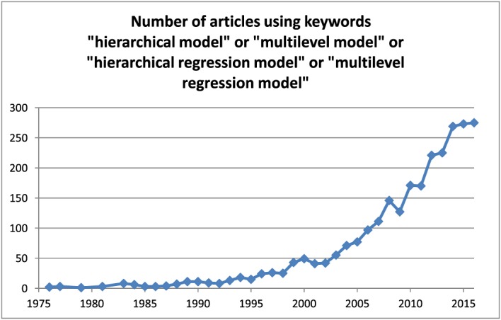
Number of articles using keywords ‘hierarchical model’ or ‘multilevel model’ or ‘hierarchical regression model’ or ‘multilevel regression model’. [Colour figure can be viewed at wileyonlinelibrary.com]

When data have a multilevel structure, subjects within the same cluster (e.g., hospital) may have responses or outcomes that are correlated with one another due to the exertion of a common, general contextual effect—the effect of the hospital environment itself (e.g., degree of specialization and skills of the staff, access to technology and efficient administrative processes, etc.) on the outcomes. Thus, two randomly selected patients from the same hospital may have outcomes that are more similar than the outcomes of two randomly selected subjects from different hospitals (even when the measured characteristics of the selected subjects are identical to one another). Multilevel regression models are a statistical technique that allows one to properly analyze multilevel data 1, 2, 3, 4. Such models incorporate cluster‐specific random parameters that account for the dependency of the data by partitioning the total individual variance into variation due to the clusters or ‘higher‐level units’ and the individual‐level variation that remains. The use of MLRM in epidemiology and health services research is relevant for both formal statistical and substantive epidemiological reasons 5.

From a statistical perspective, a condition for performing conventional regression analyses is that, conditional on the covariates (or predictor variables), the outcomes are independent across subjects. If the observed outcomes are not independent of one another, the effective sample size decreases, so that failure to account for the intra‐cluster correlation in conventional analyses falsely increases the precision of the estimates. Also, when formally comparing hospitals (or any other cluster) in a conventional regression analysis, we need to introduce dummy variables for the individual hospitals, which is an inefficient and non‐parsimonious strategy. Furthermore, it also prevents the study of the association between specific hospital characteristics and the individual outcome 6. In contrast to this, another advantage of MLRM is that it introduces only one random parameter for the entire population of hospitals and allows the simultaneous estimation of measures of association at different levels of the data hierarchy (e.g., hospitals and patients) 7. Furthermore, in conventional regression analysis, an individual level association (e.g., the association between a patient's age and mortality) is assumed to be of the same magnitude in all hospitals. However, in MLRM, we can relax this assumption and allow the magnitude of individual level associations to vary across clusters. In so doing, we can obtain a better understanding of the underlying heterogeneity in the data than is possible from a conventional regression analysis. Nevertheless, many researchers applying MLRM today still consider the intra‐cluster correlation as a kind of ‘nuisance’ that only needs to be accounted for in order to obtain correct estimations of uncertainty around regression coefficients and do not seem to be fully aware of the analytical and substantive advantages of MLRM 5, 8, 9, 10.

From a substantive epidemiological perspective, the purpose of MLRM is not restricted to simply accounting for the within‐cluster correlation in order to make correct estimates of measures of association. Rather, as expressed by Rodriguez and Goldman 11:

‘Estimates of the extent to which observations within a given group are correlated with one another are valuable not only for obtaining improved estimates of fixed effects and their standard errors but also for yielding important substantive information. In particular, estimates of the extent of similarity of observations within a cluster, with and without the introduction of a set of control variables, may provide insights into the influence of group level effects on individual behaviour and the pathways through which these effects operate’ (page 74).

This general contextual effect deserves attention on its own. Knowing the proportion of overall individual variation in a health outcome that is attributable to the contextual‐level (i.e., the intra‐cluster correlation) is of fundamental relevance for operationalizing contextual phenomena and for identifying the relevant levels of analysis 6, 7, 8, 12, 13, 14, 15, 16. The larger the share of the total outcome variance that is due to between‐cluster variation, the more relevant is the cluster‐level of analysis 6.

Besides the need for an explicit interpretation of the general contextual effect in MLRM, many authors and analysts may still be unaware of the correct interpretation of measures of association between cluster‐level covariates and individual‐level outcomes obtained by multilevel logistic regression models, which differs from the normal single‐level approach. Many of the early developers of multilevel models worked within the field of education research 2, 4. Consequently, the focus of much of their writing was on the hierarchical linear model, as outcomes are frequently continuous in education research (e.g., test scores). However, in biomedical research, outcomes are often binary in nature (e.g., success vs. failure of treatment; death vs. survival after an operation or procedure). With the hierarchical linear model, unlike with the multilevel logistic regression model, regression coefficients have the same interpretation as a conventional model in which clustering is not present.

Focusing on health care epidemiology, the objective of the current study is to provide a detailed tutorial illustrating concepts around the use of the multilevel logistic regression model, complementing previous publications of ours 10, 15. We illustrate key concepts through an empirical case study in which we use a series of multilevel logistic regression models to study variation in outcomes for patients hospitalized with an AMI. We restrict our study to a straightforward hierarchical two‐level structure with a random intercept. The paper is structured as follows: In Section 2, we introduce statistical models for the analysis of multilevel data with binary outcomes. In Section 3, we introduce the data that will be used for the subsequent case study analyzed in Section 4. In the case study, we conduct a series of analyses to illustrate issues around the application and interpretation of multilevel logistic regression models. Finally, in Section 5, we provide a short discussion and summarize our tutorial.

2. Statistical models for the analysis of multilevel data with binary outcomes

In this section, we introduce the basic random intercept logistic regression model that will be used throughout the remainder of this tutorial. The model derives its name from the fact that the intercept is allowed to vary randomly across clusters through the introduction of cluster‐specific random effects. In the formulas that follow, let Y_ij denote the binary response variable measured on the ith subject within the jth cluster (Y_ij = 1 denotes success or the occurrence of the event, while Y_ij = 0 denotes failure or lack of occurrence of the event). Furthermore, let X_1ij, through X_kij denote the k predictor or explanatory variables measured on this subject (e.g., patient age). Finally, let Z_1j, through Z_mj denote the m predictor variables measured on the jth cluster (e.g., hospital academic status).

The conventional multilevel logistic regression model incorporates cluster‐specific random effects to account for the within‐cluster correlation of subject outcomes:

$$\text{logit}\left(Pr\left(Y_{\mathit{ij}}=1\right)\right)={\alpha }_0+{\alpha }_{0j}+{\alpha }_1{x}_{1\mathit{ij}}+\cdots +{\alpha }_k{x}_{\mathit{kij}}+{\beta }_1{z}_{1j}+\cdots +{\beta }_m{z}_{\mathit{mj}}$$ (1)

where α_0j ~ N(0, τ²). The assumption is made that the random effects are independent of the model covariates (X,Z). In the case study below, we fit several variations of this model to the data and conduct a sequence of ancillary analyses that will enrich our interpretation of the data.

3. Data for case study

We used data from the Ontario Myocardial Infarction Database (OMID), which contains data on patients hospitalized with an AMI at Ontario hospitals between 1992 and 2014 17. For the case study, we used hospitalizations that occurred in the 12‐month period between April 1, 2013 and March 31, 2014. Due to the study inclusion and exclusion criteria, no patient had more than one hospitalization during the one year time frame of the study 17. The data have a multilevel structure, with patients nested within hospitals. The study sample consisted of 18 027 patients treated at 154 hospitals. The number of patients treated per hospital ranged from one to 962, with a median of 55 (25th–75th percentiles: 17–144).

Eleven patient‐level variables, consisting of the variables in the Ontario AMI Mortality Prediction model (age, sex, congestive heart failure, cardiogenic shock, arrhythmia, pulmonary edema, diabetes mellitus with complications, stroke, acute renal disease, chronic renal disease, and malignancy) were measured on each patient 18. The one continuous explanatory variable (age) was centered around the sample average (this was achieved by subtracting the average value of age in the entire cohort from each subject's age).

Three hospital‐level variables were included: hospital academic status (teaching hospital vs. non‐teaching hospital), hospital capacity for coronary revascularization (the presence of facilities for conducting coronary artery bypass graft surgery or percutaneous coronary intervention), and hospital volume of AMI patients (number of AMI patients treated during the year). The first two are binary, while the third is continuous. Hospital volume of AMI patients was centered around the overall cohort average (the cohort average of hospital AMI volume was computed as the weighted average of the individual hospital AMI volumes when hospitals were weighted by the number of patients at the given hospital).

The binary outcome for the case study was death due to any cause within one year of hospital admission, which occurred for 2805 (15.6%) patients in the sample.

Statistical software code for conducting the case study, in the R and SAS statistical programming languages, is provided in the Appendix.

4. Case study

4.1. Fitted multilevel logistic regression models

We fit three multilevel logistic regression models. The first was the null model which did not contain any patient or hospital characteristics. It incorporated only hospital‐specific random effects to model between‐hospital variation in mortality (Model 1). The second model included the 11 patient characteristics described above in addition to hospital‐specific random effects (Model 2). The third model included both patient characteristics and the three hospital characteristics described above in addition to hospital‐specific random effects (Model 3). Estimated regression coefficients and odds ratios are reported in Tables 1 and 2, respectively. The odds ratios were obtained by exponentiating the estimated regression coefficients. In Table 1, we also report the estimates of the variance of the distribution of the random effects.

Table 1.

Estimated regression coefficients and variance components for the multilevel logistic regression models.

Variable	Model 1	Model 2		Model 3
		Regression coefficient (95% CI)	P‐value	Regression coefficient (95% CI)	P‐value
Patient characteristics
Intercept	−1.565(−1.644,−1.486)	−2.635 (−2.734,−2.535)	<0.0001	−2.697 (−2.817,−2.578)	<0.0001
Age (per 10‐year increase)		0.752 (0.709,0.795)	<0.0001	0.746 (0.703,0.789)	<0.0001
Female		−0.009 (−0.105,0.086)	0.8476	−0.009 (−0.105,0.086)	0.8514
Congestive heart failure		0.728 (0.616,0.841)	<0.0001	0.727 (0.615,0.839)	<0.0001
Cerebrovascular disease		0.547 (0.195,0.898)	0.0023	0.521 (0.169,0.872)	0.0037
Pulmonary edema		0.483 (−0.178,1.143)	0.1520	0.470 (−0.189,1.13)	0.1622
Diabetes with complications		0.380 (0.282,0.478)	<0.0001	0.378 (0.280,0.476)	<0.0001
Malignancies		1.687 (1.475,1.898)	<0.0001	1.678 (1.467,1.890)	<0.0001
Chronic renal failure		0.539 (0.352,0.727)	<0.0001	0.534 (0.347,0.722)	<0.0001
Acute renal failure		0.821 (0.660,0.983)	<0.0001	0.823 (0.661,0.984)	<0.0001
Cardiogenic shock		2.284 (2.026,2.542)	<0.0001	2.314 (2.055,2.572)	<0.0001
Cardiac dysrhythmias		0.442 (0.323,0.560)	<0.0001	0.441 (0.322,0.559)	<0.0001
Hospital characteristics
Teaching hospital				−0.108 (−0.324,0.108)	0.3277
Hospital volume (per 100 increase in patients)				−0.052 (−0.087,−0.016)	0.0044
Capacity for cardiac revascularization				0.138 (−0.131,0.407)	0.3139
Variance of random effects
τ2	0.1089	0.0463		0.0332
PCV	Reference	57.5%		69.5%
VPC or ICC	0.032	0.014		0.010
MOR	1.37	1.23		1.19
PCV: proportional change of the variance, VPC: variance partition coefficient, ICC: intra class correlation, MOR: median odds ratio.

Table 2.

Estimated odds ratios for multilevel logistic regression models.

Variable	Odds ratio (95% CI)
	Model 2	Model 3
Patient characteristics
Age (per 10‐year increase)	2.12 (2.03,2.22)	2.11 (2.02,2.20)
Female	0.99 (0.90,1.09)	0.99 (0.90,1.09)
Congestive heart failure	2.07 (1.85,2.32)	2.07 (1.85,2.31)
Cerebrovascular disease	1.73 (1.22,2.45)	1.68 (1.18,2.39)
Pulmonary edema	1.62 (0.84,3.14)	1.60 (0.83,3.10)
Diabetes with complications	1.46 (1.33,1.61)	1.46 (1.32,1.61)
Malignancies	5.40 (4.37,6.68)	5.36 (4.33,6.62)
Chronic renal failure	1.72 (1.42,2.07)	1.71 (1.42,2.06)
Acute renal failure	2.27 (1.94,2.67)	2.28 (1.94,2.67)
Cardiogenic shock	9.82 (7.58,12.7)	10.11 (7.81,13.10)
Cardiac dysrhythmias	1.56 (1.38,1.75)	1.55 (1.38,1.75)
Hospital characteristics
Teaching hospital		0.90 (0.72,1.11)
POOR (%)		34
Hospital volume (per 100 increase in patients)		0.95 (0.92,0.98)
POOR (%)		42
Capacity for cardiac revascularization		1.15 (0.88,1.50)
POOR (%)		30

POOR: proportion of odds ratios in the opposite direction.

In the null model, the estimated intercept was −1.565, while the estimated variance of the random effects was 0.1089. Thus, at an average hospital (i.e., a hospital whose random effect was equal to zero on the logit scale), the probability of death within one year was $\frac{exp\left(-1.565\right)}{1+exp\left(-1.565\right)}=0.173$. The 95% probability interval for the hospital‐specific intercepts is (−2.212, −0.918) (i.e., 95% of hospitals will have a random intercept that lies within this interval). Thus, for 95% of hospitals, the hospital‐specific probability of death within one year would lie in the interval (0.099, 0.285). This was computed by taking the inverse logit transformation of the interval $-1.565\pm 1.96\times \sqrt{0.1089}$. Note that the predicted probability of death at an average hospital may differ from the average hospital‐specific probability of death because the integral of the hospital‐specific probability of death (i.e., $\frac{exp\left({\alpha }_0+{\alpha }_{0j}\right)}{1+exp\left({\alpha }_0+{\alpha }_{0j}\right)}$) over the distribution of the hospital‐specific random effects is not equal to $\frac{exp\left({\alpha }_0\right)}{1+exp\left({\alpha }_0\right)}$ (i.e., the previous quantity evaluated at the average random effect). Equivalently, the inequality holds because the average of the inverse logit function evaluated at a set of numbers is not equal to the inverse logit function evaluated at the average of the set of numbers.

In the model consisting of patient characteristics (Model 2), nine of the 11 patient characteristics were significantly associated with the odds of death within one year of hospital admission (Table 1). The two exceptions were female sex (odds ratio = 0.99, 95% CI = (0.90, 1.09)) and pulmonary edema (odds ratio = 1.62, 95% CI = (0.84, 3.14)). The intercept for this model was −2.635. Thus, at an average hospital (i.e., a hospital whose random effect was equal to zero), the probability of death within one year for a patient whose covariates were equal to zero was $\frac{exp\left(-2.635\right)}{1+exp\left(-2.635\right)}=0.067$. This reference patient is a male patient of average age and who did not have any of nine comorbid conditions or risk factors.

In the model that included both patient and hospital characteristics (Model 3), nine of the 11 patient characteristics were significantly associated with the log‐odds of death within one year, while only one of the three hospital characteristics (hospital volume of AMI patients) was significantly associated with the outcome (odds ratio = 0.95 per 100 patient increase in hospital volume, 95% CI = (0.92, 0.98)) (Table 1). Neither academic affiliation (odds ratio = 0.90, 95% CI = (0.72, 1.11)) nor capacity for cardiac revascularization (odds ratio = 1.15, 95% CI = (0.88, 1.50)) was significantly associated with one‐year mortality. The intercept for this model was −2.697. Thus, at an average hospital whose volume was equal to the average AMI volume, which did not have an academic affiliation and which did not have any capacities for cardiac revascularization, the probability of death within one year for a patient whose covariates were equal to zero was $\frac{exp\left(-2.697\right)}{1+exp\left(-2.697\right)}=0.063$. As above, this reference patient is a male patient of average age and who did not have any of nine comorbid conditions or risk factors.

4.2. Conditional or cluster‐specific interpretation of the multilevel logistic regression model

The odds ratios for the individual variables reported in Table 2 are conditional or cluster‐specific measures of association or intra‐cluster measures of association. This means that they are interpreted as having an effect conditional on the random effect being held constant [19]. Therefore, they may be interpreted as odds ratios for within‐cluster comparisons or, in our example, they are hospital‐adjusted associations between patient characteristics and mortality. In examining Model 2, one would interpret the odds ratio for age (2.12 per 10‐year increase in age) as suggesting that, when comparing two subjects whose age differs by 10 years, but who share identical values on the remaining 10 covariates and who also share the same hospital average risk (i.e., the value of the random effect), then the odds of death are 2.12 times higher for the patient who is 10 years older compared to the odds of death for the younger patient. In other words, when comparing two subjects within the same cluster who differ in age by 10 years, but who share identical values of the remaining ten covariates, the odds of death for the older subject is 2.12 times higher than the odds of death for the younger subject. It is important to note that the interpretation is conditional on both the other covariates as well as the cluster‐specific random effect (we can think of this odds ratio as having a similar interpretation to the one that we would obtain by adjusting for the hospitals as fixed effects using individual dummy variables for the individual hospitals—it is a measure of association after adjusting for both patient characteristics and the cluster). As these models implicitly control or condition on the cluster (i.e., the random effect), the covariate effects have a within‐cluster interpretation: what is the association between a specific patient characteristic (e.g., age) and the outcome, after controlling or adjusting for the remaining characteristics for subjects within the same cluster. We assume that the association between age and mortality is the same in all hospitals. That is, the hospital does not modify the effect of age on mortality.

The conditional interpretation of the regression coefficients does not present serious difficulties when considering a model that contains only subject characteristics (e.g., Model 2). However, it presents more serious difficulties when considering a model that incorporates cluster characteristics (e.g., Model 3). In Model 3, the odds ratio was 0.95 for an increase in hospital AMI volume by 100 patients. The conditional or within‐cluster interpretation of this coefficient is that, after fixing the patient characteristics and the other two hospital characteristics, and after fixing the random effect, an increase in hospital volume by 100 patients is associated with a 5% decrease in the odds of death. Thus, within a given hospital, an increase in hospital volume by 100 patients is associated with a 5% decrease in the odds of death. This interpretation is problematic as hospital volume is fixed within hospitals (i.e., when conditioning on random effects).

In other words, for a cluster‐level variable, the concept of an intra‐cluster association is not as straightforward as in the case of individual‐level variables because the value of the cluster level variable is constant for all individual in the cluster. Therefore, one needs to assume the existence of several clusters (i.e., hospitals) with the same characteristics, including a similar average risk (i.e., a similar residual or random effect) but with a different hospital volume. In this case, an increase in hospital volume by 100 patients is associated with a 5% decrease in the odds of death. This is an extreme extrapolation with an odd interpretation. However, most multilevel analyses published so far do not consider this limitation in interpretation. Neuhaus and McCulloch suggest that cluster‐specific models (such as those that incorporate cluster‐specific random effects) are best used to determine the association between within‐cluster changes in covariates and the outcome 20 (page 861). In order to address this limitation in how to interpret the effect of cluster‐level covariates, in the subsequent two sub‐sections, we introduce three alternative ways of presenting cluster level associations: the concept of marginal or population‐average regression coefficients, the interval odds ratio (IOR), and the proportion of opposed odds ratios (POOR). These quantities are necessary for an appropriate assessment of the magnitude of the association between outcomes and the characteristics of clusters.

4.3. Marginal or population‐average regression coefficients and odds ratios

As discussed above, multilevel logistic regression gives cluster‐specific measures of associations (ORs) that are, therefore, adjusted for ‘α_0j’ (the unobserved cluster effect). This is intuitive for individual‐level variables, but less clear for cluster‐level variables because there is no within‐cluster variation in the given cluster characteristic. An alternative method to the multilevel regression model for analyzing correlated data is the use of generalized estimation equations (GEE) with robust standard errors, which produces ‘population average’ odds ratios. The population‐average odds ratio is the average odds ratio comparing two subjects from two different clusters who are identical in other respects (apart from the covariate of interest) [19]. Because the estimated associations are not cluster specific, the interpretation of an association between a cluster level variable and the outcome is easier. In a review of cluster‐specific and population‐average models for clustered binary data, Neuhaus and colleagues demonstrated that under the cluster‐specific model, the estimated covariates from a population‐average model are closer to zero than are those from the cluster‐specific or conditional model 19. This is different from what occurs with the linear model, in which the cluster‐specific and population‐average effects coincide when outcomes are continuous 19.

Using multilevel analyses, it is possible to obtain an approximation of the population‐average coefficient based on the conditional or cluster‐specific regression coefficient using the following formula 21, 22:

$${\widehat{\alpha }}_{\mathrm{PA}}=\frac{{\widehat{\alpha }}_{\mathrm{CS}}}{\sqrt{1+\left({16}^2\times 3/{\left(15\times \pi \right)}^2\right)\times {\widehat{\tau }}^2}}$$ (2)

where ${\widehat{\alpha }}_{\mathit{CS}}$ is the estimated cluster‐specific or conditional regression coefficient (the log‐odds ratio) and ${\widehat{\tau }}^2$is the estimated variance of the distribution of the random effects. The denominator represents the shrinkage factor.

When using ${\widehat{\tau }}^2=0.0463$ and ${\widehat{\tau }}^2=0.0332$ for Models 2 and 3, respectively, the corresponding shrinkage factors are 1.008 (i.e., the population‐average log‐odds ratio is 0.992 × the conditional log‐odds ratio) and 1.006 (i.e., the population‐average log‐odds ratio is 0.994 × the conditional log‐odds ratio). As the two shrinkage factors are very close to one, the population‐average regression coefficients (and corresponding population‐average odds ratios) will be very close to the conditional or cluster‐specific regression coefficients (and corresponding odds ratios). When using Model 3, the population‐average odds ratios for the three hospital characteristics are essentially equal to the conditional or cluster‐specific odds ratios (to two decimal places).

4.4. Summary measures of the effects of cluster‐level variables

4.4.1. Interval odds ratio (IOR)

Larsen et al. proposed the IOR as a measure for quantifying the effect of cluster‐level variables when using multilevel logistic regression models 23, which was subsequently applied in epidemiology 21. Consider the distribution of the odds ratio comparing two subjects whose values of the given cluster‐level covariate differ by one unit (e.g., for a binary cluster‐level covariate, the condition is present in one cluster but absent in the other cluster), but who have identical values for the other cluster‐level covariates and of the subject‐level covariates. The IOR is an interval covering the middle 80% of the distribution of such odds ratios. The lower and upper bounds of this interval are given by

$$\begin{array}{l}\left.\begin{array}{l}{\mathrm{IOR}}_{\mathrm{L}}=exp(\alpha +\sqrt{2{\widehat{\tau }}^2}\times {\mathrm{\Phi }}^{-1}\left(0.10\right)\\ {\mathrm{IOR}}_{\mathrm{U}}=exp(\alpha +\sqrt{2{\widehat{\tau }}^2}\times {\mathrm{\Phi }}^{-1}\left(0.90\right)\end{array}\right\}\\ \end{array}$$ (3)

where α is the estimated regression coefficient associated with the given cluster‐level covariate, ${\widehat{\tau }}^2$ is the estimated variance of the distribution of the random effects, while Φ⁻¹(0.10) =  − 1.2816 and Φ⁻¹(0.90) = 1.2816 denote the 10th and 90th percentiles of a standard normal distribution.

The 80% IORs for the three hospital‐level characteristics in Model 3 were (0.65, 1.25) for academic hospitals vs. non‐academic hospitals, (0.68, 1.32) for an increase in hospital volume by 100 patients, and (0.83, 1.60) for the presence of revascularization facilities vs. the absence of such facilities.

As every exposure category of the cluster‐level variable contains many clusters, when the residual cluster variance is large, then the distributions of the clusters around the average outcome in the different exposure categories overlap each other. Therefore, when performing pairwise comparisons between exposed and unexposed clusters, the odds ratios will vary widely around the average odds ratio (i.e., a large 80% IOR). However, when the residual cluster variance is small, then the variability of the odds ratios will also be small (i.e., a small 80% IOR). Larsen and Merlo suggest that if the IOR contains one, then the cluster variability is large in comparison with the effect of the cluster‐level variable. If the IOR does not contain unity, then the effect of the cluster‐level variable is large in comparison with the unexplained between‐cluster variation 21. Thus, when comparing patients with identical characteristics, one selected from a hospital with an academic affiliation and one from a hospital with no academic affiliation, the odds of death will lie between (0.65 and 1.25) in 80% of such comparisons. As all three intervals contain one, we would conclude that even if the cluster variability is small as expressed by the median odds ratio (MOR) and the intraclass correlation coefficient (ICC) (see later section), this variability is large in comparison with the effect each of the three hospital‐level variables.

4.4.2. Proportion of opposed odds ratios

Merlo proposed the ‘sorting out index’ 15 or, using a more informative term, the POOR 10 as an alternative to the IOR as a measure of the magnitude of the effect of cluster variables. While the IOR describes the middle 80% of the distribution of odds ratios comparing a random cluster exposed to the covariate and a random cluster not exposed to the covariate, the POOR is the proportion of such odds ratios with the opposite direction to the overall odds ratio. The POOR is evaluated as

$$\text{POOR}=\mathrm{\Phi }\left(-\left|\frac{\alpha }{\sqrt{2{\widehat{\tau }}^2}}\right|\right)$$ (4)

where α denotes the regression coefficient associated with the given cluster characteristic, and ${\widehat{\tau }}^2$ denotes the variance of the distribution of the random effects.

The POOR can take values ranging from 0 to 50%. A POOR of 0% implies that all pair‐wise odds ratios are in the same direction as the overall cluster‐specific odds ratio. A POOR of 50% means that half of the pair‐wise comparisons between clusters exposed to the condition and clusters non‐exposed to the condition are in the direction opposite to the overall odds ratio. A larger value for the POOR implies that the association is very heterogeneous.

In our case study data, the POOR for hospital teaching status was 0.34, the POOR for a 100 increase in hospital volume of AMI patients was 0.42, while it was 0.30 for hospital revascularization status. Thus, in 34% of comparison between a teaching hospital and a non‐teaching hospital, the odds ratio for this comparison would be different in direction to that of the overall odds ratio for teaching status. The overall odds ratio was 0.90 (Table 2), denoting decreased mortality at teaching hospitals. However, in 34% of pair‐wise comparisons, the odds of death would be higher at the teaching hospital than at the non‐teaching hospital. To interpret the POOR, we need a systematic approach that begins with the evaluation of the general contextual effect in a model adjusted for individual‐level variables (i.e., Model 2). We then seek to understand the specific contextual mechanisms behind the general contextual effect. To do so we include hospital‐level variables (i.e., Model 3). If the hospital‐level variables are relevant, then they would be associated with the outcome and they would also explain some of the variance of the random intercepts from Model 2. In this scenario, the variance of the random effects from Model 3 would be smaller than the variance of the random effects from Model 2, and the POOR would tend to zero. In our case study, the Model 2 general contextual effects were initially small (as indicated by the ${\widehat{\tau }}^2$and the VPC), and the hospital‐level variables explained about 28% of the variance of the random effects from Model 2. However, the random effects variance from Model 3 was large enough to produce rather heterogeneous associations for the hospital‐level variables. As explained previously, complete heterogeneity would correspond with a POOR of 50%. In our study, the heterogeneity was appreciable as the POORs were higher than 30% for all three hospital‐level variables (see elsewhere for further explained examples on the interpretation of the POOR) 10.

4.5. Measures of components of variance and of heterogeneity

The analyses reported in the previous sub‐sections permit the analyst to estimate measures of association. That is, the association between the odds of the occurrence of the outcome and subject‐ and cluster‐level covariates. However, the estimated coefficients and odds ratios do not provide a measure of general contextual effects, which are fundamentally based on an analysis of variance 14, 24.

To estimate general contextual effects (that is, the effect of the cluster itself on subject outcomes), we need measures of components of variance (e.g., clustering) and of heterogeneity. In this section, we describe the variance partition coefficient (VPC) or the more specific ICC for hierarchical structures. We also describe the MOR for quantifying variation or heterogeneity in outcomes between clusters.

4.5.1. The variance partition coefficient

The VPC represents the proportion of the total observed individual variation in the outcome that is attributable to between‐cluster variation. The higher this proportion, the higher is the general contextual effect. Given a continuous outcome, and if σ²and τ²denote the between‐subject and between‐cluster variation (e.g., obtained from a variance components model), then we have that $\mathrm{VPC}=\frac{{\tau }^2}{{\tau }^2+{\sigma }^2}$. For simple hierarchical structures like patients nested within hospitals, the VPC is equivalent to the ICC. Besides being a VPC, the ICC can be interpreted as the correlation in the outcome between two individuals randomly selected from the same cluster. In a multilevel linear model, both the between‐subject and the between‐cluster variance can be derived directly from the fitted model and the VPC is intuitively easy to understand.

Nevertheless, the VPC or the ICC is less easy to understand and calculate when analyzing binary responses following a binomial distribution in a multilevel model. One can estimate directly the between‐cluster variation—it is the variation of the distribution of the cluster‐specific random effects. However, in a multilevel regression model for binary outcomes, unlike in a conventional multilevel linear regression model, there is no direct estimate of σ², the between‐subject variance. For a binary response, the variance of a binomial distribution is completed determined by the mean (as the binomial variance is a function of the mean of the binomial distribution). Furthermore, the between‐cluster variance is defined on a different scale (e.g., the log‐odds scale in a logistic regression), than the binary response scale 5.

Nevertheless, there are a variety of procedures for calculating the VPC for binary responses, including a normal response approximation, the simulation method, the Taylor series linearization, and the latent response formulation 5, 15, 25, 26. Basically, these procedures convert both the between‐cluster and the within‐cluster component of the individual variance to the same scale, which allows one to compute a VPC 27. Note that these methods for calculating the VPC differ from methods for estimating the ICC in a cluster‐randomized trial with a binary outcome 28.

Among these different procedures, the VPC based on the latent response formulation of the model has become the most widely used. Under this procedure, it is assumed that the binary outcome variable arises as the dichotomization of an underlying continuous latent variable following a logistic or a probit distribution. That is, the regression uses a logit or a probit link function, respectively. The variance of a logistic distribution with scale parameter equal to one is $\frac{{\pi }^2}{3}$ 29. The between‐subject variance is equal to one in the probit case that follows a standard normal distribution 1, 5, 30. Thus, one can evaluate the VPC as $\frac{{\widehat{\tau }}^2}{{\widehat{\tau }}^2+\frac{{\pi }^2}{3}}$ when using a logit link or $\frac{{\widehat{\tau }}^2}{{\widehat{\tau }}^2+1}$when using the probit link. Empirically, it is easy to prove this assumption by calculating the ICC for a continuous outcome and then calculating the ICC for dichotomizations of the continuous outcome. The results tend to be similar between the two approaches. However, when the prevalence of the dichotomization is extreme (i.e., very low or very high), then the probit link is more appropriate than the logit link.

In our data, the estimate of the between‐hospital variance was 0.1089 for Model 1, 0.0463 for Model 2, and 0.0332 for Model 3. These correspond to VPCs of 0.032, 0.014, and 0.010, respectively. The first of these has an unconditional interpretation, while the latter two have a conditional or residual interpretation. The VPC derived from the null model was 0.032. This implies that 3.2% of the individual variation in the underlying propensity to die within one‐year is due to systematic differences between hospitals (without considering the possibility of a different patient‐mix composition when estimating the hospital variance), while the remaining 96.8% is due to systematic differences between patients.

The second and third VPCs have a conditional interpretation: of the residual variation in outcomes that remains after accounting for the variables in the model, it is the proportion that is attributable to systematic differences between clusters. Thus, when using Model 2, we would infer that of the residual variation in outcomes that persists after adjusting for 11 patient characteristics, 1.4% is due to systematic differences between hospitals, while the remaining 98.6% is due to unmeasured differences between patients.

Goldstein et al. 5 suggest that the approach to evaluating the VPC or the ICC described above is appropriate when the binary response can be conceptualized as the discretization of an underlying continuous latent variable (e.g., pass/fail on a test is a binary representation of an underlying continuous latent variable denoting the test score). For a binary outcome such as mortality, they suggest that such an assumption may not be warranted as it is unobservable. On the other hand, one can assume that there is an underlying propensity of dying and that an individual dies when he/she reaches a certain threshold. Goldstein et al. described a simulation‐based approach that does not require this assumption. However, a characteristic of this simulation‐based approach is that it is dependent on specific covariate patterns. Thus, one could conceivably have a different value of the VPC for each distinct covariate pattern (this could be of substantive interest in and of itself). Their proposed algorithm is as follows:

1. Simulate a large number of cluster‐level random effects from the random effects distribution that was obtained from fitting the multilevel logistic regression model: ${\mu }_i˜N\left(0,{\widehat{\tau }}^2\right)$, for i = 1 ,  …  , M.

2. For a specific covariate pattern, use each of the simulated random effects drawn in Step 1 to compute the predicted probability,p_i, of the outcome using the fitted multilevel logistic regression model. For each of these computed probabilities, compute the Level 1 variance: v_i = p_i(1 − p_i).

3. The VPC is then evaluated as $\frac{\mathrm{Var}\left(p_i\right)}{\mathrm{Var}\left(p_i\right)+\frac{1}{M}\sum _{i=1}^M{v}_i}$.

We used the above algorithm with 50 000 iterations. Using the data from our case study, the VPC for the null model was 0.016. For a reference patient whose covariates were equal to zero (i.e., a male of average age with no comorbidities or risk factors), the VPC for Model 2 was 0.003. For a reference patient whose covariates were equal to zero (i.e., a male of average age with no comorbidities or risk factors and who was treated at a non‐academic hospital with average volume and no facilities for cardiac revascularization), the VPC for Model 3 was 0.002. While these estimates of the VPC differ from those obtained above, the interpretation would remain the same: the general contextual effect was small. That is, there was relatively little systematic between‐hospital variation in outcomes, with the large proportion of variation being attributable to between‐subject variation.

In practice, it appears that the method based on the latent variable approach is used more frequently than the simulation approach described by Goldstein et al.

The VPC (or the ICC) is a key concept in multilevel analysis as it quantifies the proportion of observed variation in the outcome that is attributable to the effect of clustering. The VPC would be equal to one if all subjects in the same cluster exhibited the same response. However, the VPC would be equal to zero if the there was no within‐cluster homogeneity of responses. We refer readers to further discussion of this statistic in the multilevel literature 1, 2, 30, 31, 32, 33.

4.5.2. Median odds ratio

The MOR was first proposed by Larsen et al. 23 for quantifying the magnitude of the effect of clustering when using a multilevel logistic regression model. It was subsequently popularized in the epidemiological literature by Larsen and Merlo 21. If one were to repeatedly sample at random two subjects with the same covariates from different clusters, then the MOR is the median odds ratio between the subject at higher risk of the outcome and the subject at the lower risk of the outcome (differences in risk are entirely quantified by the cluster‐specific random effects). The MOR can be evaluated as:

$$\mathrm{MOR}=exp\left(\sqrt{2{\widehat{\tau }}^2}\times {\mathrm{\Phi }}^{-1}\left(0.75\right)\right)$$ (5)

where ${\widehat{\tau }}^2$is the estimated variance of the distribution of the random effects, Φ denotes the cumulative distribution function of the standard normal distribution, while Φ⁻¹(0.75) = 0.6745 is the 75th percentile of a standard normal distribution.

In our data, the MOR was equal to 1.37 (Model 1), 1.23 (Model 2), and 1.19 (Model 3). In interpreting the MOR from Model 2, we would say that when comparing two identical patients from randomly selected hospitals, the MOR comparing a patient at the hospital with the higher risk of death to a different patient (but with the same covariate values) at the hospital with the lower risk of death was 1.23. Thus, in half such comparisons, the odds of death would be less than 1.23 for a patient at the hospital at higher risk compared to a different patient (but with the same covariate values) at the hospital at lower risk.

An advantage to use of the MOR for quantifying the contextual effect is that it is on the same scale as that used for estimating measures of association when quantifying the effect of subject‐level (and cluster‐level) covariates on the odds of the outcome. Thus, one can compare the magnitude of the MOR with that of the association between characteristics of the subject and the outcome. When considering Model 2, the MOR was 1.23. The reciprocal of this quantity is 0.81. In examining the odds ratios for Model 2 (Table 2), we observed that 10 of the 11 patient characteristics had an odds ratio that lay outside of the interval (0.81, 1.23). Thus, the magnitude of the effect of clustering (the contextual effect) was smaller than that of 10 of the 11 patient characteristics.

Even if both the ICC and the MOR are functions of the same between‐cluster variance, ${\widehat{\tau }}^2$, the MOR is a measure of heterogeneity while the VPC (ICC) is a measure of components of variance (clustering) that considers both between‐ and within‐cluster variance. Therefore, technical difficulties apart, the VPC provides improved estimation of the general contextual effects (or the contextual phenomenon) 6. If the VPC (ICC) was close to 0, then outcomes for patients from the same hospital would be no more similar that outcomes for a random sample of patients from the population. On the other hand, if the VPC (ICC) was close to 1, then all patients in the same hospital would have exactly the same outcome. In this way, multilevel analysis helps answer a traditional question among epidemiologist in health services research: ‘What is too much variation?’ 34. From a multilevel analytical perspective, this traditional question is easily answered by the VPC (ICC). That is, rather than only quantifying if the hospital variance is statistically significantly different from zero, hospital variation can be considered large only when the hospital variance corresponds to a large share of the total individual variance. The VPC (ICC) considers both the within‐ and between‐hospital variation, and its value ranges from zero to one. The MOR, however, considers only the hospital variance, and its value can range from one to infinity, which makes its magnitude more difficult to interpret. We suggest that when interpreting the magnitude of the MOR, it is convenient to relate its value to the size of the VPC (ICC). Therefore, in the present empirical analysis, we would interpret the MOR of 1.23 as low because it corresponds to a VPV (ICC) of 0.014. That is, only 1.4% of the total variation in patient mortality is due to between‐hospital differences in mortality.

The ICC could also be considered as a kind of measure of discriminatory accuracy that, similarly to the area under the curve (AUC) for use with logistic regression models, informs on the relevance of the clusters for identifying individual with and without the outcome 35, 36.

4.6. Proportional change in cluster variation

In this section, we describe the proportional change in cluster variance which is frequently used to quantify the variation explained by a multilevel model 12. Let ${\widehat{\tau }}_{\text{full}}^2$and ${\widehat{\tau }}_{\text{null}}^2$denote the estimated variances of the distribution of the random effects for the full model and the null model, respectively. Then, the proportional reduction in between‐cluster variance is defined by:

$$\frac{{\widehat{\tau }}_{\text{null}}^2-{\widehat{\tau }}_{\text{full}}^2}{{\widehat{\tau }}_{\text{null}}^2}$$ (6)

In our case study data, the proportional change in cluster variance comparing the null model (Model 1) with the model with patient characteristics (Model 2) was 0.575. The proportional change in cluster variance comparing the null model with the full model containing both patient and hospital characteristics (Model 3) was 0.695.

The proportional change in cluster variance is relatively unproblematic and easy to interpret in hierarchical linear models for continuous outcomes. In the case of a continuous outcome, the addition of a subject‐level covariate may explain some of the individual‐level variation (thereby decreasing the individual‐level variance compared to that of the simpler model without the given covariate). Consequently, the cluster‐level variance increases in magnitude relative to the individual‐level variance, with the result that the VPC (ICC) increases. However, this is not the case for binary outcomes. When outcomes are binary, the subject‐level variance is fixed when using the latent variable formulation (being π²/3 when using the logit link and 1 when using the probit link). Thus, each time that a variable is added to the model, the underlying latent variable is rescaled so that its between‐subject variance remains unchanged (at either π²/3 or 1). Thus, the between‐subject variation cannot decrease as a result of the addition of subject‐level covariates. A consequence of this rescaling of the underlying latent variable is that the cluster‐level variation is also rescaled 30. The result of these underlying rescalings is that the variance components cannot be compared directly between models. A resultant increase in the between‐cluster variance may be interpreted as the clusters appearing to become more ‘relevant’ after adjusting for their individual composition. For instance, in epidemiology an increase in cluster‐level (e.g., neighborhood), variance is often observed after adjusting for individual age in multilevel analyses of mortality, thus appearing to reveal a higher general contextual effect. Therefore, an increased proportional change in cluster variance in a multilevel logistic regression after inclusion of individual‐level variables needs to be interpreted with caution. In contrast to the proportional change in cluster variance, the VPC (ICC) is a meaningful measure because it is a ratio between the cluster and the total individual variance. Also, note that the rescaling issue only occurs when the between‐subject variation is explained. If our interest is to quantify the reduction in the cluster variance after adjusting for individual‐level variables in absolute terms, we need to rescale the variance to that of the initial model 27. This rescaling issue affects all generalized linear models and is not specific to multilevel logistic regression. In the null model, the total variance is ${\sigma }_0^2={\tau }^2+{\pi }^2/3$ (when using the logistic latent variable approach), where τ² denotes the variance of the random effects. In a model with subject characteristics, the total variance is ${\sigma }_1^2={\tau }^2+{\pi }^2/3+{\sigma }_F^2$, where τ² denotes the variance of the random effects and ${\sigma }_F^2$ denotes the variance of the linear predictor from the fixed part of the model. Then, the scale correction factor for the variance terms is ${\sigma }_0^2/{\sigma }_1^2$. A short but informative discussion is given by Hox 30 (pages 133–138).

When comparing the model with patient characteristics (Model 2) with the null model (Model 1), the scale correction factor for the variance terms was equal to 0.64. When this correction factor was applied to the variance of the random effects, the resultant proportional reduction in variance was 0.737. This indicates that the reduction in between‐cluster variation was greater after the rescaling had been taken into account than when it was ignored.

It bears stressing that a consequence of this rescaling is that the proportional change in cluster variance when outcomes are binary does not behave like an R ²‐type statistic. Both Kyle et al. and Snijders and Bosker describe how, in multilevel models for binary data, the inclusion of additional covariates can result in an increase in the variance of the distribution of the random effects 1, 37. This is unlike the conventional R ² statistic for a linear regression model, in which the addition of covariates will never result in a reduction in the model R ². Thus, while this measure has some utility, it should not be treated like a measure of R ², as it does not have some of the desirable properties of an R ² statistic. This is a direct consequence of the rescaling of the underlying latent variable so that it has a constant between‐subject variance.

4.7. Measuring the magnitude of the contextual effect using change in the model c‐statistic

Merlo et al. proposed that the magnitude of the general contextual effect could be assessed by a stepwise examination of discriminatory accuracy 10. The c‐statistic, which is equivalent to the area under the receiver operating characteristic (ROC) curve, is a commonly used measure for summarizing the discriminatory ability of a binary prediction model. When comparing all possible pairs of subject comprised of one subject who experienced the event of interest (e.g., mortality) and one subject who did not experience the event of interest, the c‐statistic is the proportion of such pairs in which the subject who experienced the event had a higher predicted probability of experiencing the event than did the subject who did not experience the event 38.

The ROC curve is constructed by plotting the true positive rate (TPR) (i.e., sensitivity) against the false positive rate (FPR) (i.e., 1 − specificity) for different binary classification thresholds of the predicted probabilities. The AUC measures the ability of the model to correctly classify individuals with or without the outcome as a function of individuals' predicted probabilities. The AUC takes a value between 0.5 and 1, where 1 denotes perfect discrimination and 0.5 would be as equally as informative as flipping a coin (i.e., the covariates have no predictive power). Merlo et al. proposed that one could quantify the general contextual effect by measuring the change of the ROC curve after adding a random effect for the cluster‐level to a singel‐level model that only contains individual level variables without any cluster‐level random effect 10.

We fit a sequence of three logistic regression models for predicting 1‐year mortality. The first regression model contained only the 11 patient characteristics described previously. It contained only fixed effects and did not contain any hospital‐specific random effects. The second model contained the 11 patient characteristics described previously and hospital‐specific random intercepts (Model 2). The third model added the three hospital characteristics to the second model (Model 3). The c‐statistics of these three models were 0.832, 0.836, and 0.836, respectively. Thus, accounting for the context of care (through the inclusion of hospital‐specific random effects) resulted in an increase in the c‐statistic of 0.004. However, the inclusion of hospital characteristics had no further effect on model discrimination (strictly speaking, the addition of hospital characteristics resulted in a negligible decrease in the discriminatory accuracy; however, this was only evident in the fourth decimal place). As discussed elsewhere 10, 39, the addition of cluster (e.g., hospital) characteristics to the model that contains cluster‐specific random effects cannot increase the c‐statistic of the model containing only the cluster‐specific random effects. Thus, the increase in the c‐statistic that arises from the inclusion of random effects in the model that contained only patient characteristics represents the ceiling of the hospital's general contextual effect.

In our empirical example, we found only evidence of a weak general contextual effect, as the inclusion of hospital random effects resulted in only a negligible increase in the discriminatory accuracy.

4.8. Proportion of variation explained by the multilevel logistic regression model

When fitting multilevel models, the analyst is frequently interested in quantifying the proportion of observed variation that is explained by the fitted model. A large number of R ²‐type measures have been proposed for use with multilevel linear regression models 1, 37. However, a limitation of these measures is that they are restricted to the multilevel linear model for use with continuous outcomes. Unfortunately, their definition does not carry over to the multilevel logistic regression model. In the context of binary outcomes, a wide number of measures of explained variation have been proposed for use with the conventional logistic regression model 40, 41. However, none of these methods incorporate cluster‐specific random effects.

Snijders and Bosker proposed a measure of explained variance for use with multilevel logistic regression models 1. As with the ICC, this method assumes that the binary outcome variable is generated through the dichotomization of an underlying latent continuous variable. Let τ² be the variance of the random intercept from the fitted multilevel logistic regression model. Furthermore, as with the intraclass correlation coefficient, assume that the level‐one residual variance is fixed at π²/3. For each subject in the sample, one determines the linear predictor based on the fixed effects. This is the predicted log‐odds of the outcome based on the model fixed effects. This can be evaluated using formula (1) with the cluster‐specific random effect (α_0j) removed from the linear predictor. Let ${\sigma }_F^2$ denote the sample variance of the fixed effects linear predictor. Then, the measure of proportion of variation explained can be computed as

$$R_{\text{binary}}^2=\frac{{\sigma }_F^2}{{\sigma }_F^2+{\tau }^2+{\pi }^2/3}$$ (7)

Using the case study data, the value of $R_{\text{binary}}^2$was 0.374 and 0.376 for Models 2 and 3, respectively. Thus, 11 patient characteristics and hospital‐specific random effects explained approximately 37% of the observed variation in one‐year mortality. The addition of hospital characteristics had essentially no effect on the proportion of variation explained. The null model explains 0% of the variation in mortality as there is no variation in the fixed intercept across hospitals ( ${\sigma }_F^2=0$).

Snijders and Bosker caution that proportions of variation explained for single‐level logistic regression models tend to be lower than corresponding statistics for ordinary least squares regression models.

4.9. Separating between‐ and within‐cluster covariate effects using partitioning methods

In formulating the random effects logistic regression model above (formula (1)), the assumption was made that the random effects are independent of the model covariates (X,Z). Ignoring such a correlation can lead to inconsistent estimation of the regression parameters 20. In settings in which a subject‐level covariate is correlated with the random effects, Neuhaus and colleagues suggest that a solution to inconsistent estimation of regression parameters is to partition the given covariate effect into between‐ and within‐cluster covariate effects 20, 42. The between‐cluster covariate is the cluster‐mean of the given covariate, while the within‐cluster covariate is the deviation of the covariate from the cluster‐mean of the covariate. Thus, if X_ij denotes the variable measured on the ith subject in the jth cluster, we partition this variable into a cluster‐level variable ${\overline{X}}_j$, denoting the mean of the variable in the jth cluster and a within‐cluster variable $X_{\mathit{ij}}-{\overline{X}}_j$, denoting the deviation from the cluster‐specific mean. Including terms for these two derived covariates in the regression model (and omitting the original covariate) can eliminate the bias due to correlation between the random effect and the covariate.

In our case study, we thought it unlikely that any of the subject‐level covariates were correlated with the random effects. However, to illustrate the application of the method and how the resultant model is interpreted, we partitioned age into between‐ and within‐cluster components. We modified Model 2 by removing the covariate for subject age and replacing it by the within‐ and between‐hospital components. The odds ratio for the within‐hospital component was 1.08 per year increase in age (95% CI: 1.07–1.08), while the odds ratio for the between‐hospital component was 1.11 (95% CI: 1.09–1.13).

The interpretation of the first odds ratio has a straightforward within‐cluster interpretation, as described above: within hospitals, a one‐year increase in age is associated with an 8% increase in the odds of death. However, as noted above and as described by Neuhaus and Kalbfleish, the second odds ratio is more difficult to interpret as it has a within‐cluster or conditional interpretation, but does not vary within hospitals 42. Using the estimate of the variance of the random effects (0.03600), one can compute the shrinkage factor as described above. The shrinkage factor is 1.006, so the corresponding population‐average regression coefficient is approximately equal to the conditional regression coefficient multiplied by 0.994. Thus, the population‐average odds ratio for the between‐hospital component of age was approximately equal to 1.11 (95% CI: 1.09–1.13). Thus, when comparing mortality between two identical patients treated at hospitals for which the average age of their patients differs by one year, the odds of death will be 11% higher for the patient treated at the hospital whose patients are, on average, one year older. This suggests that both increasing patient age, as well as an increase in the average age of patients treated at a hospital, are associated with patient mortality.

5. Discussion

Multilevel data occur frequently in a wide range of research fields. Researchers and analysts are increasingly aware of the need to account for the clustering of subjects within higher‐level units when fitting regression models to such data. However, frequently, analysts restrict their attention to the estimation of regression coefficients and the interpretation of fixed effects. Such restricted analyses do not take advantage of the opportunity provided by multilevel data to formally examine the magnitude of the effect of clustering. The limited scope of many applied analyses indicates the need for increased translational work introducing the potential depth and scope of multilevel analyses to applied analysts and researchers.

Multilevel logistic regression models result in odds ratios that have a cluster‐specific or within‐cluster interpretation. This can be particularly problematic for cluster‐level variables. In health services and social epidemiology research, such variables are often of great interest (e.g., hospital or neighborhood characteristics). We described methods to estimate the marginal or population‐average effect of cluster characteristics. These allow for the formal comparison of outcomes between different clusters whose characteristics differ from one another. We also described the IOR and the POOR that are summary measures of the effects of cluster‐level variables. These measures permit analysts to quantify the heterogeneity in the effect of cluster‐level variables.

As noted above, Rodriguez and Goldman suggest that between‐cluster variation is not simply a nuisance that must be accounted for in order to obtain accurate estimates of confidence intervals for fixed effects 11. Instead, study of between‐cluster variation in outcomes can be of substantive interest in itself. The VPC and the MOR permit the analyst to formally quantify the magnitude of the general contextual effect, by quantifying the magnitude of the variation in outcomes between clusters.

Finally, we described an R ² measure that is appropriate for use with multilevel logistic regression models. This measure permits analysts to quantify the proportion of variation in the response variable that is explained by the regression model. By comparing different models, one can formally quantify the proportion of variation that is explained by the addition of cluster‐level covariates.

A central assumption behind the models discussed in this tutorial is that the cluster‐specific random effects follow a normal distribution. This assumption underlies the model‐fitting algorithms of most of the commonly‐used statistical software packages for fitting multilevel logistic regression models. An important question is the effect of misspecification of the distribution of the random effects on estimation of the different components of a multilevel logistic regression model. In a study of the mixed‐effects logistic regression model, Neuhaus and colleagues demonstrated that when the random effects distribution is misspecified, then estimates of model parameters are asymptotically biased 43. However, they presented approximations that suggest that the bias in the estimated covariates effects is small in many settings. They concluded that ‘the mixed‐effects model yields inferences about the regression parameters that are quite robust to misspecification of the mixing distribution. In addition, valid standard error estimates of the estimated regression coefficients can be obtained using standard methods applied to the misspecified likelihood’ (page 761). Similarly, Heagerty and Kurland found that the asymptotic relative bias in estimated regression coefficients was small in nearly all of the scenarios that they examined 44 (see Table 1 of their paper). Furthermore, they found that the model‐based standard errors are approximately correct under model misspecification. Chen and colleagues similarly claimed that estimation of regression coefficients is subject to minimal bias when the distribution of the random effects is misspecified 45 (page 359). Finally, in a review on this topic, McCulloch and Neuhaus state that ‘virtually every study of the impacts of misspecification has shown little impact on within‐cluster covariates’ 46 (page 392). In the cause of cluster‐level covariates, they conclude that ‘bias in estimates of between‐cluster covariates has not been demonstrated. Efficiency loss has been demonstrated, but only in distributions quite far from non‐normality, indicating a high degree of robustness’ (page 393). Many of the measures of contextual effects that we have described are based on the estimate of the variance of the random intercepts. Thus, it is important to understand the magnitude of bias in estimation of this variance when the distribution of the random effects is misspecified. Across a range of scenarios, Heagerty and Kurland found that the asymptotic relative bias in estimating the standard error of the random effects distribution was at most 17% 44. In terms of estimating the variance of the random effects distribution, McCulloch and Neuhaus suggest that ‘estimation of the random effects variance appears relatively robust to misspecification of the random intercept distributional shape’ 46 (page 395).

A second assumption made above was that the subject and cluster covariates were independent of the random effects. In the last section of the case study, we have described how partitioning a subject‐level covariate into between‐ and within‐cluster components permits consistent estimation of regression parameters when the original subject‐level covariate was correlated with the random effects. However, in many settings, it may be the cluster‐level covariates that are correlated with the random effects. In health services research, there is a large literature on the effect of the number of surgical procedures carried out at a given hospital or by a given surgeon on patient outcomes 47. A consistent finding across a range of surgical procedures is that increasing hospital volume is associated with improved patient outcomes 48. In the context of multilevel analysis, this implies that if hospital (or surgical volume) is a variable in the model, then it may be negatively correlated with the random effects (hospitals with higher procedural volume will have lower mortality, and hence a smaller random effect). Neuhaus and McCulloch use the term ‘informative cluster size’ to refer to the setting in which the size of clusters (e.g., number of patients at a hospital) is related to components of the outcome regression model 49. When considering a generalized linear model with random intercepts, they found that ignoring informative cluster size results in consistent estimators of covariate effects when the true covariate effects are zero. Future research is required into improved methods of estimation if the true covariate effect differs from zero.

The focus of the current tutorial has been on the multilevel logistic regression model for the analysis of binary outcomes. For those interested in time‐to‐event or survival outcomes, we refer the reader to a recent tutorial on methods for the analysis of multilevel survival data and an article on the median hazard ratio, which is a measure of the general contextual effect when outcomes are time‐to‐event in nature 50, 51.

Incorporating the analyses described in the current article permit the analyst to gain a deeper understanding of the effect that the cluster (the general contextual effect) exerts on subjects, and the between‐cluster heterogeneity in outcomes.

Appendix A. SAS and R code for the case study analyses

A.1.

The SAS procedure GLIMMIX was used for fitting the multilevel logistic regression models in our case study. The subsequent analyses were conducted in R. We provide R code for fitting the multilevel logistic regression models. All of the analyses could have been conducted exclusively in SAS or exclusively in R.

/* Variables:

dth_1yr: binary variable denoting death within one year of admission.

age: age in years.

female: female sex.

chf: congestive heart failure.

cvd: stroke (cerebrovascular disease).

pulmoned: pulmonary edema.

diabcomp: diabetes with complications.

malig: malignancy.

crf: chronic renal failure.

arf: acute renal failure.

shock: cardiogenic shock.

carddys: cardiac arrhythmia.

teaching: teaching hospital.

hospvol: hospital volume of AMI patients.

hosp_revasc: hospital with cardiac revascularization capacity.

inst: hospital identifier.

ID: patient identifier.

*/

 

data cohort;

set cohort;

age = age/10;

hospvol = hospvol/100;

/* Age is in units of decades */.

/* Hospital volume is in units of 100 patients */.

run;

 

proc sort data=cohort;

by ID;

run;

 

proc logistic data=cohort descending;

model dth_1yr = age female chf cvd pulmoned diabcomp malig crf arf.

shock carddys;

output out=out1 (keep = ID dth_1yr pred1) pred=pred1;

title "Conventional logistic regression model that ignores clustering" ;

/* This model is used only for the ROC discrimination analysis */.

run;

 

proc glimmix data=cohort method=quad;

class inst;

model dth_1yr = /dist=binomial solution cl;

random intercept /subject=inst;

title “Null Multilevel logistic regression model”;

run;

 

proc glimmix data=cohort method=quad;

class inst;

model dth_1yr = age female chf cvd pulmoned diabcomp malig crf arf.

shock carddys/dist=binomial solution cl;

random intercept /subject=inst;

output out=out2 (keep = ID pred2) pred(ilink) = pred2;

title "Multilevel logistic regression model with patient characteristics" ;

run;

 

proc glimmix data=cohort method=quad;

class inst;

model dth_1yr = age female chf cvd pulmoned diabcomp malig crf arf.

shock carddys teaching hospvol hosp_revasc /dist=binomial solution cl;

random intercept /subject=inst;

output out=out3 (keep = ID pred3) pred(ilink) = pred3;

title "Multilevel logistic regression model with patient and hospital characteristics" ;

run;

 

proc sort data=out1; by ID; run;

proc sort data=out2; by ID; run;

proc sort data=out3; by ID; run;

 

data roc_data;

merge out1 out2 out3;

by ID;

drop ID;

run;

 

filename outdata ‘roc.dat’;

data _null_;

set roc_data;

file outdata;

put dth_1yr pred1 pred2 pred3;

run;

/* This outputs the predicted probabilities of the outcome for subsequent.

analysis in R */.

 

################################################################################.

# R code for fitting the multilevel logistic regression model.

# Note: The variable names are similar to those in SAS described above, except that “_” is.

# replaced by “.”

################################################################################.

 

library(lme4).

model.0 < − glmer(dth.1 yr ~ (1|inst), family = binomial, nAGQ = 10).

# Null multilevel logistic regression model.

 

model.1 < − glmer(dth.1 yr ~ age + female + chf + cvd + pulmoned +.

diabcomp + malig + crf + arf + shock + carddys + (1|inst),

family = binomial, nAGQ = 10).

# Multilevel logistic regression model with patient characteristics.

 

model.3 < − glmer(dth.1 yr ~ age + female + chf + cvd + pulmoned +.

diabcomp + malig + crf + arf + shock + carddys + teaching +.

hospvol + hosp.revasc + (1|inst), family = binomial, nAGQ = 10).

# Multilevel logistic regression model with patient and hospital characteristics.

 

################################################################################.

# R code for ancillary analyses.

################################################################################.

 

################################################################################.

# Determine the shrinkage factor for approximating the population‐average effects for Model 2.

# and Model 3.

################################################################################.

tau2 < − c(0.0463,0.0332).

# Variance of the distribution of the random effects from Models 2 and 3.

shrinkage.factor < − sqrt(1 + (16^2 * 3/(15*pi)^2) * tau2).

k < − 1/sqrt(1 + (16^2 * 3/(15*pi)^2) * tau2).

# For multiplying the cluster‐specific regression coefficients.

 

################################################################################.

# Determines the 80% Interval Odds Ratio (IOR) for Model 3.

################################################################################.

alpha <− c(−0.108,−0.052,0.138).

tau2 < − 0.0332.

IOR.lower <− exp(alpha + sqrt(2*tau2) * qnorm(0.10)).

IOR.upper <− exp(alpha + sqrt(2*tau2) * qnorm(0.90)).

 

################################################################################.

# Compute the Proportion of Opposed Odds Ratios for Model 3.

################################################################################.

tau2 < − 0.0332.

b < − c(−0.108,−0.052,0.138).

POOR <− pnorm(−abs(b/sqrt(2*tau2))).

 

################################################################################.

# Compute the VPC (latent variable approach).

################################################################################.

tau2 < − c(0.1089,0.0463,0.0332).

icc < − tau2/(tau2 + (pi^2)/3).

 

################################################################################.

# Compute the VPC (simulation approach) for subject with covariates equal to zero.

################################################################################.

set.seed(27102016).

N < − 50 000.

# Number of iterations in the simulation.

 

u0 < − rnorm(N,0,sd = sqrt(0.1089)).

u1 < − rnorm(N,0,sd = sqrt(0.0463)).

u2 < − rnorm(N,0,sd = sqrt(0.0332)).

 

# Draw random effects from the estimated distribution of random effects for the

# Null model and for Models 1 and 2.

logit.p0 < − −1.565 + u0.

logit.p1 < − −2.635 + u1.

logit.p2 < − −2.697 + u2.

# Logit of the probability of the outcome for a subject with covariates equal to # zero.

 

p0 < − exp(logit.p0)/(1 + exp(logit.p0)).

p1 < − exp(logit.p1)/(1 + exp(logit.p1)).

p2 < − exp(logit.p2)/(1 + exp(logit.p2)).

# Probability of the outcome for a subject with covariates equal to zero.

 

v0 < − p0*(1‐p0).

v1 < − p1*(1‐p1).

v2 < − p2*(1‐p2).

# Compute the Bernoulli variances.

 

s0 < − mean(v0).

s1 < − mean(v1).

s2 < − mean(v2).

# Means of Bernoulli variances.

 

VPC.0 < − var(p0)/(var(p0) + s0).

VPC.1 < − var(p1)/(var(p1) + s1).

VPC.2 < − var(p2)/(var(p2) + s2).

 

################################################################################.

# Compute the Median Odds Ratio (MOR).

################################################################################.

tau2 < − c(0.1089,0.0463,0.0332).

MOR <− exp(sqrt(2*tau2) * qnorm(0.75)).

 

################################################################################.

# Change in AUC (c‐statistic) between different models.

################################################################################.

# Computes ROC curve area for:

# 1) Patient‐level model with no random effects.

# 2) Patient‐level model with random effects.

# 3) Patient and hospital‐level model with random effects.

 

library(rms).

xdata <− data.frame(scan(‘roc.dat’,list(y = 0,p1 = 0,p2 = 0,p3 = 0))).

# Dataset ‘roc.dat’ was created by the above SAS code.

attach(xdata).

auc1 < − val.prob(p1,y,pl = F)[“C (ROC)”].

auc2 < − val.prob(p2,y,pl = F)[“C (ROC)”].

auc3 < − val.prob(p3,y,pl = F)[“C (ROC)”].

d12 < − round(auc2‐auc1,3).

d23 < − round(auc3‐auc2,3).

Austin, P. C. , and Merlo, J. (2017) Intermediate and advanced topics in multilevel logistic regression analysis. Statist. Med., 36: 3257–3277. doi: 10.1002/sim.7336.

References

- 1. Snijders T, Bosker R. Multilevel Analysis: An Introduction to Basic and Advanced Multilevel Modeling. Sage Publications: London, 2012. [Google Scholar]
- 2. Goldstein H. Multilevel Statistical Models. John Wiley & Sons Ltd.: West Sussex, 2011. [Google Scholar]
- 3. Singer JD, Willett JB. Applied Longitudinal Data Analysis. Oxford University Press: New York, NY, 2003. [Google Scholar]
- 4. Raudenbush SW, Bryk AS. Hierarchical Linear Models: Applications and Data Analysis Methods. Sage Publications: Thousand Oaks, 2002. [Google Scholar]
- 5. Goldstein H, Browne W, Rasbash J. Partitioning variation in generalised linear multilevel models. Understanding Statistics 2002; 1:223–232. [Google Scholar]
- 6. Merlo J, Chaix B, Yang M, Lynch J, Rastam L. A brief conceptual tutorial of multilevel analysis in social epidemiology: linking the statistical concept of clustering to the idea of contextual phenomenon. Journal of Epidemiology & Community Health 2005; 59(6):443–449. [DOI] [PMC free article] [PubMed] [Google Scholar]
- 7. Merlo J, Chaix B, Yang M, Lynch J, Rastam L. A brief conceptual tutorial on multilevel analysis in social epidemiology: interpreting neighbourhood differences and the effect of neighbourhood characteristics on individual health. Journal of Epidemiology & Community Health 2005; 59(12):1022–1028. [DOI] [PMC free article] [PubMed] [Google Scholar]
- 8. Merlo J, Asplund K, Lynch J, Rastam L, Dobson A. Population effects on individual systolic blood pressure: a multilevel analysis of the World Health Organization MONICA Project. American Journal of Epidemiology 2004; 159(12):1168–1179. [DOI] [PubMed] [Google Scholar]
- 9. Merlo J, Viciana‐Fernandez FJ, Ramiro‐Farinas D. Bringing the individual back to small‐area variation studies: a multilevel analysis of all‐cause mortality in Andalusia. Spain. Social Science & Medicine 2012; 75(8):1477–1487. [DOI] [PubMed] [Google Scholar]
- 10. Merlo J, Wagner P, Ghith N, Leckie G. An original stepwise multilevel logistic regression analysis of discriminatory accuracy: the case of neighbourhoods and health. PloS One 2016; 11(4) e0153778. [DOI] [PMC free article] [PubMed] [Google Scholar]
- 11. Rodriguez G, Goldman N. As assessment of estimation procedures for multilevel models with binary responses. Journal of the Royal Statistical Society – Series B 1995; 158:73–78. [Google Scholar]
- 12. Merlo J, Yang M, Chaix B, Lynch J, Rastam L. A brief conceptual tutorial on multilevel analysis in social epidemiology: investigating contextual phenomena in different groups of people. Journal of Epidemiology & Community Health 2005; 59(9):729–736. [DOI] [PMC free article] [PubMed] [Google Scholar]
- 13. Merlo J, Ohlsson H, Lynch KF, Chaix B, Subramanian SV. Individual and collective bodies: using measures of variance and association in contextual epidemiology. Journal of Epidemiology and Community Heath 2009; 63(12):1043–1048. [DOI] [PubMed] [Google Scholar]
- 14. Merlo J. Multilevel analytic approaches in social epidemiology: measures of health variation compared with traditional measures of association. Journal of Epidemiology & Community Health 2003; 57(8):550–552. [DOI] [PMC free article] [PubMed] [Google Scholar]
- 15. Merlo J, Chaix B, Ohlsson H, Beckman A, Johnell K, Hjerpe P, Rastam L, Larsen K. A brief conceptual tutorial of multilevel analysis in social epidemiology: using measures of clustering in multilevel logistic regression to investigate contextual phenomena. Journal of Epidemiology and Community Heath 2006; 60(4):290–297. [DOI] [PMC free article] [PubMed] [Google Scholar]
- 16. Petronis KR, Anthony JC. A different kind of contextual effect: geographical clustering of cocaine incidence in the USA. Journal of Epidemiology and Community Heath 2003; 57(11):893–900. [DOI] [PMC free article] [PubMed] [Google Scholar]
- 17. Tu JV, Austin P, Naylor CD. Temporal changes in the outcomes of acute myocardial infarction in Ontario, 1992–96. Canadian Medical Association Journal 1999; 161(10):1257–1261. [PMC free article] [PubMed] [Google Scholar]
- 18. Tu JV, Austin PC, Walld R, Roos L, Agras J, McDonald KM. Development and validation of the Ontario acute myocardial infarction mortality prediction rules. Journal of the American College of Cardiology 2001; 37(4):992–997. [DOI] [PubMed] [Google Scholar]
- 19. Neuhaus JM, Kalbfleish JD, Hauck WW. A comparison of cluster‐specific and population‐averaged approaches for analyzing correlated binary data. International Statistical Review 1991; 59(1):25–35. [Google Scholar]
- 20. Neuhaus JM, McCulloch CE. Separating between‐ and within‐cluster covariate effects by using conditional and partitioning methods. Journal of the Royal Statistical Society – Series B 2006; 68(5):859–872. [Google Scholar]
- 21. Larsen K, Merlo J. Appropriate assessment of neighborhood effects on individual health: integrating random and fixed effects in multilevel logistic regression. American Journal of Epidemiology 2005; 161(1):81–88. [DOI] [PubMed] [Google Scholar]
- 22. Zeger SL, Liang KY, Albert PS. Models for longitudinal data: a generalized estimating equation approach. Biometrics 1988; 44(4):1049–1060. [PubMed] [Google Scholar]
- 23. Larsen K, Petersen JH, Budtz‐Jorgensen E, Endahl L. Interpreting parameters in the logistic regression model with random effects. Biometrics 2000; 56(3):909–914. [DOI] [PubMed] [Google Scholar]
- 24. Merlo J. Invited commentary: multilevel analysis of individual heterogeneity—a fundamental critique of the current probabilistic risk factor epidemiology. American Journal of Epidemiology 2014; 180(2):208–212. [DOI] [PubMed] [Google Scholar]
- 25. Browne WJ, Subramanian SV, Jones K, Goldstein H. Variance partitioning in multilevel logistic models that exhibit overdispersion. Journal of the Royal Statistical Society—Series A (Statistics in Society) 2005; 168(3):599–613. [Google Scholar]
- 26. Li J, Gray BR, Bates DM. An empirical study of statistical properties of variance partition coefficients for multi‐level logistic regression models. Communications in Statistics – Simulation and Computation 2008; 37:2010–2026. [Google Scholar]
- 27. Weinmayr G, Dreyhaupt J, Jaensch A, Forastiere F, Strachan DP. Multilevel regression modelling to investigate variation in disease prevalence across locations. International Journal of Epidemiology 2017; 46(1):336–347. [DOI] [PubMed] [Google Scholar]
- 28. Donner A, Klar N. Design and Analysis of Cluster Randomization Trials in Health Research. Arnold: London, 2000. [Google Scholar]
- 29. Evans M, Hastings N, Peacock B. Statistical Distributions. John Wiley and Sons: New York, NY, 1993. [Google Scholar]
- 30. Hox JJ. Multilevel Analysis: Techinques and Applications. Routledge: Taylor & Francis Group: New York, 2010; 1–368. [Google Scholar]
- 31. Twisk JWR. Applied Multilevel Analysis. Cambridge University Press: Cambridge, 2006. [Google Scholar]
- 32. Gelman A, Hill J. Data Analysis Using Regression and Multilevel/Hierarchical Models. Cambridge University Press: Cambridge, 2007. [Google Scholar]
- 33. Kreft I, de Leeuw J. Introducing Multilevel Modeling. Sage Publications Inc.: London, 1998. [Google Scholar]
- 34. Diehr P, Cain K, Connell F, Volinn E. What is too much variation? The null hypothesis in small‐area analysis. Health Services Research 1990; 24(6):741–771. [PMC free article] [PubMed] [Google Scholar]
- 35. Wagner P, Merlo J. Measures of discriminatory accuracy in multilevel analysis. Journal of Epidemiology 2013; 28(1, Supplement):135. [Google Scholar]
- 36. Wagner P, Merlo J. Discriminatory accuracy of a random effect in multilevel logistic regression. International Journal of Epidemiology 2015; 44(Supplement 1):i49–i50. [Google Scholar]
- 37. Roberts JK, Monaco JP, Stovall H, Foster V. Explained variance in multilevel models In Handbook of Advanced Multilevel Analysis, Hox JJ, Roberts JK. (eds). Routledge: New York, NY, 2011; 219–230. [Google Scholar]
- 38. Steyerberg EW. Clinical Prediction Models. Springer‐Verlag: New York, 2009. [Google Scholar]
- 39. Ghith N, Wagner P, Frolich A, Merlo J. Short term survival after admission for heart failure in Sweden: applying multilevel analyses of discriminatory accuracy to evaluate institutional performance. PLoS.One 2016; 11(2) e0148187. [DOI] [PMC free article] [PubMed] [Google Scholar]
- 40. Mittlbock M, Schemper M. Computing measures of explained variation for logistic regression models. Computer Methods and Programs in Biomedicine 1999; 58(1):17–24. [DOI] [PubMed] [Google Scholar]
- 41. Mittlbock M, Schemper M. Explained variation for logistic regression. Statistics in Medicine 1996; 15(19):1987–1997. [DOI] [PubMed] [Google Scholar]
- 42. Neuhaus JM, Kalbfleisch JD. Between‐ and within‐cluster covariate effects in the analysis of clustered data. Biometrics 1998; 54:638–645. [PubMed] [Google Scholar]
- 43. Neuhaus JM, Hauck WW, Kalbfleisch JD. The effects of mixture distribution misspecification when fitting mixed‐effects logistic models. Biometrika 1992; 79(4):755–762. [Google Scholar]
- 44. Heagerty PJ, Kurland BF. Misspecified maximum likelihood estimates and generalised linear mixed models. Biometrika 2001; 88(4):973–985. [Google Scholar]
- 45. Chen J, Zhang D, Davidian M. A Monte Carlo EM algorithm for generalized linear mixed models with flexible random effects distribution. Biostatistics 2002; 3(3):347–360. [DOI] [PubMed] [Google Scholar]
- 46. McCulloch CE, Neuhaus JM. Misspecifying the shape of a random effects distribution: why getting it wrong may not matter. Statistical Science 2011; 26(3):388–402. [Google Scholar]
- 47. Urbach DR, Stukel TA, Croxford R, MacCallum NL. Analysis of current research related to the impact of low‐volume procedures/surgery and care on outcomes of care. Toronto, Canada, Canadian Institute for Health Information. Ref Type: Report, 2004.
- 48. Birkmeyer JD, Siewers AE, Finlayson EV, Stukel TA, Lucas FL, Batista I, Welch HG, Wennberg DE. Hospital volume and surgical mortality in the United States. New England Journal of Medicine 2002; 346(15):1128–1137. [DOI] [PubMed] [Google Scholar]
- 49. Neuhaus JM, McCulloch CE. Estimation of covariate effects in generalized linear mixed models with informative cluster sizes. Biometrika 2011; 98(1):147–162. [DOI] [PMC free article] [PubMed] [Google Scholar]
- 50. Austin PC. A tutorial on multilevel survival analysis: methods, models and applications. International Statistical Review 2017. https://doi.org/10.1111/insr.12214. (In‐press). [DOI] [PMC free article] [PubMed] [Google Scholar]
- 51. Austin PC, Wagner P, Merlo J. The Median Hazard Ratio: a useful measure of variance and general contextual effects in multilevel survival analysis. Statistics in Medicine 2017; 36(6):928–938. [DOI] [PMC free article] [PubMed] [Google Scholar]