

Abstract
Mass spectrometry (MS)- based quantitation of plasma proteomes is challenging due to the extremely wide dynamic range and molecular heterogeneity of plasma samples. However, recent advances in technology, MS-instrumentation, and bioinformatics have enabled in-depth quantitative analyses of very complex proteomes, including plasma. Specifically, recent improvements in both label-based and label-free quantitation strategies have allowed highly accurate quantitative comparisons of expansive proteome datasets. Here we present a method for in-depth label-free analysis of human plasma samples using MaxQuant.
Keywords: Label-free quantitation, Plasma biomarkers, Proteomics, MaxQuant
Introduction
MS- based proteomics is an important tool for biomarker discovery using patient plasma samples. However, in-depth analysis of human plasma proteomes is challenging due to a wide dynamic range of protein concentrations, substantial patient-to-patient variability, and the fact that most specific biomarkers are present at very low concentrations[1,2]. Hence, extensive depletion of high abundance proteins and fractionation of large numbers of samples is generally needed to effectively identify low abundance biomarkers. The need for extensive fractionation greatly restricts sample throughput and makes accurate and reproducible quantitation across many samples more challenging [3,4]. Nonetheless, interest in plasma proteomics has strengthened due to recent advances in both MS instrumentation and MS-based quantitation strategies which have greatly increased the depth of analysis and reliability of quantitative comparisons across plasma proteomes [5,6].
There are several general strategies currently used for MS-based quantitation of plasma proteomes. Two popular label-based strategies involves chemical modification of proteins and peptides with isobaric tags for relative and absolute quantification (iTRAQ) or tandem mass tags (TMT)[7,8][and Reference X: chapter by Liu et.al. in this volume. ] Both of these technologies target primary amines and rely on measurement of reporter ion intensities detected at the MS2 level after fragmentation[9], and allow multiplexing of up to 8 or 10 samples to increase throughput. However, these commercial labeling reagents are relatively expensive, require complex and careful sample preparation, and incomplete labeling of the proteome can be observed, which can reduce depth of analysis somewhat. Also, isobaric labeling requires homogeneous precursor ion selection in the full scan (MS1) mode. Ideally this process is highly selective when narrow precursor isolation windows are used; however, in practice a common occurrence is that unrelated ions are also isolated within the specified m/z window and are therefore co-fragmented with the targeted precursor ion. This co-isolation can result in inaccurate quantitation and underestimation of changes in the ratios of protein levels across samples. This can be especially problematic in very complex samples such as plasma[10,6].
Label-free quantitation (LFQ) of plasma proteomes is a promising alternative approach to isobaric tags based on the observation that ion peak intensity in ESI-MS is generally proportional to the concentration of a peptide in a sample[11,12]. By comparing ion intensities between LC–MS runs of multiple samples, comprehensive quantitation of each peptide between samples is achievable[13,12]. However, one limitation of the label-free method is that in order to achieve accurate, relative quantitation of peak intensities in multiple LC-MS datasets, it is necessary to have high resolution and high-mass-accuracy mass spectrometers (e.g. LTQ-Orbitrap or Q-Exactive Series, Thermo Fisher Scientific, Waltham, MA). In addition, specialized data analysis software packages are necessary for precise data extraction, alignment of corresponding signals across runs, and processing to achieve accurate quantitation. Nonetheless, label-free quantitation has become an economical and attractive alternative to stable isotope labeling, especially when large numbers of samples are to be analyzed, because label-fee is not limited by pre-defined numbers of isotope labels[14].
Recently, there have been several in-depth comparisons of isobaric labeling with label-free quantitation, with varying results[15-17,6]. One analysis shows overall good agreement between the two methods, and particularly superior quantification with a label-free approach when two or more peptides are required for protein identifications[17]; while another study found the label-free method to be less accurate than TMT labeling[16]. However, both studies agree that label-free quantitation gives superior results in terms of protein coverage and increased protein identifications[16,17]. A third group observed equally linear quantitation down to 1 fmol for iTRAQ, TMT, and label-free methods. While protein identifications were increased in the label-based methods, they also determined that quantitative accuracy for TMT-labeled samples was affected by precursor mixing [6]. Finally, in another direct comparison of label-free, iTRAQ, and TMT labeling, the label-free method provided the best proteome coverage for identification, but reproducible quantitation was worse for label-free than the label-based methods[15]. However, it should be noted that in this study, MS/MS spectral counts were used for label-free quantitations rather than MS peak intensities, and spectral counts are generally considered to be less accurate than summed MS intensities for quantitation, especially for low abundance proteins[14,18].
When we compared IgY 14/SuperMix depleted plasma using either 10-plex TMT labeling or label-free quantitation using a single 4 hr run per proteome, approximately 850 proteins were detected by label-free, and approximately 690 proteins were identified by TMT (2 or more peptides, protein and peptide false discovery rate of 1%). However, we found that the TMT label had two limitations. First, when multiple TMT experiments were used to compare more than 10 samples, the total number of proteins that could be compared across multiple TMT experiments dropped markedly due primarily to stochastic detection of TMT reporter ions for low abundance peptides. For example, in one large-scale proteome analysis experiment of 36 plasma samples that we recently conducted using TMT labeling and fractionation of the multiplexed proteomes into 20 fractions, approximately 1200 total proteins were detected, but only about 600 proteins were consistently detected across all samples, despite the presence of the same reference sample in all experiments (data not shown). If the approximately 600 proteins that are inconsistently detected are discarded we will discard most low abundance proteins, which are the most likely biomarkers. Another limitation of this TMT data was that for low abundance peptides, noise in the reporter ion region and frequent co-isolation of abundant unchanged peptides in the isolation window of targeted peptides resulted in ratio suppression for peptide and protein fold changes, as has been previously reported[19-21]. The detrimental consequence of this effect on identifying low abundance biomarkers in the single TMT10-plex experiment mentioned above is illustrated for ADAM12 quantitation (Fig. 1), a previously identified plasma biomarker that was shown to be high in normal intrauterine pregnancy (IUP) and very low to undetectable in ectopic pregnancy (EP) [22]. This expected difference is very obvious in the case of the label-free comparsion but much less apparent for the TMT data. Fig 2 compares the coefficients of variation of protein identifications ofr the same plasma samples analyzed by TMT (Fig. 2a) and label-free quantitation (Fig. 2b). In this comparison, ∼ 162 more proteins are identified by the label-free method. This reduced depth of analysis in TMT labeled samples is most likely due partial modification of some peptides. While overall TMT modification was estimated to be >98% complete, partially modified high abundance peptides could be readily detected. This significantly increases the complexity of the sample making it more difficult to identify low abundance peptides. On the other hand, while the label-free method had increased total protein identifications, these samples also have a substantial number of protein quantitations with high CVs (Fig 2b), due primarily to the stochastic nature of identification of these low abundance proteins that result in missing values in some replicates. It is therefore interesting that for both quantitative methods, equal numbers of proteins were quantitated with CV's<30%, although the label-free method had the highest number of identifications with CV's < 10%. Also, if more stringent filtering criteria are applied to the label-free quantitation the total number of proteins decreases to about the level of the TMT experiment and with similar CVs. This comparison of TMT and label-free quantitation is consistent with the other studies conducting similar comparisons summarized above, as it illustrates that the two methods can either yield similar results or one method can outperform the alternative method depending upon the filtering criteria used.
Fig. 1.
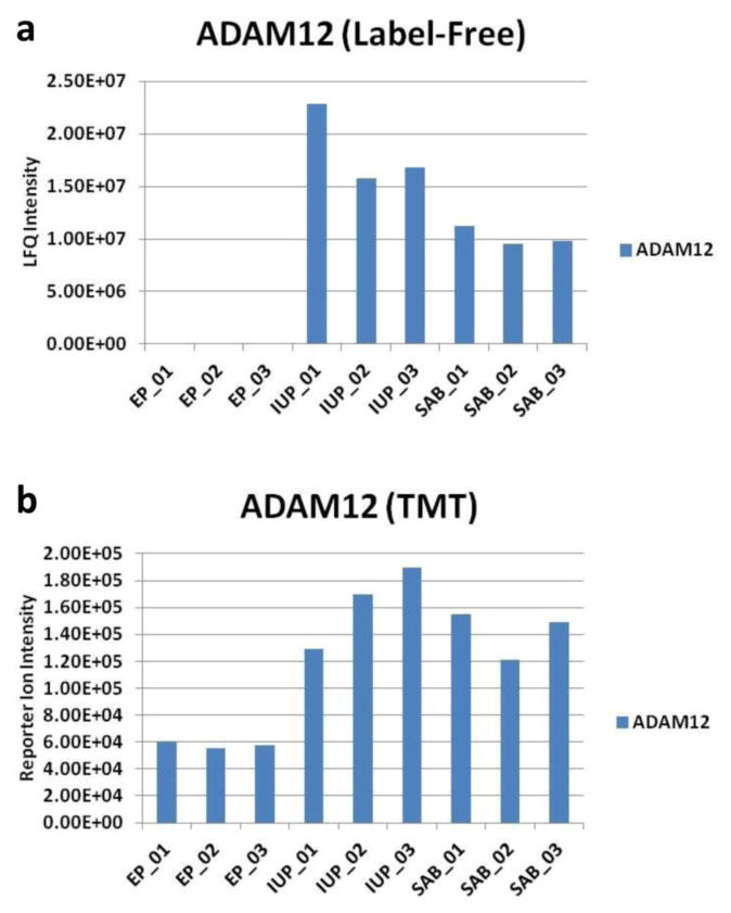
Comparison of label-free and TMT protein quantitation for ADAM12, a known ectopic pregnancy biomarker. (a) Label-free quantitaion of a 4 hr LC-MS/MS run for triplicate depletions using IGY14-Supermix columns of pooled plasma from individuals having an ectopic pregnancy (EP), normal intrauterine pregnancy (IUP), or spontaneous abortion (SAB). Normalized LFQ protein intensity for ADAM12 is shown. (b) 10-plex TMT labeling of the same triplicate pooled plasma samples. Summed intensities of measured peak m/z values for the TMT reporter ions representing ADAM12 are shown.
Fig. 2.
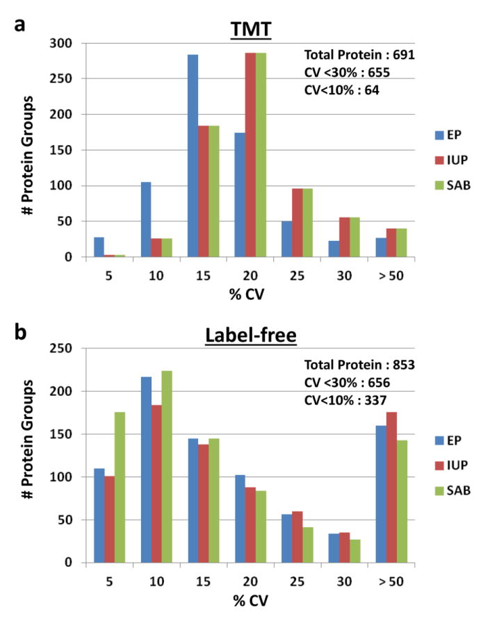
Coefficients of variation of protein identifications for a comparison of label-free and TMT quantitation. (a) 10-plex TMT labeling of pools of EP, IUP, and SAB plasma that were depleted in triplicate using IGY14-Supermix columns. (b) Label-free quantitation of the same triplicate pooled plasma samples. “Total Protein” values indicated represent numbers of protein groups across all samples identified by 2 or more peptides and with peptide and protein FDR of 1%. “CV <30% or <10%” values represent averages of the three groups of samples (EP, IUP, SAB).
While single TMT experiments are similar to label-free quantitation methods, the number of proteins consistently quantitated across multiple TMT experiments are greatly reduced as noted above. Due to this limitation we further explored the feasibility of using a modified label-free proteome analysis method to increase depth of analysis in plasma. Although use of isobaric tags can greatly reduce mass spectrometer time for any given level of fractionation compared with label-free quantitation, the missing values across TMT experiments and reduced reliability of quantitation for low abundance proteins at least partially offsets the advantages of multiplexing.
The following protocol describes an in-depth label-free analysis of human plasma samples with MaxQuant. MaxQuant is a freely available software program which uses its own search engine, Andromeda, to search and analyze high-resolution LC-MS/MS data[23,24]. While the software was primarily developed for analysis of stable isotope labeling with amino acids in cell culture (SILAC) data, MaxQuant also employs the MaxLFQ algorithm for label-free quantitation[25]. In the analysis described herein, three different plasma pools were depleted in triplicate with the IgY 14/SuperMix tandem immunoaffinity columns followed by 1D-SDS PAGE, trypsin digestion (for complete protocol, see chapter XX in this book), and label-free quantitation with MaxQuant. For a similar detailed protocol for MaxQuant quantitation of SILAC datasets, see References [26,27].
2 Materials
2.1 Hardware Requirements
Intel Pentium III/800 MHz or higher (or compatible); a dual core processor is recommended.
2 GB RAM per thread that is executed in parallel is required.
There is no upper limit on the number of cores; however a multi-core processor operating on a shared memory machine will maximize the parallelization capabilities of the software [26] .
2.2 Software and Other Requirements
NET framework 4.5 or higher (downloadable from Microsoft).
MSFileReader (downloadable from Thermo Fisher Scientific).
64-bit Windows operating system (Supported versions: Vista SP2, Windows 7, Windows 8, Windows Server 2008, and Windows Server 2012).
MaxQuant Software, version 1.5.2.8 or higher (freely available at www.maxquant.org).
FASTA Sequence Database (e.g. Human Uniprot Database, downloadable from www.uniprot.org).
3 Methods
Unless otherwise noted, the following parameters used for label-free quantitation rely on the default settings in MaxQuant which have been optimized by the developers and are appropriate for most label-free experiments. A more detailed description of these and other parameters, including the Andromeda search configuration, can be found in Reference [26].
3.2 MaxQuant: Raw Files Tab
Load. raw. files. (All .raw files to be analyzed should be stored in the same folder).
Define Experiments (see Note 1).
Define Fractions (see Note 2).
Define Parameter Groups (see Note 3).
3.3 Maxquant: Group Specific Parameters Tab
Select “General” tab.
Set Type: select Standard for label-free quantitation (see Note 4).
Set Multiplicity: select 1 for label-free quantitation (see Note 5).
Set Variable modifications (e.g. methionine oxidation and protein N-terminal acetylation).
Specify Digestion mode and Enzyme used (e.g. “ Specific” and “Trypsin/P” for full-tryptic cleavage constraints).
Set max. # of missed cleavages: default = 2.
Set Match type: Match from and to.
Select “Instrument” tab.
Choose instrument used (e.g. Thermo Fisher Orbitrap, Bruker Q-TOf, AB Sciex Q-TOF). The default parameters will change accordingly based on the instrument selected.
Select “Label-free quantification” tab.
Set Label-free quantitation: select LFQ.
Set the LFQ min. ratio count to 1 (see Note 6).
Keep “Fast LFQ” enabled (see Note 7).
Select “Advanced” tab.
Set the max. number of modifications per peptide: default = 5.
3.4 MaxQuant: Global Parameters Tab
Select “General” tab.
Load a FASTA database file, which has been previously configured in Andromeda (see Note 8).
Set “Fixed modifications” (e.g. carbamidomethyl cysteine).
If appropriate, enable “Match between runs” (see Note 9).
Set the Match time window and Alignment time windows to 0.7 min and 10 min, respectively (see Note 10).
-
Select “Sequences” tab. Parameters include:
Decoy mode: e.g. Revert (reversed sequences)
Special AAs: e.g. KR
Include contaminants: enable (see Note 11).
Select “Identification” tab: keep default settings for a protein and peptide false discovery rate (FDR) of 1% (see Note 12).
-
Select “Protein quantification” tab. Parameters include:
Min. ratio count: 2 (Only applies to SILAC labeling).
Peptides for quantification: Unique + razor (See Note 13).
Enable “Use only unmodified peptides and (e.g. methionine oxidation and N-terminal acetylation), and “Discard unmodified counterpart peptide” features.
Select “Label free quantification” tab.
If more than one parameter group is used, and LFQ normalizations are to be kept separate (see Note 3), enable “Separate LFQ in parameter groups”.
Keep default “Stabilize large LFQ ratios”, “Require MS/MS for LFQ comparisons” and “Advanced site intensities” settings enabled.
-
Other Global Parameters Tabs: (Default settings are suitable for most experiments).
Tables
AIF
MS/MS-FTMS
MS/MS-ITMS
MS/MS-TOF
MS/MS-Unknown
Advanced
3.5 MaxQuant: Performance Tab
In the footer of the program, set the number of parallel threads (physical cores) to be used (see Note 14).
Press “Start”. The completed and ongoing processes can be monitored on the Performance page by selecting the “Show all activities” tab.
When the analysis is complete several output files, including the ProteinGroups.txt and Peptided.txt files, will be available within the “combined/txt” folder located in the same folder where the raw files are stored (see note 15).
Notes
The Experiment column allows you to specify which raw files should be quantified together and which should be kept separate. For example, in an experiment with conditions A, B, and C, where each condition has three replicate runs, by designating the experiments as “A”, “B” and “C”, all intensities for a given protein will be summed for each condition, and three protein intensities will be reported. On the other hand, replicates may be analyzed separately by giving them nine different experiment names, i.e. A1, A2, A3, B1, B2, etc., and nine protein intensities will be reported. Protein intensities can then be summed for each condition manually or within Perseus software post-analysis. We prefer to treat every sample separately and then perform post analysis processing such as averaging replicates in Excel.
This column is annotated when pre-fractionation (e.g. 1-D PAGE, SCX, high pH separations, etc.) and multiple LC-MS/MS analyses per proteome have been done. Specifying fractions is important if you use the “match between runs” feature (See Note 9). Identifications will be matched between all raw files with the same or adjacent fraction numbers.
Parameter Groups are specified when fundamentally different parameters are to be used, e.g. some files may have been from a phosphoproteome analysis and others may have been from a standard proteome analysis. By setting different parameter groups, all data can be analyzed together, choosing appropriate settings for each condition. Parameter groups can be applied to LFQ analyses where a number of files are to be processed together but the experiments are very different from one another, and therefore the underlying assumption of the LFQ algorithm (that for the most part, all samples are similar) does not hold true. When activated, all LFQ normalizations and quantitations will only be done within each parameter group, but the same protein groups will be present across all samples.
“Standard” is appropriate for label-free quantitation. Other options include: “Reporter ion MS2” or “Reporter ion MS3” for TMT or iTRAQ labeled experiments.
“Multiplicity 1” indicates that no label was used. Multiplicitiy 2 or 3 are to be selected when two or three light, medium, or heavy labels are used, such as with SILAC experiments.
MaxQuant quantitates protein levels by computing pair-wise ratios of all common peptides occurring in any two samples within an experiment, and then using the median of peptide ratios as the pair-wise protein ratio. All pair-wise protein ratios are calculated between any two samples within an experiment to achieve the maximum possible protein quantitation information, and resulting protein ratios are ultimately used to determine LFQ intensity profiles [25]. The LFQ minimum ratio count allows the user to define the minimum number of peptides that has to be available in pair-wise comparisons between two samples. The default setting requires 2 common peptides to be present between any two samples in an experiment. If less peptides are present, the ratio between these two samples is not used for the determination of the LFQ intensities. However, this does not necessarily mean that the LFQ intensities for these two samples are not calculated since they might be inferred from other pair-wise sample comparisons. We generally change this setting to 1 to preserve quantitation between samples for proteins that have been identified by 2 or more peptides somewhere in the dataset, but where individual peptides were identified with low intensity and stocastically. After the MaxQuant search is complete, we typically remove low confidence identifications where all samples are identified by only a single peptide.
“Fast-LFQ” is the high-speed version of MaxQuant that uses a meaningful subset of comparisons to determine the normalization factors for each LC-MS run, and hence significantly reduces computational time[25]. This feature is recommended when LFQ is being applied to large numbers of samples (i.e. more than ten different “Experiment” names). If less than ten experiments are being compared, the standard LFQ normalization algorithm is automatically used.
For more details regarding Andromeda configuration, see [26].
When “match between runs” is enabled, identifications are transferred to non-sequenced or non-identified MS features in other LC-MS runs that match identified peptides in one or more runs. [28]. The prerequisite for matching identifications is that the peptides have the same mass within the mass tolerance (ppm) of the identified partner, and the peptides elute at the same point in the gradient within the 0.7 min match time window tolerance (see note 10).
The “alignment time window” is the time window that is used in retention time alignment to search for the best alignment function. The default setting is 20 min, however, we typically reduce this value to 10 min for analyses where mass spectrometer, HPLC, and autoinjector performances were carefully monitored to maintain consistent retention times between all runs. The “match time window” is the time window allowed during “match between runs” for the transfer of peptide identifications and accounts for potential retention time shifts after the retention time alignment has been performed; hence, a narrow window (<1 min, typically 0.7 min) is optimal to minimize false matches of peptides across runs
MaxQuant provides a contaminants.fasta database file within the software that is automatically added to the list of proteins for the in-silico digestion when this feature is enabled. The contaminants database is located in the conf/contaminants.fasta file within the folder containing the MaxQuant executable files. It is recommended to closely look at the contaminants file before performing database searches. We have found that this file contains many bovine serum proteins which are appropriate contaminants for cell lysate experiments using fetal calf serum. However, a few of these bovine proteins can have high homology to human plasma proteins and can result in true identifications being flagged as contaminants when analyzing plasma proteomes, e.g. actin. Therefore, we replace the MaxQuant contaminants.fasta file with our own list of commonly observed keratin and trypsin contaminants and in the case of cell culture, with a more restricted bovine serum list.
FDR is specified at the peptide spectrum match (PSM) and protein level, as determined by the target-decoy approach[29]. The default values are 0.01 (1%), however they may be increased to relax stringency.
This selection will calculate protein ratios using both unique peptides and razor peptide intensities, Razor-peptides are non-unique peptides and these are assigned to the protein group containing the largest number of other peptides, according to Occam's razor principle.
The number of threads refers to the number of physical computer processing cores. Each raw file will be analyzed by one core and the use of multiple cores will considerably reduce analysis times. However, if all available cores are being used for a MaxQuant analysis, any other computational processes running on the computer will be slowed down. Therefore, for large datasets, a dedicated multi-core processor operating on a shared memory machine is recommended[27].
The ProteinGroups.txt file includes information on the identified protein groups in the processed raw-files. Each row contains the group of proteins that could be reconstructed from a set of peptides. Raw and normalized intensities can be observed in the “Intensity” and “LFQ Intensity” columns, respectively (Fig. 3).
Fig. 3.
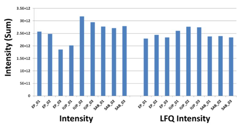
Summed protein intensities for all protein groups before (Intensity, left) and after (LFQ Intensity, right) normalization. Single 4h LC-MS runs of triplicate pools of IGY14-Supermix depleted EP, IUP, and SAB plasma were quantitated in a label-free analysis using MaxQuant, with “match between runs” enabled.
Acknowledgments
This work was supported by NIH Grants RO1HD076279, RO1CA131582, and WW Smith Charitable Trust Grants H1205 and H1305 (D.W. Speicher), PA Department of Health Commonwealth Universal Research Enhancement (CURE) Program Grant (B. Ky), as well as CA10815 (NCI core grant to the Wistar Institute).
References
- 1.Anderson NL, Anderson NG. The human plasma proteome: history, character, and diagnostic prospects. Mol Cell Proteomics. 2002;1(11):845–867. doi: 10.1074/mcp.r200007-mcp200. [DOI] [PubMed] [Google Scholar]
- 2.Jacobs JM, Adkins JN, Qian WJ, Liu T, Shen Y, Camp DG, 2nd, Smith RD. Utilizing human blood plasma for proteomic biomarker discovery. J Proteome Res. 2005;4(4):1073–1085. doi: 10.1021/pr0500657. [DOI] [PubMed] [Google Scholar]
- 3.Hoffman SA, Joo WA, Echan LA, Speicher DW. Higher dimensional (Hi-D) separation strategies dramatically improve the potential for cancer biomarker detection in serum and plasma. J Chromatogr B Analyt Technol Biomed Life Sci. 2007;849(1-2):43–52. doi: 10.1016/j.jchromb.2006.10.069. doi:S1570-0232(06)00885-3 [pii] 10.1016/j.jchromb.2006.10.069. [DOI] [PubMed] [Google Scholar]
- 4.Gulcicek EE, Colangelo CM, McMurray W, Stone K, Williams K, Wu T, Zhao H, Spratt H, Kurosky A, Wu B. Proteomics and the analysis of proteomic data: an overview of current protein-profiling technologies. Curr Protoc Bioinformatics. 2005;Chapter 13(Unit 13):11. doi: 10.1002/0471250953.bi1301s10. [DOI] [PMC free article] [PubMed] [Google Scholar]
- 5.Geyer PE, Kulak NA, Pichler G, Holdt LM, Teupser D, Mann M. Plasma Proteome Profiling to Assess Human Health and Disease. Cell Syst. 2016;2(3):185–195. doi: 10.1016/j.cels.2016.02.015. doi:S2405-4712(16)30072-2 [pii] 10.1016/j.cels.2016.02.015. [DOI] [PubMed] [Google Scholar]
- 6.Sandberg A, Branca RM, Lehtio J, Forshed J. Quantitative accuracy in mass spectrometry based proteomics of complex samples: the impact of labeling and precursor interference. J Proteomics. 2014;96:133–144. doi: 10.1016/j.jprot.2013.10.035. doi:S1874-3919(13)00550-2 [pii] 10.1016/j.jprot.2013.10.035. [DOI] [PubMed] [Google Scholar]
- 7.Thompson A, Schafer J, Kuhn K, Kienle S, Schwarz J, Schmidt G, Neumann T, Johnstone R, Mohammed AK, Hamon C. Tandem mass tags: a novel quantification strategy for comparative analysis of complex protein mixtures by MS/MS. Anal Chem. 2003;75(8):1895–1904. doi: 10.1021/ac0262560. [DOI] [PubMed] [Google Scholar]
- 8.Ross PL, Huang YN, Marchese JN, Williamson B, Parker K, Hattan S, Khainovski N, Pillai S, Dey S, Daniels S, Purkayastha S, Juhasz P, Martin S, Bartlet-Jones M, He F, Jacobson A, Pappin DJ. Multiplexed protein quantitation in Saccharomyces cerevisiae using amine-reactive isobaric tagging reagents. Mol Cell Proteomics. 2004;3(12):1154–1169. doi: 10.1074/mcp.M400129-MCP200. M400129-MCP200 [pii] [DOI] [PubMed] [Google Scholar]
- 9.Wuhr M, Haas W, McAlister GC, Peshkin L, Rad R, Kirschner MW, Gygi SP. Accurate multiplexed proteomics at the MS2 level using the complement reporter ion cluster. Anal Chem. 2012;84(21):9214–9221. doi: 10.1021/ac301962s. [DOI] [PMC free article] [PubMed] [Google Scholar]
- 10.Houel S, Abernathy R, Renganathan K, Meyer-Arendt K, Ahn NG, Old WM. Quantifying the impact of chimera MS/MS spectra on peptide identification in large-scale proteomics studies. J Proteome Res. 2010;9(8):4152–4160. doi: 10.1021/pr1003856. [DOI] [PMC free article] [PubMed] [Google Scholar]
- 11.Old WM, Meyer-Arendt K, Aveline-Wolf L, Pierce KG, Mendoza A, Sevinsky JR, Resing KA, Ahn NG. Comparison of label-free methods for quantifying human proteins by shotgun proteomics. Mol Cell Proteomics. 2005;4(10):1487–1502. doi: 10.1074/mcp.M500084-MCP200. doi:M500084-MCP200 [pii] 10.1074/mcp.M500084-MCP200. [DOI] [PubMed] [Google Scholar]
- 12.America AH, Cordewener JH. Comparative LC-MS: a landscape of peaks and valleys. Proteomics. 2008;8(4):731–749. doi: 10.1002/pmic.200700694. [DOI] [PubMed] [Google Scholar]
- 13.Bantscheff M, Schirle M, Sweetman G, Rick J, Kuster B. Quantitative mass spectrometry in proteomics: a critical review. Anal Bioanal Chem. 2007;389(4):1017–1031. doi: 10.1007/s00216-007-1486-6. [DOI] [PubMed] [Google Scholar]
- 14.Bantscheff M, Lemeer S, Savitski MM, Kuster B. Quantitative mass spectrometry in proteomics: critical review update from 2007 to the present. Anal Bioanal Chem. 2012;404(4):939–965. doi: 10.1007/s00216-012-6203-4. [DOI] [PubMed] [Google Scholar]
- 15.Li Z, Adams RM, Chourey K, Hurst GB, Hettich RL, Pan C. Systematic comparison of label-free, metabolic labeling, and isobaric chemical labeling for quantitative proteomics on LTQ Orbitrap Velos. J Proteome Res. 2012;11(3):1582–1590. doi: 10.1021/pr200748h. [DOI] [PubMed] [Google Scholar]
- 16.Megger DA, Pott LL, Ahrens M, Padden J, Bracht T, Kuhlmann K, Eisenacher M, Meyer HE, Sitek B. Comparison of label-free and label-based strategies for proteome analysis of hepatoma cell lines. Biochim Biophys Acta. 2014;1844(5):967–976. doi: 10.1016/j.bbapap.2013.07.017. doi:S1570-9639(13)00289-6 [pii] 10.1016/j.bbapap.2013.07.017. [DOI] [PubMed] [Google Scholar]
- 17.Patel VJ, Thalassinos K, Slade SE, Connolly JB, Crombie A, Murrell JC, Scrivens JH. A comparison of labeling and label-free mass spectrometry-based proteomics approaches. J Proteome Res. 2009;8(7):3752–3759. doi: 10.1021/pr900080y. [DOI] [PubMed] [Google Scholar]
- 18.Schulze WX, Usadel B. Quantitation in mass-spectrometry-based proteomics. Annu Rev Plant Biol. 2010;61:491–516. doi: 10.1146/annurev-arplant-042809-112132. [DOI] [PubMed] [Google Scholar]
- 19.Karp NA, Huber W, Sadowski PG, Charles PD, Hester SV, Lilley KS. Addressing accuracy and precision issues in iTRAQ quantitation. Mol Cell Proteomics. 2010;9(9):1885–1897. doi: 10.1074/mcp.M900628-MCP200. doi:M900628-MCP200 [pii] 10.1074/mcp.M900628-MCP200. [DOI] [PMC free article] [PubMed] [Google Scholar]
- 20.Ow SY, Salim M, Noirel J, Evans C, Rehman I, Wright PC. iTRAQ underestimation in simple and complex mixtures: “the good, the bad and the ugly”. J Proteome Res. 2009;8(11):5347–5355. doi: 10.1021/pr900634c. [DOI] [PubMed] [Google Scholar]
- 21.Ting L, Rad R, Gygi SP, Haas W. MS3 eliminates ratio distortion in isobaric multiplexed quantitative proteomics. Nat Methods. 2011;8(11):937–940. doi: 10.1038/nmeth.1714. doi:nmeth.1714 [pii] 10.1038/nmeth.1714. [DOI] [PMC free article] [PubMed] [Google Scholar]
- 22.Beer LA, Tang HY, Sriswasdi S, Barnhart KT, Speicher DW. Systematic discovery of ectopic pregnancy serum biomarkers using 3-D protein profiling coupled with label-free quantitation. J Proteome Res. 2011;10(3):1126–1138. doi: 10.1021/pr1008866. [DOI] [PMC free article] [PubMed] [Google Scholar]
- 23.Cox J, Mann M. MaxQuant enables high peptide identification rates, individualized p.p.b.-range mass accuracies and proteome-wide protein quantification. Nat Biotechnol. 2008;26(12):1367–1372. doi: 10.1038/nbt.1511. doi:nbt.1511 [pii] 10.1038/nbt.1511. [DOI] [PubMed] [Google Scholar]
- 24.Cox J, Neuhauser N, Michalski A, Scheltema RA, Olsen JV, Mann M. Andromeda: a peptide search engine integrated into the MaxQuant environment. J Proteome Res. 2011;10(4):1794–1805. doi: 10.1021/pr101065j. [DOI] [PubMed] [Google Scholar]
- 25.Cox J, Hein MY, Luber CA, Paron I, Nagaraj N, Mann M. Accurate proteome-wide label-free quantification by delayed normalization and maximal peptide ratio extraction, termed MaxLFQ. Mol Cell Proteomics. 2014;13(9):2513–2526. doi: 10.1074/mcp.M113.031591. doi:M113.031591 [pii] 10.1074/mcp.M113.031591. [DOI] [PMC free article] [PubMed] [Google Scholar]
- 26.Tyanova S, Mann M, Cox J. MaxQuant for in-depth analysis of large SILAC datasets. Methods Mol Biol. 2014;1188:351–364. doi: 10.1007/978-1-4939-1142-4_24. [DOI] [PubMed] [Google Scholar]
- 27.Cox J, Matic I, Hilger M, Nagaraj N, Selbach M, Olsen JV, Mann M. A practical guide to the MaxQuant computational platform for SILAC-based quantitative proteomics. Nat Protoc. 2009;4(5):698–705. doi: 10.1038/nprot.2009.36. doi:nprot.2009.36 [pii] 10.1038/nprot.2009.36. [DOI] [PubMed] [Google Scholar]
- 28.Geiger T, Wehner A, Schaab C, Cox J, Mann M. Comparative proteomic analysis of eleven common cell lines reveals ubiquitous but varying expression of most proteins. Mol Cell Proteomics. 2012;11(3):M111. doi: 10.1074/mcp.M111.014050. doi:014050. doi:M111.014050 [pii] 10.1074/mcp.M111.014050. [DOI] [PMC free article] [PubMed] [Google Scholar]
- 29.Elias JE, Gygi SP. Target-decoy search strategy for mass spectrometry-based proteomics. Methods Mol Biol. 2010;604:55–71. doi: 10.1007/978-1-60761-444-9_5. [DOI] [PMC free article] [PubMed] [Google Scholar]