Virtual Spirometry and Activity Monitoring using Multi-channel Electrical Impedance Plethysmographs in Ambulatory Settings

Abstract

Continuous monitoring of respiratory patterns and physical activity levels can be useful for remote health management of patients with conditions such as heart disease and chronic obstructive pulmonary disease (COPD). In a clinical setting, spirometers serve as the gold-standard for monitoring respiratory patterns such as breathing-rate and changes in lung-volume. However, direct measurements using a spirometer requires placement of a sensor in the patient’s airway and is thus infeasible for continuous monitoring in non-clinical, ambulatory settings. Under these conditions, indirect respiration monitoring using electrical impedance plethysmographs (EIP) is more suitable but are susceptible to motion artifacts. In this paper we investigate whether multi-channel EIP can be used to perform virtual spirometry under ambulatory settings. The experiments presented in this paper are based on preliminary data collected from 19 adult human subjects under realistic ambulatory and non-ambulatory settings. We first highlight the salient features of the signal acquired from a standard spirometer. We then compare the performance of different bio-signal processing algorithms in estimating the spirometer signal using multiple EIP sensors and in the presence of motion artifacts and real-world interferences. We demonstrate that in addition to reliably determining different respiratory patterns and states, multi-channel EIP could also be used to reliably extract information regarding different patient physical activity states like bending or stretching.

I. Introduction

DIFFICULTY in breathing and shortness of breath are early indicators of deteriorating conditions in patients suffering from chronic obstructive pulmonary disease (COPD) or heart failure (HF). In patients with these pathologies, tachypnea, or an increase in breathing-rate could signify an attempt by the body to compensate for poor pulmonary gas exchange and/or poor cardiac circulation. This biomarker has been used as an early warning predictor of cardiac arrests under ICU conditions [1]. Similarly, COPD exacerbations are often accompanied by symptoms such as increased dyspnea or shortness of breath [2]. Thus, in HF and COPD patients, monitoring abnormal changes in respiratory patterns could facilitate early clinical interventions by caregivers and hence could potentially save lives. Unfortunately, spirometry which is the current gold-standard for monitoring respiratory patterns is limited to only non-ambulatory clinical settings. This is because of several factors such as: its invasive nature and related patient discomfort, the size of the accompanying equipment, and the difficulty in administering the equipment.

An alternative but a more suitable approach for ambulatory settings is to use an indirect technique such as Electrical Impedance Plethsmography (EIP) which measures the breathing patterns using sensors attached directly over the torso. EIP is routinely used for post-surgical monitoring of electrocardiogram (ECG) signals in patients suffering from heart disease and the emergence of portable EIP systems [3], [4] has opened the possibility that EIP technology could be used for monitoring patients in non-clinical settings. However, the key obstacle that is preventing widespread adoption of EIP in ambulatory environments is its susceptibility to motion artifacts during periods of physical activity and exertion. Even seemingly gentle events such as arm motion can completely distort the respiratory pattern obtained using EIP. One of the hypothesis of this paper is that the interference due to motion artifacts could be reduced, to some extent, using multiple EIP channels, each acquiring information that is spatially diverse with respect to each other. In this paper we investigate different multi-channel biosignal processing algorithms that can extract high-quality respiratory patterns from a mixture of signal outputs from different EIP channels, obtained under non-clinical, ambulatory settings. We demonstrate that multichannel EIP in conjunction with proper post-processing results in a reasonable estimate of the spirometer output. As a result, the proposed technology could be used to implement virtual spirometry (using multi-channel EIP) as shown in Fig. 1, without using an actual spirometer, also shown in Fig. 1.

Fig. 1.

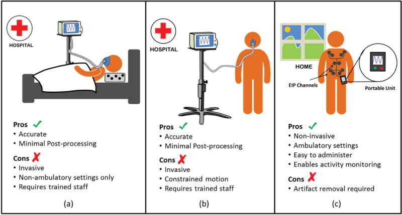
Conventional spirometry using a flowmeter (a) and (b); versus virtual spirometry using multi-channel EIPs (c).

Prior work in this area of have mainly focussed on reducing the effect of motion artifacts. For instance, in [5]–[7] an independent component analysis (ICA) was employed to extract respiratory information from multi-channel EIP. ICA assumes linear mixing of independent components which may not be valid under all circumstances. In [8] ε-tube filtering is employed to eliminate motion artifacts from the EIP signal. Results demonstrated better performance than ICA; however, this model was limited to only large-amplitude artifacts that were introduced under normal breathing conditions. Other related work [9]–[12] focus on estimation of only breathing rate and employ data collected from non-ambulatory human subjects lying in a supine position. In this paper we focus on cases that include both ambulatory and non-ambulatory conditions. We have collected preliminary data from human-subjects who were instructed to simulate a number of respiratory states such as apnea, tachypnea, coughing, shallow breathing and hyperventilation. We then experimented with a number of standard, supervised learning techniques for estimating the spirometer signal from the multi-channel EIPs. Once the spirometer signal could be reliably estimated using this technique, several clinically relevant parameters such as breathing-rate or lung-volume could be determined using basic post-processing techniques. In addition to accomplishing virtual spirometry, we also demonstrate that it is possible to classify different physical activities (PAs) using the time-frequency signatures of the signal traces due to motion artifacts. In this regard, the EIP-based activity signatures could be used in conjunction with existing approaches that use accelerometers or gyroscopes [13]–[17] to improve the classification performance of existing PA systems.

This paper is organized as follows: section II discusses some of the salient characteristics of spirometry and EIP and how they may be exploited to obtain an accurate estimate of the spirometer signal. The data collection protocol is presented in section II-A. Some regression techniques for estimating the spirometer output from EIP channel outputs are discussed in section III. These include: support vector regression, Gaussian mixture regression and DCT based regression. Section IV describes the Segregated Envelope and Carrier (SEC) estimation algorithm. This algorithm assumes that (in a small time window) the spirometer output can be approximated by an amplitude modulated signal. The amplitude and carrier (breathing rate) are estimated separately and then multiplied to obtain the spirometer signal. Spirometry results for the various techniques are presented in section V. Physical activity classification based on time-frequency signatures of the underlying motion artifacts is discussed in section VI. Activity classification results are presented in section VII. Conclusions are presented in section VIII.

II. Salient Characteristics of Spirometry and EIP

EIP is based on measuring changes in electrical impedance across two electrodes using a low-amplitude, high-frequency alternating current that is injected into the body and across a pair of electrodes [19]. When the pair of electrodes is placed over the torso, the output signal varies in direct proportion to the volume of air inspired and expired from the lungs during breathing. This signal thus has a significant correlation with the output from a spirometer which consists of a mouthpiece that directly measures the airflow in the lungs during inspiration and expiration [18]. Fig. 2 shows the output of a spirometer and the corresponding outputs from multiple EIP channels in the presence of different motion artifacts and under different respiratory conditions. During interval-(a) the subject is reaching for an object while breathing normally (as indicated by the spirometer output) in a seated position. Notice, the motion artifacts in the EIP channels; the spirometer output is unaffected. During intervals-(b) through (e) the subject is laying face-up on a bed and maintaining different respiratory-states, each for a duration of approximately 30 seconds. EIP channels or (different pair of electrodes) measure lung volume directly resulting in low amplitude outputs during tachypnea (or shallow fast breathing) regions. This implies that in noisy conditions it could be challenging to differentiate between tachypnea and apnea regions.

Fig. 2.

Reference Spirometer signal and corresponds (filtered) EIP channel outputs under different motion and breathing conditions (a) reaching for object; (b) Tachypnea (shallow fast breathing); (c) Hyperventilation (deep fast breathing); (d) deep slow breathing; (e) Apnea (holding breath).

Since our objective is to estimate the spirometer output based on the EIP channels, we examine the time-frequency characteristics of the spirometer output to highlight the important information in this signal. This information must be estimated accurately in order to produce a high-quality approximation of the spirometer output. The frequency spectrum of the spirometer output consists of one dominant harmonic which corresponds to the breathing-rate. However, a spirometer’s time-domain waveform is not a pure harmonic implying the presence of other artifacts introduced by the biomechanics of respiration. To understand the contribution of these harmonics we perform a very basic spectral analysis of the spirometer output, using the Discrete Cosine Transform (DCT). The DCT is known for its “Energy Compaction” property [20] and if the analysis results in a sparse representation then it would imply that we would need to estimate a relatively small number of parameters in order to produce a high-quality estimate of the spirometer signal. The spirometer output, y, is divided into non-overlapping time-windows of length (M) equal to 200 samples each (Note: spirometer sampling rate = 40 samples/sec). Samples y_i from any given time-window i are transformed using the DCT basis to obtain the coefficient vector z_i as below:

$${\mathbf{z}}_i=\mathbf{T}{\mathbf{y}}_i\text{for}i=[1,\dots ,F]$$ (1)

here, T represents the (M × M) DCT basis and F is the total number of non-overlapping time-windows in the spirometer output y. The DCT coefficients are sorted and the M – P coefficients with the smallest amplitudes are set to zero. The coefficients are then reordered and put in the (M × 1) vector ${\stackrel{\sim }{\mathbf{z}}}_i$ which contains P(< M) nonzero values; corresponding to the largest amplitude harmonics of y_i and M − P zeros. After this a quantized version of the spirometer signal is obtained via the inverse DCT transform

$${\stackrel{\sim }{\mathbf{y}}}_i={\mathbf{T}}^{-1}{\stackrel{\sim }{\mathbf{z}}}_i\text{for}i=[1,\dots ,F]$$ (2)

The number of non-zero coefficients (P) in ${\stackrel{\sim }{\mathbf{z}}}_i$ is varied from 1 to M and the quality of the reconstructed signal is evaluated by computing its Signal-to-Distortion Ratio (SDR) at each value of P

$${\mathrm{SDR}}_P=\frac{1}{F}{\displaystyle \sum _{i=1}^{F}20\log \frac{\Vert {\stackrel{\sim }{\mathbf{y}}}_i\Vert }{\Vert {\mathbf{y}}_i-{\stackrel{\sim }{\mathbf{y}}}_i\Vert }}\text{for}P=[1,\dots ,M]$$ (3)

where, || || represents the l₂-norm. Fig. 3 displays a plot of the Signal-to-Distortion Ratio (SDR), of the spirometer output displayed in Fig. 4 (a), for different values of P. We are primarily interested in the SDR values at small values of P therefore, Fig. 3 displays SDR only upto a maximum of P = 30 coefficients. Fig. 3 indicates that a reasonable SDR (>10 dB) can be achieved even using a small number (10 to 15) of DCT coefficients. Retention of only the largest amplitude coefficient results in a SDR = −0.104 dB, the corresponding quantized signal is shown in Fig. 4 (b). This signal would still enable detection of the breathing-rate however, it is very coarsely quantized and additional parameters such as lung-volume estimation cannot be extracted. As a consequence, the number of non-zero coefficients must be increased if the objective is to obtain a better and clinically relevant estimate of the spirometer output. An alternate strategy could be to approximate the spirometer signal by an amplitude modulated (AM) signal within the sample window of length M. In this approach the carrier (breathing rate) component can be obtained by retaining only the highest amplitude coefficient and setting the remaining M − 1, lower amplitude, coefficients to zero. This single harmonic (or carrier) can then be multiplied with the envelope of the spirometer signal, which is estimated separately. The temporal variation in amplitude of the resulting signal is controlled by the envelope and therefore, prior to multiplication the amplitude of the carrier frequency is set to 1. Application of the AM approximation technique to the spirometer waveform in Fig. 4 (a) results in the waveform shown in Fig. 4. Here the carrier component is obtained by retaining only the largest amplitude DCT coefficient in non-overlapping windows of the spirometer waveform in Fig. 4 (a). The envelope is extracted, from the spirometer waveform, using a simple square-law detector [21]. The SDR in this case is equal to 5.483 dB therefore, resulting in a gain of about 5.5 dB when compared to the single harmonic approach. It can also be seen that the AM approximated signal is very similar to the reference spirometer signal. It is highlighted here that the carrier and envelope in Fig.s 4 (b) and (c) are extracted directly from the spirometer waveform however, this is only for illustrative purposes only. All the approaches discussed in the subsequent sections extract this information from the EIP channels and not from the spirometer waveform.

Fig. 3.

Signal-to-Distortion Ratio of a Spirometer Signal Reconstructed for a fixed number of DCT coefficients.

Fig. 4.

(a) Original Spirometer signal. (b) Reconstructed signal using only 1 DCT coefficient; SDR = −0.104 dB. (c) Reconstructed signal using the AM approximation; SDR = 5.483 dB.

The AM approximation will be utilized in one of the techniques employed for estimation of the spirometer from EIP channels. We call this technique the Segregated Envelop and Carrier (SEC) detection; details are presented in section IV. The regression techniques in this paper employ supervised learning to predict the spirometer output from multiple EIP channel outputs. The output of an EIP channel is more sensitive to changes in impedance of the muscular tissue surrounding the lungs which has higher conductivity than the actual lung tissue. The output signal is therefore, more representative of chest motion than the actual lung airflow and lung volume. As a result patient movements that distort the chest cavity can cause significant motion artifacts. A potential solution to this problem is to employ multiple EIP channels placed at different spatial locations over the patient’s body. Since the respiratory signal is correlated among all the sensors and the patient movements are sporadic and generally not correlated therefore, we should be able to separate the respiratory signal from motion artifacts using a multi-sensor setup. To illustrate the benefit gained by using multiple EIP-electrode sensors we divide the respiratory data into, non-overlapping, segments of equal time duration and then compute the percentage of segments during which the breathing rate obtained from any particular sensor is closest to the reference breathing rate obtained from a spirometer. In this way we can compute that percentage of segments during which a certain sensor gives the best performance (or the smallest breathing rate error). The bar-graph in Fig. 5 plots the percentage of segments during which each of the 10 sensors gives the best performance. It can be observed that there is no clear winner and the most accurate EIP sensor gives the best performance in only about 20% of the total segments. This is not unexpected since the data is not artifact free and the degree of impact of a motion artifact on a sensor depends on the nature of the underlying physical activity and the sensor’s location. For example, a sudden right arm movement is more likely to distort outputs of sensors on the right side of the torso than it is to distort the left side sensors. As a result there seems to be no single sensor that gives the best performance across all the different activities contained in the various segments of data. Therefore, the use of multiple EIP sensors is justified as it enables us to reduce the impact of motion-artifacts on respiratory signal estimation.

Fig. 5.

Percentage of data during which different EIP-channels give the lowest error rate.

A. Data Collection And Pre-processing

Our experiments are based on 19 respiratory datasets each of which was recorded from a distinct adult human subject. A total of 10 EIP channel were placed at different spatial locations on the human subject’s torso as shown in Fig. 6. This spatial layout of EIP channels is based on our previous work [22] and was selected because the differential impedance measured across the multi-lead EIP channels represents the spatially distributed respiratory information along with localized motion artifacts. This spatial diversity is exploited in our proposed algorithms to separate the respiration signal from motion artifacts. A spirometer (Model RX137F Biopac Inc. Goleta, CA) is used as the reference respiratory signal. The spirometer and EIP channels were switched on and off by two different operators and the output signals were aligned manually. Excess pre- and post-samples were truncated. The spirometer and EIP hardware have different sampling rates therefore, interpolation was employed to waveforms to equalize their respective sampling rates.

Fig. 6.

Spatial location of EIP channels on a human subject’s torso during data collection.

For each human subject the average duration of the recorded dataset is about 32 minutes. Data was recorded in 2 minute long sessions i.e.; each subject’s dataset contains around 16 sessions. A session started with the subject breathing normally at rest for about 30 seconds after which he was instructed to perform an activity for a duration of about 30 to 60 seconds. Each dataset contains multiple sessions with 5 distinct physical activities namely: (1) Eating (2) Reaching for object (3) Walking (4) Rolling left to right on bed and (5) Coughing. Sessions containing eating or coughing impact the spirometer output as well and therefore, are considered only during physical activity classification (not for respiratory signal estimation). In addition to physical activities each dataset also contains instances of distinct respiratory states such as: normal breathing, apnea, tachypnea (shallow fast breathing), hyperventilation (deep fast breathing) and slow deep breathing. Sessions containing apnea, tachypnea and hyperventilation are recorded with the subject at rest and therefore, are free from motion artifacts. The output of each EIP-channel was passed through a high-pass filter and a DC blocking filter in order to suppress high frequency noise and the DC-baseline which results from slight shifts in sensor position over time.

III. Spirometer Signal Regression

Our target is to obtain an accurate estimate of the spirometer output using the outputs of the EIP channels. Within the framework of supervised learning this can be formulated as a regression problem where the objective is to learn the mapping from EIP to the spirometer output. For each human subject we first train a learning algorithm on a large proportion of the respiratory dataset. After training, the algorithm is tested on a non-overlapping subset of the data. The spirometer estimate produced using (only) the EIP channels is compared with the reference (true) spirometer signal and performance evaluation metrics are computed. An estimated signal is considered to be high quality if both its frequency and temporal amplitude variations closely resemble the reference spirometer signal. More formally, the following two metrics are employed for performance evaluation:

1) Average Breathing-Rate Error (BR_err)

To evaluate the accuracy of the respiration rate calculated in each frame we calculated difference in breaths-per-minute (BPM) between the reference spirometer signal and the estimated signal. More specifically the input signal is divided into 10 sec frames and the respiration rate is calculated by identifying the highest energy frequency component in the spectrogram. The spectrogram was evaluated using 10 sec long Gaussian windows with an overlap of 5 sec between successive windows. The average breathing rate error (BR_err) is then computed by first taking the “absolute” difference between the reference and estimated breathing-rate curves and then averaging over the total number of frames.

2) Envelope Correlation Coefficient (E_ρ)

In order to gauge how accurately our estimated signal captures the temporal variation of the spirometer’s amplitude we employ the correlation-coefficient as an evaluation metric. More specifically, for each two minute session we first extract the envelopes of the estimated and the corresponding spirometer signal and then evaluate the correlation coefficient between them. This metric is critical for evaluation of test signals that contain a mixture of different respiratory states where the envelope exhibits significant temporal variations (e.g. the signal in Fig. 4).

A. Gini-Support Vector Regression (GiniSVR)

Support vector machines (SVM) [23], [24] are amongst the most popular and widely applied tools in regression problems. For SV regression we employed a variant of SVM called Gini-support vector machines [25]. The dimension, d, of the input feature vectors is equal to 20. Each feature vector contains 10 time samples (one corresponding to each of the 10 channels) and an additional 10 values containing the delta coefficients of the outputs of each channel. The delta coefficients of any time-series correspond to its 1^st derivative and are employed here to capture the temporal dependence on the preceding samples. In order to capture temporal dependence we also, experimented with features based on the auto-regressive (AR) model however, the results were not encouraging and therefore, are not presented here. The parameters of the SVM were selected by performing a grid-search on a large collections of test signals from different patients; the values that gave the best performance (in terms of the performance metrics described above) were selected for the rest of the simulations.

B. Gaussian Mixture Regression (GMR)

Given the harmonic nature of the respiratory signal, a Gaussian Mixture based approach seems to be a very appealing option. For example, Gaussian mixture models (GMMs) are one of the most widely employed methods in speech based applications [26], [27] where the underlying signal contains complex harmonic information. GMMs are based on the assumption that the underlying distribution of the data can be approximated by a multi-modal Gaussian distribution. A single instance of the feature vector, x, at the input of the Gaussian mixture model is d(= 20) dimensional and consists of the channels outputs plus their corresponding delta coefficients. Thus the feature extraction block is identical to the one employed for SVM regression. The Gaussian mixture density of a (d + 1) dimensional multivariate random variable Φ = [x, y], obtained by concatenating x and the (1-dimensional) spirometer output y, is given by [28]:

$$p(\mathbf{\Phi })=p(\mathbf{x},\mathbf{y})={\displaystyle \sum _{k=1}^K{\pi }_k}\mathcal{N}(\mathbf{\Phi };{\mathit{\mu }}_k,{\sum }_k)$$ (4)

where, K is the total number of Gaussian components, π_k are non-negative mixing components with ${\displaystyle {\sum }_{k=1}^K{\pi }_k=1}$ and $\mathcal{N}(\mathbf{\Phi };{\mathit{\mu }}_k,{\sum }_k)$ represents a multi-variate Gaussian density. Furthermore, μ_k denotes the mean vector and is given by:

$${\mathit{\mu }}_k=\left(\begin{array}{c}{\mathit{\mu }}_{k\mathrm{x}}\\ {\mathit{\mu }}_{k\mathrm{y}}\end{array}\right)$$ (5)

Σ_k represents the covariance and is given by:

$${\sum }_k=\left(\begin{array}{cc}{\sum }_{k\mathbf{xx}}& {\sum }_{k\mathbf{xy}}\\ {\sum }_{k\mathbf{yx}}& {\sum }_{k\mathbf{yy}}\end{array}\right)$$ (6)

After initialization using K-means clustering [29] the EM algorithm [30] is employed to find the parameters of the Gaussian mixture distribution(of equation (4)) that best fits the training data. The number of mixture components (K) is determined using the Bayesian-Information Criterion (BIC).

The conditional distribution, p_k(y|x), of a component k, of the spirometer output y given the input feature vector x is determined by dividing the joint distribution, p_k(x, y), by the marginal distribution, p_k(x) [28]:

$$p_k(\mathbf{y}|\mathbf{x})=\frac{p_k(\mathbf{x},\mathbf{y})}{p_k(\mathbf{x})}=\mathcal{N}\left(\mathbf{x}|{\mathit{\mu }}_{k\mathbf{y}|\mathbf{x}},{\mathrm{\Lambda }}_{k\mathbf{yy}}^{-1}\right)$$ (7)

where, Λ_kyy is a submatrix of the matrix ${\mathbf{\Lambda }}_k={\sum }_k^{-1}$ given by:

$${\mathbf{\Lambda }}_k=\left(\begin{array}{cc}{\mathbf{\Lambda }}_{k\mathbf{xx}}& {\mathbf{\Lambda }}_{k\mathbf{xy}}\\ {\mathbf{\Lambda }}_{k\mathbf{yx}}& {\mathbf{\Lambda }}_{k\mathbf{yy}}\end{array}\right)$$ (8)

The conditional mean, μ_ky|x, is given by:

$${\mathit{\mu }}_{k\mathbf{y}|\mathbf{x}}={\mathit{\mu }}_{k\mathbf{y}}-{\mathbf{\Lambda }}_{k\mathbf{yy}}^{-1}{\mathbf{\Lambda }}_{k\mathbf{yx}}(\mathbf{x}-{\mathit{\mu }}_{k\mathbf{x}})$$ (9)

During the test phase the spirometer output is predicted from the feature vectors using the Gaussian mixture distribution learnt during the training phase. More specifically; given a test vector x the estimate ŷ of the spirometer is given by:

$$\widehat{\mathbf{y}}=\mathbb{E}[p(\mathbf{y}|\mathbf{x})]$$ (10)

where, $\mathbb{E}[p(\mathbf{y}|\mathbf{x})]$ represents the expectation of the conditional distribution p(y|x).

C. DCT Based Estimation

We now examine a filtering technique that operates on temporal frames of finite length and estimates the spirometer signal on a frame-by-frame basis, in contrast to the sample-by-sample estimation approach employed by Gini-SVR and GMR. This approach uses simple DCT based filtering and requires no training. The primary motivation for presenting this approach is to use it as a baseline to gauge the performance gains achievable by employing learning algorithms such as SVM and GMM. This approach is similar to the DCT filtering described in equations (1) and (2) except that the spectral harmonics are now extracted from the EIP channels instead of the spirometer output. The output signal from each channel is split into non-overlapping frames of length M temporal samples. Different frame lengths were experimented with; M = 200 samples was found to give the best performance. The maximum number of frames in a given signal is denoted by F. The (M × N) matrix X_i corresponds to the i^th time-window and contains the M samples from the N (=10) EIP channels in its columns. Its corresponding DCT coefficient matrix C_i obtained via the DCT transformation as below:

$${\mathbf{C}}_i=\mathbf{T}{\mathbf{X}}_i\text{for}i=[1,\dots ,F]$$ (11)

where, T represents the (M ×M) DCT basis. In the next step the quantized coefficient matrix ${\stackrel{\sim }{\mathbf{C}}}_i$ is obtained by setting all, but the P largest amplitude coefficients in every column of C_i to zero. The number of non-zero coefficients was determined heuristically. P = 7 gave the best results and thus was used for the results presented here. The mean coefficient vector ${\stackrel{\sim }{\mathrm{x}}}_i$ is then obtained by taking the average over all the EIP channels:

$${\stackrel{\sim }{\mathbf{x}}}_i=\frac{1}{N}{\displaystyle \sum _{n=1}^N{\stackrel{\sim }{\mathbf{c}}}_n^i}$$ (12)

where, ${\stackrel{\sim }{\mathbf{c}}}_n^i$ represents the n^th column of ${\stackrel{\sim }{\mathbf{C}}}_i$; the quantized coefficient matrix. Finally, the spirometer estimate is obtained via the inverse DCT transform:

$${\widehat{\mathbf{y}}}_i={\mathbf{T}}^{-1}{\stackrel{\sim }{\mathbf{x}}}_i\text{for}i=[1,\dots ,F]$$ (13)

IV. Spirometry using SEC Estimation

We now introduce a novel approach titled Segregated Envelope and Carrier (SEC) Estimation. SEC estimation is based on the AM approximation of the spirometer signal discussed in section II. SEC views the spirometer output as an AM signal, albeit with a time varying carrier component. The primary advantage of the AM approximation is that it enables separate evaluation of the envelope and breathing rate thus preventing errors in estimation of parameter from effecting the other. The block diagram of a framework based on the AM approximation is shown in Fig. 7, the Envelope Estimator and the Carrier Estimator blocks provide predictions of the signal’s amplitude and breathing rate respectively. The outputs of both blocks are then multiplied to obtain the the estimated spirometer signal. This approach may also be motivated physiologically in the sense that physical activity by the subject generally introduces large amplitude distortions in the EIP channels while the frequency information (in some, if not all) the channels still remains intact. In such a scenario we may benefit by segregating the estimation of the signal’s rate and envelope. Instead of the sample by sample approach employed in the SVR and GMR, estimation of the signal envelope over a relatively longer temporal window; this may enable mitigation of the large amplitude variations which, in some cases, are observed in the motion artifact regions of the sample by sample approaches. In addition to envelope and carrier estimation block SEC also contains a respiratory state detector whose primary purpose is to detect the onset of an episode of accelerated breathing such as tachypnea or hyperventilation. This is required because accelerated breathing patterns, especially tachypnea, are visible as very low amplitude signals in EIP channel outputs (e.g; see regions (b) and (c) in Fig. 2). As a result they are often confused with low breathing and apnea regions and thus require special care when estimating breathing rate and amplitude. The respiratory state detector alerts the envelope and carrier detection blocks if accelerated breathing region is detected enabling them to adapt their parameters so that accelerated breathing information is not discarded as noise.

Fig. 7.

Block diagram of SEC estimation using the AM approximation.

The envelope estimation block employs regression techniques similar to those used in subsections III-A and III-B with the exception that training is performed using the envelope of the spirometer signal instead of it’s actual sample values. The input features remain that same as those employed in the preceding sections. By focusing solely on the envelope (and not the carrier) we hope that the classifier maybe be able to learn the temporal variations in the signal amplitude with ease.

During the training phase the envelope is obtained by using a square-law detector that is used widely in AM demodulation [21]. Square-law detection works by squaring the AM signal, applying a low-pass filter and then taking the square-root to obtain the envelope (or the modulating) signal. SVM and GMM models are then trained to predict the envelope from the output of the EIP channels. Analysis of SVR and GMR based envelope estimation indicates that for the majority of Test Data, GMR performs better in accelerated breathing regions (tachypnea and hyperventilation) whereas, the SVR is better in normal breathing regions. Therefore, the SEC, envelope is obtained by combining the envelope outputs from the SVR and GMR based envelope estimators. To elaborate, the SVR envelope is employed at normal breathing rates and the GMR envelope is employed at accelerated breathing rates. This switching between GMR and SVR envelopes is based on the decision of the respiratory state detector.

The carrier estimation block obtains an estimate of the breathing rate over a small time window of length M = 200 samples. The extracted breathing frequency is then multiplied with the corresponding output of the envelope estimator (over the same time window) to obtain spirometer signal. For carrier estimation we again employed DCT filtering. The frequency harmonic corresponding to the largest amplitude DCT coefficient of each time-window (of M samples) was selected as the carrier frequency. However, if the largest DCT coefficient corresponds to an accelerated breathing frequency but the respiratory state detector indicates the presence of an apnea region then the carrier frequency is set to zero.

Two types of respiratory state detectors have been tested. The first one employs Periodogram to detect accelerated breathing regions. The second respiratory state detector uses the Discrete-Wavelet-Transform (DWT). These two approaches are now discussed in detail.

A. SEC with Periodogram based Respiratory state detector Detection (SECP)

Welch’s periodogram was employed to detect regions of accelerated breathing. Time intervals where the most dominant frequency lies in the accelerated breathing range and whose power exceeds a threshold ξ are classified as accelerated breathing intervals. The threshold ξ was determined heuristically from data. In case the power is below the threshold and contribution of low-frequency components is also insignificant then the interval is classified as belonging to an apnea region. The high-frequency in this case is most likely due to sensor noise and thus filtered out. The envelope estimator is switched to GMR in case an accelerated breathing interval is detected. Otherwise, an SVR envelope estimator is employed.

B. SEC with Wavelet based Respiratory state Detector (SECW)

The problem with Periodogram based region detection is that it allows uniform resolution in the spectral and temporal domains. Physiological breathing rates correspond to very low frequencies located within a narrow bandwidth. This makes it difficult to design traditional filters that can differentiate between the different frequency bands spanning the physiological frequencies. Wavelet filtering provides an efficient way to achieve high frequency resolution at lower frequency bands. The discrete wavelet transformation (DWT) of a signal length N can be obtain efficiently via multi-resolution analysis (MRA) [32]. The enhanced frequency resolution achieved by the application of DWT can be very useful for differentiating various respiratory states which are located very close to each other in the frequency domain. An illustration of this is presented in Fig. 8 where the top plot contains the output of a single EIP channel during different respiratory states. Daubechies wavelet decomposition coefficients at levels d₃, d₅, d₆ and d₈ are shown in the lower plots. Lower wavelet decomposition levels correspond to higher frequency bands whereas high decomposition levels represent lower frequencies. It can be seen that d₃ coefficients have the highest value in shallow fast breathing (or hyperventilation) regions and are much smaller in normal and slow breathing regions. This means that decomposition coefficients d₃ may be employed to differentiate hyperventilation regions from normal and slow breathing regions. Ideally, d₃ coefficients should be zero in normal and slow breathing regions however, the presence of noise in the sensor output results in non-zero coefficients. Similarly, decomposition coefficients d₅ seems to accurately indicate the presence of Deep fast breathing regions whereas coefficients d₆ and d₈ seem to indicate the presence of normal breathing and deep slow breathing regions or respiratory states.

Fig. 8.

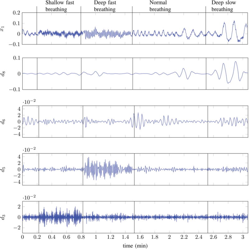
Channel-1 output x₁[n] and its corresponding Daubechies-Wavelet [31] details at different levels.

1) Region Score Computation

The identification of any respiratory state or event should preferably be based on a probabilistic measure as it would enable soft decisions making the overall framework flexible. Fig. 8 demonstrates that different respiratory states are easy to identify at distinct decomposition levels for instance, tachypnea is most easily identifiable at level-3 whereas, slow-deep-breathing lies at level-8. We now construct two probabilistic scores based on the wavelet detail coefficients that enable us to classify different respiratory states. We denote the wavelet detail coefficients corresponding to to level-l of the discrete-time output x_m[n], from channel-m, by d_lm[n]. The first step is to extract the envelope of d_lm[n]:

$$d_{lm}^{\prime }[n]=\text{Envelope}[d_{lm}[n]]$$ (14)

The reason for using the envelope (instead of the sample value of detail coefficient curve) is to capture the slow temporal variations of the curve. Wavelet decomposition is computed up to level-8. The first two levels (Level-1 & Level-2) are discarded since they correspond to high-frequency noise. Upsampling is applied to all wavelet detail coefficients to make them the same length as the input signal x_m[n]. Next, we divide the data, from each subject, into non-overlapping test and reference segments. We ensure that the reference segment contains multiple instances of the human-subject under a number of different respiratory states. After this a distance measure r_lm[n] is evaluated as below:

$$r_{lm}[n]=d_{lm}^{\prime }[n]-{\mu }_{lm}$$ (15)

Here, μ_lm denotes the expected value of $d_{lm}^{\prime }[n]$ in the reference, or training, segments. r_lm[n] indicates the variation of the (envelope of) wavelet detail-l (of sensor-m) above or below its average value in the training segments. The logistic function is then applied to convert r_lm[n] into a probabilistic measure:

$$p_{lm}[n]=\frac{1}{1+\mathit{exp}\left(-c{r}_{lm}[n]\right)}$$ (16)

where, c is a constant; it controls the saturation characteristics of the logistic curve¹. Positive values of r_lm[n] are mapped to p_lm[n] ∈ (0.5, 1] whereas negative values result in p_lm[n] ∈ [0, 0.5). p_lm[n] = 0.5 when r_lm[n] = 0. As demonstrated in Fig. 8 the high or accelerated breathing rates are found in levels 3 and 4. Therefore, we compute the probability, $p_m^{\prime }[n]$, that a sample, at time n from channel-m, belongs to an accelerated respiratory state as below:

$$p_m^{\prime }[n]=\frac{1}{2}\left(p_{3m}[n]+p_{4m}[n]\right)$$ (17)

Similarly, the probabilities from levels 5 to 8 are combined to obtain the the probability of sample n, from channel-m, belonging to a normal (or low) breathing state:

$${\overline{p}}_m[n]=\frac{1}{4}{\displaystyle \sum _{l=5}^8{p}_{lm}[n]}$$ (18)

Finally, the probability scores of the individual channels are merged to obtained the probability of a time sample n belonging to an accelerated respiratory state:

$$p^{\prime }[n]={\displaystyle \sum _{m=1}^{10}{\omega }_m{p}_m^{\prime }[n]}$$ (19)

Here ω_m represents the weight assigned to channel-m. Channel weights must sum to 1 in order to ensure a valid probability score therefore;

$${\displaystyle \sum _{m=1}^{10}{\omega }_m=1}$$ (20)

The combined probability score of a sample belonging to normal or low breathing respiratory state is evaluated as below:

$$\overline{p}[n]={\displaystyle \sum _{m=1}^{10}{\omega }_m{\overline{p}}_m}[n]$$ (21)

The normalization constraint in equation (20) must be satisfied in this case as well. We assign equal weights (ω_m = 1/10, m = [1 … 10]) to all channels however, it is also possible to use an assignment based on some signal quality indicators (SQI). In such a setup, low-quality (or noisy) channel outputs would be assigned a lower weighting whereas high-quality channels would be allocated higher weights.

An illustration of how the probability scores p′[n] and $\overline{p}[n]$ enable classification of different respiratory states is presented in Fig. 10. It is apparent that the probability scores vary according to the underlying respiratory state. For instance the value of p′[n] is close to 0.5 in normal, low breathing and apnea regions. It rises sharply in the accelerated breathing region (between the 15 min to 16 min mark) and then begins to drop. Similarly, a normal or low breathing region is indicated by the dominance of the low probability curve $\overline{p}[n]$. An apnea region can be is characterized by p′[n] ≈ 0.5 and extremely low values of $\overline{p}[n]$. Ideally, p′[n] should also approach 0 in an apnea region however, practically this does not happen because of the presence of noise in the channel outputs. Note that the probabilities p′[n] and $\overline{p}[n]$, at a time n, do not sum to 1; this is because almost all respiratory states have some contribution from both high and low frequencies. The preceding discussion indicates that comparison of the relative value of both probabilities allows us to make a correct decision about the underlying respiratory state. The highest priority in this work is assigned to differentiation between three respiratory states namely, accelerated breathing (encompassing both tachypnea and hyperventilation), apnea (or regions with zero breathing rates) and normal breathing. Although it is possible to differentiate between more respiratory states here we differentiate between only three. The decision making process about whether a sample at time n belongs to a accelerated breathing, apnea or normal breathing region is described below.

Fig. 10.

Respiratory state detection. Plot of Spirometer output (top); Mean of all 10 channels (middle) and Probability score curves representing the probability of accelerated breathing, p′(t); and probability of normal (or Low) breathing, $\overline{p}(t)$.

Accelerated Breathing

A sample at time n belongs to an accelerated breathing state if its accelerated breathing probability score p′[n] is greater than 0.5 and the normal breathing probability score $\overline{p}(t)$ is less than p′[n]. This can be represented in terms of an indicator function, 𝟙_H[n] as below:

$${𝟙}_H[n]=\{\begin{array}{ll}1,\hfill & p^{\prime }[n]>{\eta }_w,\text{and}\overline{p}[n]<p^{\prime }[n]\hfill \\ 0,\hfill & \text{otherwise}\hfill \end{array}$$ (22)

The threshold η_w is fixed at 0.5 for the majority of subjects. Data for some subjects contains significant high frequency noise, in these case η_w was assigned values slightly less than 0.5. Note, η_w = 0.5 corresponds to a false-positive rate (FPR) of 1%.

Apnea

An apnea region is characterized by low values of both accelerated and normal breathing scores because it contains no true breathing cycles. This can be represented in terms of an indicator function, 𝟙_A[n] as below:

$${𝟙}_A[n]=\{\begin{array}{ll}1,\hfill & p^{\prime }[n]\le 0.5,\text{and}\overline{p}[n]<{\xi }_w\hfill \\ 0,\hfill & \text{otherwise}\hfill \end{array}$$ (23)

The threshold ξ_w is fixed at 0.3 for all subjects. Similar to accelerated breathing frames, ξ_w is set to 0.3 because it corresponds to a false-positive rate (FPR) of 1%.

Normal Breathing

All samples that do not belong to either an apnea or hyperventilation state are considered to be generated from a normal breathing state. The indicator function 𝟙_N[n] representing the locations of normal breathing samples can be obtained by applying the exclusive-OR operation to the indicator functions 𝟙_H[n] and 𝟙_A[n] and negating the answer:

$${𝟙}_N[n]=\neg [{𝟙}_H[n]\oplus {𝟙}_A[n]]$$ (24)

Where the symbols ⊕ and ¬ represent the exclusive-OR and negation operations respectively². Since 𝟙_H[n] and 𝟙_A[n] are mutually exclusive therefore, the exclusive-OR operation gives the locations of the time samples where the respiratory state is either hyperventilation or apnea. Negation of the exclusive-OR output gives the location of all non-apnea and non-hyperventilation samples. The decision of the wavelet based respiratory state detector is input to the envelope estimator block which uses this information to switch between SVR and GMR envelopes. Thus, the envelope estimator employed is essentially identical to that employed in section IV-A. In the carrier estimation block however, now employ a supervised learning models instead of the simple filtering approach employed in section IV-A. Details are given below.

2) Carrier Estimation Using Adaptive GiniSVMs

Results indicate that in terms of breathing rate error, GiniSVR gives the best performance in artifact and normal breathing sessions. However, its performance degrades significantly in accelerated breathing regions. This may be attributed to the fact that the kernel function of the Gini-SVR seems to accentuate low frequencies but suppresses the higher frequencies found in the accelerated breathing regions. To overcome this problem we train a separate GiniSVM just on accelerated breathing data. Furthermore, the kernel paramter is set such that it amplifies high frequencies. Hence, two dedicated GiniSVMs are employed; one for normal breathing and one for accelerated breathing. An adaptive approach is employed which switches between the normal and accelerated breathing GiniSVMs based on the region score obtained from respiratory state detector. In regions of apnea or normal breathing, the normal breathing GiniSVM is used however, upon detection of an accelerated region, our algorithm switches to the accelerated breathing GiniSVM. The breathing rate in each fixed length time window is extracted from the resulting signal using DCT filtering. For apnea regions, one possibility is to set the output to zero. However, this approach may result in large rate estimation errors in case of false alarms. Therefore, we opt for a soft-decision approach i.e.; we employ the normal-breathing GiniSVM for apnea regions as well. Large breathing rate errors occur when an apnea region is confused with an accelerated breathing region however, since the normal breathing GiniSVM already attenuates high-frequencies therefore, using its output in apnea regions results in zero or minimal breathing rate error.

V. Results Spirometer Regression

Results for two test samples are shown in Figs. 11 and 12. In test signal-1 (Fig. 11) the human-subject is breathing at a normal rate. The subject is at rest during the first 30 seconds, after which he/she is instructed to perform a specific physical activity for 1 minute, resulting in the introduction of motion artifacts. The subject returns to a resting position during the final 30 seconds. There is noticeable impact of motion artifacts on the breathing rate and envelope of signal output from GiniSVR, GMR and DCTR. Among these three techniques, GiniSVR seems to be the approach least effected by the motion artifact; both in terms of breathing rate and envelope correlation coefficient. Although motion artifacts do introduce low-frequency distortions in the GiniSVR output; it still seems to contain the breathing information during regions of the artifact interval. SEC with the Periodorgram (SECP) and the Wavelet (SECW) based respirator state detector seem to do a good job at preserving the envelope information. The breathing rate estimates contain errors in some regions however, BR_err is much smaller than that obtained via GMR and DCTR. The SECW gives exactly the same BR_err as GiniSVR which makes sense since, the breathing rate for SECW is derived from GiniSVR estimates. Note, the output of SECW also depends on whether a region is classified as normal or accelerated breathing and therefore, the BR_err of SECW and GiniSVR need not be identical at all times.

Fig. 11.

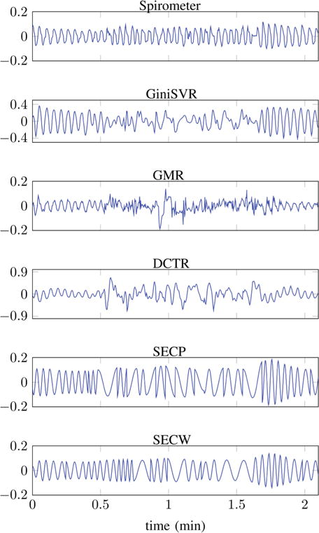
Test Signal-1: From top to bottom, plots of time series obtained from: Reference spirometer; GiniSVR (BR_err = 3.90 BPM, E_ρ = 0.4564); GMR (BR_err = 11.02 BPM, E_ρ = −0.0938); DCT based estimation (BR_err = 6.18 BPM, E_ρ = 0.0881); SECP (BR_err = 5.10 BPM, E_ρ = 0.8373) and SECW (BR_err = 3.90 BPM, E_ρ = 0.8126). Subject performing physical activity between 0.5 min to 1.5 min.

Fig. 12.

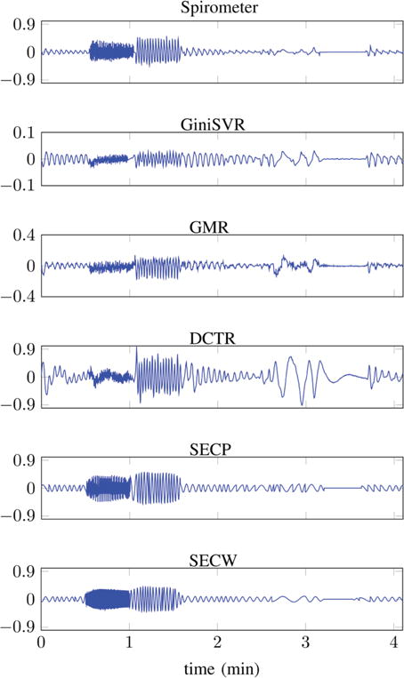
Test Signal-2: From top to bottom, plots of time series obtained from: Reference spirometer; GiniSVR (BR_err = 3.55 BPM, E_ρ = 0.3572); GMR (BR_err = 7.80 BPM, E_ρ = 0.8312); DCT based estimation (BR_err = 6.00 BPM, E_ρ = 0.3657); SECP (BR_err = 3.64 BPM, E_ρ = 0.9902) and SECW (BR_err = 2.54 BPM, E_ρ = 0.9885).

Fig. 12 displays the spirometer output and its estimates for a variety of respiratory states. The sequence of respiratory states is: normal breathing, tachypnea, hyperventilation, normal breathing, shallow breathing, slow deep-breathing, apnea and normal breathing. Test signal-2 does not contain any motion artifacts. Again it is apparent that the SEC based approaches result in the best estimate of the spirometer envelope. In terms of breathing rate, SECW gives the smallest error. In terms of envelope correlation coefficient, SECP is better (E_ρ = 0.99902) than SECW (E_ρ = 0.9885) but the difference is minimal. GiniSVR gives the best performance in terms of the breathing rate however, GMR is better than GiniSVR in terms of preserving the envelope information. GiniSVR employs only a single SVM and therefore, under-performs in accelerated breathing regions; notice, the attenuation of signal amplitude in tachypnea and hyperventilation regions. This is why employing multiple SVMs, in SECW, helps in obtaining a better estimate of the breathing rate.

Envelope and breathing rate estimation results averaged over 19 distinct human-subjects are shown in Figs. 13 and 14. Normal breathing sessions include sessions during which subject is breathing normally and performing different physical activities such as walking, reaching for object, rolling on bed etc. Accelerated breathing sessions also include apnea and slow breathing regions; in addition to tachypnea and hyperventillation; none of these sessions include motion artifacts. Results indicate that in accelerated breathing sessions, SECW results in the best envelope estimation performance E_ρ = 0.7411 ± 0.1434, this is followed by GMR and SEC at E_ρ = 0.6756 ± 0.2247 and 0.6734 ± 0.2207, respectively. GiniSVR results in E_ρ = 0.5912 ± 0.1537. In normal breathing sessions, GiniSVR gives the 2nd best performance E_ρ = 0.4691 ± 0.0962 after SECW E_ρ = 0.4717 ± 0.1040. In normal breathing sessions, E_ρ does not exceed 0.5 for any technique. This is because the envelope in normal breathing sessions is mostly flat (see for example test signal-1 in Fig. 11) and does not exhibit significant temporal variation. In these type of sessions a small spike or change in the envelope can cause significant decrease in value of the correlation coefficient. However, accelerated breathing sessions such as test signal-2 (12) exhibit significant temporal variation. In these sessions, a high correlation coefficient is very important. Results indicate that majority of the proposed algorithms seem to do a good job at tracking the temporal envelope in the accelerated breathing sessions.

Fig. 13.

Envelope correlation coefficient E_ρ for normal and accelerated breathing sessions; averaged over 19 different human subjects. Error bars indicate one standard-deviation.

Fig. 14.

Breathing rate error, BR_err, for normal and accelerated breathing sessions; averaged over 19 different human subjects. Error bars indicate one standard-deviation.

In terms of breathing rate estimation, Fig. 14 indicates that SECW gives the best performance in accelerated breathing sessions BR_err = 5.81 ± 3.34 (BPM). This is followed by GMR at BR_err = 7.48 ± 3.22 (BPM) and SECP at BR_err = 7.96 ± 6.60 (BPM). GiniSVR results in the highest BR_err in accelerated breathing sessions; this can be attributed to attenuation of high-frequency components in accelerated breathing sessions. However, in normal breathing sessions, GiniSVR is best performing approach with BR_err = 2.80 ± 0.63 (BPM). This indicates that of all the techniques discussed, GiniSVR is most robust to motion artifacts. Since, the carrier estimation of SECW is derived from GiniSVR it is also quite robust to motion artifacts and gives a BR_err = 3.09 ± 0.72 (BPM) which is slightly greater than that of GiniSVR. Overall, it seems that SECW benefits significantly from wavelet based regions identification and the use of adaptive GiniSVR for carrier estimation.

VI. Physical Activity Classification

A careful examination of the outputs of EIP channels during different physical activities indicates that each activity impacts the channel outputs in a distinct manner. For instance, differences in the EIP outputs during the three activities are quite prominent in Fig. 15. It can observed that coughing introduces high and low-frequencies. During reaching high-amplitude low-frequencies seem to be the dominant artifacts. A walk activity introduces distortions whose frequencies lie in between the (higher) frequency cough and the (lower) frequency reach distortions. This implies that we may be able differentiate between the underlying activity by examining the characteristics of channel outputs over time and frequency, provided that these characteristics do not vary significantly from one human-subject to another. The DWT score curves discussed in section IV-B1 are designed to capture the time-frequency signature of the EIP outputs. Therefore, these curves should also exhibit differences from one activity to another. If this is true then we should be able to classify the underlying physical activity by deriving simple features from the wavelet score curves. Results indicate that this is indeed the case.

Fig. 15.

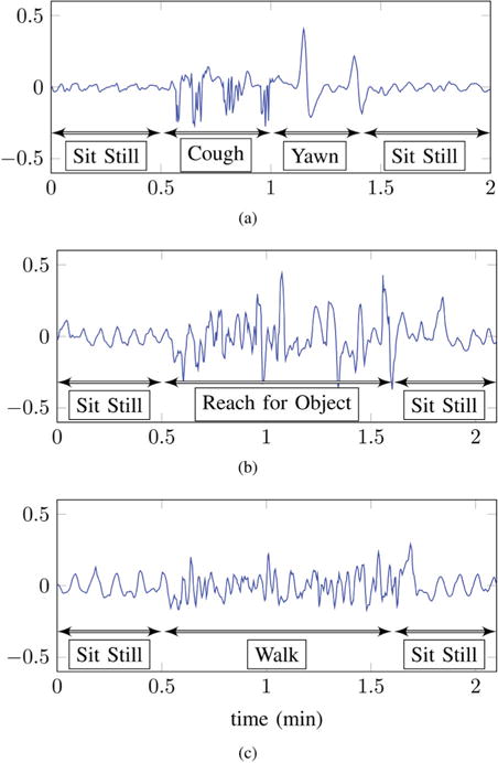
Output of an EIP channel during: (a) coughing (b) reaching and (c) walking activities.

A. Artifact Detection

The region score curves, employed for wavelet based respiratory state detection, provide a very simple but effective technique for artifact detection. A quick glance at the plots in Fig. 15 indicates that artifacts generally result in high amplitude jumps in the EIP outputs. The reference segment employed for evaluation of $\overline{p}[n]$ is artifact free therefore, the value of $\overline{p}[n]$ corresponding to artifact regions should be noticeably higher than 0.5. Examination of the wavelet score curves indicate that this is indeed the case. Therefore, an artifact region may be identified by examining the value of $\overline{p}[n]$. Values of $\overline{p}[n]$ greater than a threshold η(≫ 0.5) indicate the presence of an artifact. Whereas values of η ≤ 0.5 indicate artifact-free regions.

In order to gauge the accuracy of artifact detection achieved by thresholding the normal breathing score curve, $\overline{p}[n]$, we first divide each human-subject’s data into non-overlapping frames of 5 seconds each. Each frame is labeled based on whether it falls within an artifact or artifact-free region. During testing, error metrics are computed based on whether a frame is correctly classified. The true-positive rate (TPR) and false-positive rate (FPR) are then computed by decreasing the value of the threshold η from 1 to 0. At η = 1 the majority of the frames are classified as artifact-free, resulting low values of both TPR and FPR. Correct detection of artifact frames begin, as η is decreased from 1. A small number of false alarms are also generated however, the FPR is very low. The resulting ROC curve is shown in Fig. 16. This curve is calculated based on the data of all human-subjects. It can be observed that 90% of the frames in artifact regions can be classified correctly with a false-positive-rate of about 8%. A number of advantages are obtained by employing the wavelet based probabilistic score curve. The primary advantage is that the tradeoff between true-positives and false-alarms can be explicitly controlled by varying the threshold η. Additionally, the score-curves $\overline{p}[n]$ and p′[n] are exactly the same length as the input test signal and therefore provide good temporal resolution when identifying artifact regions.

Fig. 16.

ROC curve for artifact detection.

B. Artifact Classification

We present some features constructed from the score curves that allow differentiation between different physical activities. These features are then input to an SVM-classifier to classify different activities.

Feature Extraction

A human observer can classify most physical activities using just the score curves however, a pratical system needs to perform this task automatically with little (or no) human support. Such a systems requires a feature extraction frontend which can output, fixed-length, feature vectors that can be used by a learning algorithm to make accurate decision on its own. In this paper the task of the classifier is to make a decision about the physical activity performed in an input session. As mentioned in section II-A, each session is two minutes long on average and contains only one physical activity. For each session the wavelet score curves were computed according to the procedure outlined in section IV-B1. A number of different feature sets can be constructed from these curves. For a 2 minute long session the length of each raw score curve is 2 min × 40 samples/sec × 60 sec/min = 4800 samples long. Therefore, in their raw form the score curves are too high-dimensional to be employed as feature vectors. We investigate the following three distinct sets of feature vectors for classification of artifact sessions:

1. Curve-statistic features: These features are based on the statistics of the score curves and are listed in Table I. One of the potential shortcomings of the curve-statistic features is that they do not explicitly incorporate the temporal variations observed in the region score curves.

2. TF-signature features: In order to capture the temporal characteristics exhibited by $\overline{p}[n]$ and p′[n] in artifact sessions we construct another set of features which are obtained by simply downsampling the region score curves, by a constant rate, and reducing the length of each curve to N = 50 samples (extra samples at the end are truncated). Since the score curves vary slowly over time therefore, downsampling does not result in information loss and the shape of the curves is still retained. The downsampled curves are concatenated to form a 2N(= 100) dimensional feature vector. We refer to these features as (time-frequency) TF-signature features.

3. Sensor-curve features: For an input activity session these features are constructed by first taking mean of the output of the 10 EIP channels. This mean signal is then downsampled to a fixed length of 200 samples. Sensor-curve features may be considered to be a simplified form of TF-signature features; in the sense that they only incorporate the temporal and amplitude variations but do not attempt to capture the frequency variation by foregoing the wavelet transform used in the TF-signature features. The motivation for employing these features is to be able to gauge the performance-gain achieved by utilizing time-frequency signatures.

TABLE I.

Curve statistic features

Symbol	Interpretation
$\overline{\alpha }$	Maximum value of $\overline{p}[n]$ at artifact locations.
α′	Maximum value of p′[n] at artifact locations.
$\overline{\sigma }$	Standard deviation of $\overline{p}[n]$ at artifact locations.
σ′	Standard deviation of p′[n] at artifact locations.
$\overline{\mu }$	Mean value of $\overline{p}[n]$ at artifact locations.
μ′	Mean value of p′[n] at artifact locations.
μd	Mean value of $|p^{\prime }[n]-\overline{p}[n]|$ at artifact locations.

The extracted features are input to a support vector machine (SVM) classifier. Training and testing are performed on non-overlapping examples.

VII. Activity Classification Results

Our database contains a total of 129, two-minute long, sessions each containing a single physical activity. There are a total of 5 distinct physical activities (or classes) in the data. 31 of the sessions are recorded when the human-subjects are eating. 48 sessions are recorded with the subjects reaching to grab an object. In addition to these, there are 17 walk sessions, 16 cough sessions and 17 sessions recorded with the subjects rolling left-to-right on a bed. The classifier’s task is to determine the underlying physical activity in a given test session using the feature vector constructed from the electrode sensor outputs.

Since we do not have an extremely large number of sessions for training and testing therefore, we employ 4-fold cross-validation to evaluate the performance of the physical activity classification task. Data is split into 4 folds of approximately equal size; one fold is employed for testing while the remaining three folds are used for training. After, computation of error metrics for one fold it is swapped with another fold in the training data and the error metrics are recomputed. This procedure is repeated for all 4 folds and error metrics, averaged over all 4 folds and error metrics averaged over all 4 folds are computed. 4-fold cross-validation is repeated 30 times and the final average error metrics are computed. We employ two metrics to evaluate the performance of the classifier: (1) Accuracy and (2) Balance-Error-Rate or BER. The BER is employed since our class data is slightly unbalanced to larger instances of the eat and reach sessions. BER [33] is suitable for performance evaluation of unbalanced multi-class classification problems and is defined as:

$$\mathit{BER}=\frac{1}{M}{\displaystyle \sum _{i=1}^N\frac{\left({\displaystyle {\sum }_{j=1}^M{A}_{ij}}\right)-A_{ii}}{{\displaystyle {\sum }_{j=1}^N{A}_{ij}}}}$$ (25)

Here, A_ij denotes the element of the confusion matrix A located at the i^th row and the j^th column. It indicates the number of test vector of class-i that are predicted to belong to class-j. N and M represent the total number of test vectors and classes respectively.

Fig. 17 displays the average confusion matrices for curve-statistic and TF-signature features. The numbers in these plots indicate the average percentage of sessions, of each physical activity, that are classified correctly. For curve-statistic features, the reach activity has the highest detection rate (94%), followed by the roll activity (70%) and the eat activity (68%). The walk and cough activities have confusion rates, amongst each other and with the eat activity. The results obtained for sensor-curve features are presented only in terms of the accuracy and the BER metrics, the confusion matrix is not presented here due to space constraints. The average error metrics are presented in Table II; it can be observed that TF-signature features give the best performance both in terms of accuracy and BER. When compared to the simplistic sensor-curve features it the performance-gain, obtained from both curve-statistic and TF-signature features, is quite large. Both these features are derived from the wavelet-region-score curves; this indicates that the region-score curves do indeed capture the time-frequency behavior associated with different types of physical activities and thus provide us with an effective platform for activity classification.

Fig. 17.

Confusion matrix for: (a) Curve Statistics features and (b) TF-Signature features.

TABLE II.

Accuracy and BER for different feature types.

Feature Type	Accuracy	BER
Curve-Statistic	78.63%	25.97%
TF-signature	85.46%	15.11%
Sensor-Curve	46.62%	65.76%

VIII. Conclusions

We proposed a framework for virtual spirometry where multi-channel EIP is used in conjunction with bio-signal processing algorithms to robustly estimate the true spirometer output. We have experimented with a number of signal processing and filtering approaches using data collected from adult human-subjects. When the spirometer output is modeled by an amplitude-modulated signal, the results indicate that separate estimation of amplitude and breathing rate/carrier component outperforms joint estimation of both parameters. Detection of exact breathing rates in tachypnea or hyperventilation regions can be difficult however, wavelet filtering does seem to give reasonable performance but there is still room for improvement. We plan to investigate other approaches as part of our future work. In terms of motion artifacts, SVM-based regression, and other techniques derived from it, seem to give the best performance. We have also demonstrated that it is possible to classify physical activities based on the time-frequency signatures of the corresponding motion artifacts in the EIP channels. These features may be used separately or in conjunction with sensors such as accelerometers to provide improved physical activity monitoring.

Fig. 9.

Block diagram of wavelet based respiratory state detection.

Biographies

Hassan Aqeel Khan received his BSc degree in Electrical Engineering from the University of Engineering and Technology (UET), Taxila Pakistan in 2003 and his MSc degree in Signal Processing and Communication from the University of Edinburgh in 2007. And Ph.D. in Electrical and Computer Engineering from Michigan State University (MSU) in 2015. From 2004–2006 he was an Assistant Manager at the Pakistan Telecommunication Company Limited (PTCL). He is currently an Assistant Professor at the School of Electrical Engineering & Computer Science of the National University of Sciences and Technology (NUST) in Islamabad Pakistan. His research interests include biological & biomedical applications of signal processing and machine learning, wireless video coding, speech recognition and natural language processing.

Amit Gore received the Bachelors (B.E.) degree in Instrumentation Engineering from the University of Pune, India, in 1998, and the M.S. and Ph.D. degrees in Electrical Engineering from Michigan State University, East Lansing, in 2002 and 2008 respectively. He is currently working with GE Global Research, Niskayuna, NY as a Mixed Signal Designer. His research interests are multi-channel sigmadelta converters, charge to digital pipelined converters for low power biomedical devices, system design for CT products and life care solutions.

Jeffrey Ashe received the B.S. degree in electrical engineering from Clarkson University in 1989 and the M.S. degree in electrical engineering from Syracuse University in 1992. Mr. Ashe joined General Electric Aerospace in 1989 on the Edison Engineering Development Program and subsequently transferred to General Electric Corporate Research and Development in 1992. He is currently a Principal Engineer in bioelectronics at GE Global Research with interests in system engineering and signal processing for physiological monitoring. Jeff’s background includes radar, GPS, communication, instrumentation and electrical impedance tomography systems. Jeff has been a principal investigator for programs with the US Army, US Air Force, National Institute of Health and National Institute of Justice. He served as a federally appointed advisor to the US Department of Commerce Emerging Technologies and Research Advisory Committee (ETRAC) and is presently a visiting scientist in the Medical Electronics Device Realization Center (MEDRC) at Massachusetts Institute of Technology.

Shantanu Chakrabartty (SM’99-M’04-S’09) received his B.Tech degree from Indian Institute of Technology, Delhi in 1996, M.S and Ph.D in Electrical Engineering from Johns Hopkins University, Baltimore, MD in 2002 and 2004 respectively. He is currently a professor in the department of computer science and engineering at Washington University in St. Louis. From 2004–2015, he was an associate professor in the department of electrical and computer engineering at Michigan State University (MSU). From 1996–1999 he was with Qualcomm Incorporated, San Diego and during 2002 he was a visiting researcher at The University of Tokyo. Dr. Chakrabartty’s work covers different aspects of analog computing, in particular non-volatile circuits, and his current research interests include energy harvesting sensors and neuromorphic and hybrid circuits and systems. Dr. Chakrabartty was a Catalyst foundation fellow from 1999–2004 and is a recipient of National Science Foundation’s CAREER award, University Teacher-Scholar Award from MSU and the 2012 Technology of the Year Award from MSU Technologies. Dr. Chakrabartty is a senior member of the IEEE and is currently serving as the associate editor for IEEE Transactions of Biomedical Circuits and Systems, associate editor for the Advances in Artificial Neural Systems journal and a review editor for Frontiers of Neuromorphic Engineering journal.

References

- 1.Cretikos MA, Bellomo R, Hillman K, Chen J, Finfer S, Flabouris A. Respiratory rate: the neglected vital sign. Medical Journal of Australia. 2008;188(11):657. doi: 10.5694/j.1326-5377.2008.tb01825.x. [DOI] [PubMed] [Google Scholar]
- 2.Rodriguez-Roisin R. Toward a consensus definition for copd exacerbations. CHEST Journal. 2000;117(5 suppl 2):398S–401S. doi: 10.1378/chest.117.5_suppl_2.398s. [DOI] [PubMed] [Google Scholar]
- 3.Kristiansen NK, Fleischer J, Jensen M, Andersen KS, Nygaard H. Design and evaluation of a handheld impedance plethysmograph for measuring heart rate variability. Medical and Biological Engineering and Computing. 2005;43(4):516–521. doi: 10.1007/BF02344734. [DOI] [PubMed] [Google Scholar]
- 4.Luna-Lozano PS, García-Zetina OA, Pérez-López JA, Alvarado-Serrano C. Electrical Engineering, Computing Science and Automatic Control (CCE), 2014 11th International Conference on. IEEE; 2014. Portable device for heart rate monitoring based on impedance pletysmography; pp. 1–4. [Google Scholar]
- 5.Milanesi M, Martini N, Vanello N, Positano V, Santarelli M, Paradiso R, De Rossi D, Landini L. Engineering in Medicine and Biology Society, 2006 EMBS’06 28th Annual International Conference of the IEEE. IEEE; 2006. Multichannel techniques for motion artifacts removal from electrocardiographic signals; pp. 3391–3394. [DOI] [PubMed] [Google Scholar]
- 6.Milanesi M, Martini N, Vanello N, Positano V, Santarelli MF, Landini L. Independent component analysis applied to the removal of motion artifacts from electrocardiographic signals. Medical & biological engineering & computing. 2008;46(3):251–261. doi: 10.1007/s11517-007-0293-8. [DOI] [PubMed] [Google Scholar]
- 7.Griffiths A, Das A, Fernandes B, Gaydecki P. Journal of Physics: Conference Series. 1. Vol. 76. IOP Publishing; 2007. A portable system for acquiring and removing motion artefact from ecg signals; p. 012038. [Google Scholar]
- 8.Ansari S, Ward K, Najarian K. Epsilon-tube filtering: Reduction of high-amplitude motion artifacts from impedance plethysmography signal. IEEE journal of biomedical and health informatics. 2015;19(2):406–417. doi: 10.1109/JBHI.2014.2316287. [DOI] [PubMed] [Google Scholar]
- 9.Park S-B, Noh Y-S, Park S-J, Yoon H-R. An improved algorithm for respiration signal extraction from electrocardiogram measured by conductive textile electrodes using instantaneous frequency estimation. Medical & biological engineering & computing. 2008;46(2):147–158. doi: 10.1007/s11517-007-0302-y. [DOI] [PMC free article] [PubMed] [Google Scholar]
- 10.Shamim N, Atul M, Gari D C, et al. Data fusion for improved respiration rate estimation. EURASIP journal on advances in signal processing. 2010;2010 doi: 10.1155/2010/926305. [DOI] [PMC free article] [PubMed] [Google Scholar]
- 11.Orphanidou C, Fleming S, Shah S, Tarassenko L. Data fusion for estimating respiratory rate from a single-lead ecg. Biomedical Signal Processing and Control. 2013;8(1):98–105. [Google Scholar]
- 12.Dehkordi P, Tavakolian K, Marzencki M, Kaminska M, Kaminska B. Assessment of respiratory flow and efforts using upper-body acceleration. Medical & biological engineering & computing. 2014;52(8):653–661. doi: 10.1007/s11517-014-1168-4. [DOI] [PubMed] [Google Scholar]
- 13.Bao L, Intille SS. Activity recognition from user-annotated acceleration data. Pervasive computing Springer. 2004:1–17. [Google Scholar]
- 14.Chen KY, Acra SA, Majchrzak K, Donahue CL, Baker L, Clemens L, Sun M, Buchowski MS. Predicting energy expenditure of physical activity using hip-and wrist-worn accelerometers. Diabetes technology & therapeutics. 2003;5(6):1023–1033. doi: 10.1089/152091503322641088. [DOI] [PMC free article] [PubMed] [Google Scholar]
- 15.John D, Liu S, Sasaki J, Howe C, Staudenmayer J, Gao R, Freedson PS. Calibrating a novel multi-sensor physical activity measurement system. Physiological measurement. 2011;32(9):1473. doi: 10.1088/0967-3334/32/9/009. [DOI] [PMC free article] [PubMed] [Google Scholar]
- 16.Liu S, Gao RX, John D, Staudenmayer JW, Freedson PS. Multisensor data fusion for physical activity assessment. Biomedical Engineering, IEEE Transactions on. 2012;59(3):687–696. doi: 10.1109/TBME.2011.2178070. [DOI] [PubMed] [Google Scholar]
- 17.Lin C-W, Yang Y-TC, Wang J-S, Yang Y-C. A wearable sensor module with a neural-network-based activity classification algorithm for daily energy expenditure estimation. IEEE Transactions on Information Technology in Biomedicine. 2012;16(5):991–998. doi: 10.1109/TITB.2012.2206602. [DOI] [PubMed] [Google Scholar]
- 18.Scilingo EP, Lanata A, Tognetti A. Sensors for wearable systems. Wearable Monitoring Systems Springer. 2011:3–25. [Google Scholar]
- 19.Pacela AF. Impedance pneumographya survey of instrumentation techniques. Medical and biological engineering. 1966;4(1):1–15. doi: 10.1007/BF02474783. [DOI] [PubMed] [Google Scholar]
- 20.Oppenheim AV. Discrete-time signal processing. Pearson Education India; 1999. [Google Scholar]
- 21.Lathi BP. Modern Digital and Analog Communication Systems 3e Osece. Oxford university press; 1998. [Google Scholar]
- 22.Ashe JM, Ross AS. Separability of breathing from motion artifact using multi-lead electrical impedance pneumography measurements. Advanced Technology Applications for Combat Casualty Care (ATACCC) 2011 [Google Scholar]
- 23.Cortes C, Vapnik V. Support-vector networks. Machine learning. 1995;20(3):273–297. [Google Scholar]
- 24.Guyon I, Boser B, Vapnik V. Automatic capacity tuning of very large vc-dimension classifiers. Advances in neural information processing systems. 1993:147–147. [Google Scholar]
- 25.Chakrabartty S, Cauwenberghs G. Gini support vector machine: Quadratic entropy based robust multi-class probability regression. The Journal of Machine Learning Research. 2007;8:813–839. [Google Scholar]
- 26.Gauvain J-L, Lee C-H. Maximum a posteriori estimation for multivariate gaussian mixture observations of markov chains. Speech and audio processing, ieee transactions on. 1994;2(2):291–298. [Google Scholar]
- 27.Reynolds DA, Quatieri TF, Dunn RB. Speaker verification using adapted gaussian mixture models. Digital signal processing. 2000;10(1):19–41. [Google Scholar]
- 28.Bishop CM, Nasrabadi NM. Pattern recognition and machine learning. Vol. 1 springer; New York: 2006. [Google Scholar]
- 29.Lloyd S. Least squares quantization in pcm. Information Theory, IEEE Transactions on. 1982;28(2):129–137. [Google Scholar]
- 30.Dempster AP, Laird NM, Rubin DB, et al. Maximum likelihood from incomplete data via the em algorithm. Journal of the Royal statistical Society. 1977;39(1):1–38. [Google Scholar]
- 31.Daubechies I, et al. Ten lectures on wavelets. Vol. 61 SIAM; 1992. [Google Scholar]
- 32.Mallat SG. A theory for multiresolution signal decomposition: the wavelet representation. Pattern Analysis and Machine Intelligence, IEEE Transactions on. 1989;11(7):674–693. [Google Scholar]
- 33.Read I, Cox S. Automatic pitch accent prediction for text-to-speech synthesis [Google Scholar]