Volumetric image registration from invariant keypoints

Abstract

We present a method for image registration based on 3D scale- and rotation-invariant keypoints. The method extends the Scale Invariant Feature Transform (SIFT) to arbitrary dimensions by making key modifications to orientation assignment and gradient histograms. Rotation invariance is proven mathematically. Additional modifications are made to extrema detection and keypoint matching based on the demands of image registration. Our experiments suggest that the choice of neighborhood in discrete extrema detection has a strong impact on image registration accuracy. In head MR images, the brain is registered to a labeled atlas with an average Dice coefficient of 92%, outperforming registration from mutual information as well as an existing 3D SIFT implementation. In abdominal CT images, the spine is registered with an average error of 4.82 mm. Furthermore, keypoints are matched with high precision in simulated head MR images exhibiting lesions from multiple sclerosis. These results were achieved using only affine transforms, and with no change in parameters across a wide variety of medical images. This work is freely available as a cross-platform software library.

I. Introduction

Medical image registration is the task of aligning a pair of medical images by mapping relevant objects to the same coordinates. It is an essential preprocessing step in a wide variety of imaging tasks, especially those involving morphology and localization of lesions, brain activity, or other objects of interest. While most work has focused on intensity-based registration, in which all image data is considered, there has been some interest in addressing the problem via local keypoints [1]–[5]. Keypoints are stable image coordinates selected by purely local or shift-invariant operations, and matched between images based on local information. Unlike intensity-based methods, keypoint-based methods do not require initialization and cannot converge to local minima. Furthermore, they succeed despite anatomical differences which would otherwise necessitate preprocessing. For example, tissue containing lesions can be registered based on information local to normal anatomy. Similarly, scans showing different organs, such as the abdomen and full body, can be registered without the need to remove inconsistent anatomy.

Many methods have been proposed for detecting and describing keypoints in two-dimensional images [6]–[8]. However, less attention has been paid to three-dimensional or volumetric images. Our past work and the work of others has shown that unique challenges arise in higher dimensions, necessitating modifications to the usual keypoint algorithms [2], [5], [9], [10]. In particular, orientation assignment and the geometry of gradient histograms are more complicated in ℝⁿ, as ℝ² is revealed to be a special case.

This work offers three main contributions. First, we present a generalization of the Scale-Invariant Feature Transform (SIFT) algorithm to ℝⁿ, with particular attention paid to ℝ³. The generalized algorithm differs mainly in orientation assignment and gradient histogram geometry. These modifications allow the resulting keypoints to achieve the same invariances to scale and rotation in ℝⁿ as the original has in ℝ². In particular, rotation invariance is mathematically proven in ℝⁿ. Secondly, we present a new analysis of the choice of neighborhood in discrete extrema detection, which is necessary for accurate results in our experiments. Finally, we develop a fully-automatic image registration system based on keypoint matching that succeeds on a wide variety of medical images.

In our experiments, keypoint-based methods outperform registration from mutual information, and the proposed method outperforms an exiting approach to 3D SIFT. Using only affine transforms, the proposed method aligns the brain to an atlas in head magnetic resonance (MR) images with an average Dice coefficient of 92%, and registers the spine in longitudinal computed tomography (CT) studies with an average error of 4.82 mm. Keypoints are matched with high precision in simulated head MR images exhibiting multiple sclerosis (MS) lesions, despite arbitrary rotations. The same parameters succeed on this wide range of medical images. To enable adoption into more complex systems, this work is freely available as a cross-platform software library [11].

II. Related work

There have been several previous efforts to extend SIFT keypoints to higher dimensions. The first application was for video action recognition [10]. Soon after, various authors explored SIFT feature matching for various applications in volumetric imaging. Ni et al. applied 3D SIFT to ultrasound panorama construction, while Flitton et al. experimented with recognition of non-medical objects [3], [12]. Cheung and Harmeneh developed an n-dimensional extension of SIFT and experimented with matching keypoints in various MR and CT images [1]. While these works showed encouraging results for various applications, the approaches used were theoretically flawed, as the method of orientation estimation did not account for true 3D rotations, and the histogram geometry made the descriptors anisotropic.

Corrections to some of these problems have appeared previously in the literature. Kldser et al. corrected the problem of histogram geometry, but to our knowledge this work on video processing was not adopted in the literature on medical image analysis [9]. Allaire et al. developed a method for estimating 3D orientation by extending the gradient histogram approach of the original SIFT [2]. The same method of orientation invariance was adopted by Toews et al., among other innovations, and evaluated on abdominal CT and head MR registration [4]. However, all of these approaches suffer from quantization due to histogram bins, and to our knowledge none of them has simultaneously provided a correct method for both orientation estimation and histogram geometry in three dimensions. In this work we propose an extension of SIFT to 3D which addresses these theoretical difficulties. We propose a method of orientation estimation based on eigendecomposition of the structure tensor, which we prove accounts for arbitrary rotations in any number of dimensions. Furthermore, we base our gradient histograms on the regular icosahedron, interpolating contributions between histogram bins by the barycentric coordinates of the triangular faces, which mitigates quantization effects in a geometrically plausible way. To our knowledge, these approaches have not been previously used for 3D keypoints, and resolve the mathematical issues of previous work.

In addition to theoretical contributions, this work contains several practical innovations. First, we examine the role of neighborhood choice in discrete extrema detection, demonstrating experimentally that the ℓ¹ neighborhood outperforms the ℓ^∞ neighborhood for medical image registration. Second, we explore the use of 3D SIFT keypoints with a different feature descriptor based on geometric moment invariants (GMIs), comparing the performance between the SIFT and GMI descriptors. Finally, we offer an open-source, cross-platform implementation, usable in both C and Matlab, which was lacking in the existing literature [11].

III. Keypoint detection and description

There are two stages to extracting keypoints from an image. The first involves detecting points which can be reliably matched between pairs of images. The second involves generating a feature vector describing the image content in a window centered at each point. The resulting feature vectors, called “descriptors,” are approximately invariant to dilation, rotation, and translation of the underlying image. The following section summarizes these methods, proceeding by analogy to the SIFT algorithm, which was originally defined for two-dimensional images.

A. Keypoint locations

Candidate keypoint locations are obtained in much the same way as in the original SIFT algorithm [6]. To approximate scale invariance, we search for maxima of both the image space coordinate x, and a Gaussian scaling parameter, σ. The vector (x, σ) is called a “scale-space” coordinate. The function to be maximized is the image convolved with the Laplacian of Gaussian function

$$\ell (\mathbf{x},\sigma )=I(\mathbf{x})\ast \mathrm{\Delta }{g}_{\sigma }(\mathbf{x}),$$ (1)

where g_σ(x) is a Gaussian function of parameter σ [13]. This is approximated by convolution with the difference of Gaussians (DoG) function

$$d(\mathbf{x},\sigma )=I(\mathbf{x})\ast (g_{\sigma +\delta }(\mathbf{x})-g_{\sigma }(\mathbf{x})),$$ (2)

where δ is a small constant [6]. The DoG function is computed by subtracting successive levels of a Gaussian scale-space pyramid.

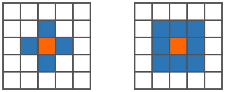
The extrema of d(x, σ) form the initial keypoint candidates. While past authors have usually defined extrema as maxima and minima of the (3ⁿ – 1)-connected ℓ^∞ neighborhood, we define extrema using the 2n-connected ℓ¹ neighborhood, as seen in figure 1. These neighborhoods are known in cellular automata theory as the Moore and von Neumann neighborhoods, respectively. The ℓ¹ extrema are a superset of those found with the ℓ^∞ neighborhood. Defining extrema in this way lends itself to the theoretical interpretation that a point is an ℓ¹ extremum only if it is a stationary point of its forward differences¹. While this results in a considerable increase in the number of extrema, and thus the necessary computation, it yields a far greater number of correctly matched keypoints².

Fig. 1.

Visualization of the ℓ¹ (left) and ℓ^∞ (right) neighborhoods in ℤ². In our experiments, defining extrema with the ℓ¹ neighborhood improves registration results.

Having found our initial candidates, we reject those weak in magnitude. Formally, we reject a candidate (x, σ) if

$$|d(\mathit{x},\sigma )|<\alpha \underset{\mathbf{x},\sigma }{max}|d(\mathbf{x},\sigma )|,$$ (3)

where α is a constant parameter. This differs slightly from the original SIFT formulation, as the max term in equation 3 adapts the threshold to the contrast of our data [6]. Unlike the original SIFT, we do not interpolate keypoint coordinates to sub-voxel accuracy, as this failed to improve matching stability in our experiments [14].

B. Local orientations and corner detection

In order to construct rotation-invariant feature descriptors, it is common practice to assign a repeatable orientation to each keypoint [6]–[8]. By rotating the windowed image according to the inverse of its orientation, the feature descriptor is made invariant to rotations of its object. Information related to the orientation is also used to reject poorly-localized objects, such as plate- and tube-like structures in ℝ³.

Keypoint detection algorithms in ℝ² typically assign to each keypoint an angle θ, from which a rotation matrix is computed. In SIFT, θ is selected according to a mode of a gradient histogram computed in a window around the keypoint. In truth ℝ² is a special case, and this approach does not generalize to higher dimensions [2]. A rotation matrix in ℝⁿ is an orthogonal matrix R ∈ ℝ^n×n with |R| = 1. Analogous to the two-dimensional case, such a matrix may be formed by trigonometric functions of n Euler angles. But, (n – 1)-spherical coordinates yield only n – 1 angles. Thus, we cannot define an orientation by selecting only one vector from the gradient histogram. Nevertheless, Scovanner et al. used the two Euler angles given by spherical coordinates to produce a rotation matrix in ℝ³, admitting that this approach does not cover the general case [10]. Accordingly, much of the prior work on 3D SIFT was not rotation-invariant [1], [3], [9], [10], [12], [15].

Allaire et al. circumvented this issue by first selecting a vector from the gradient histogram, and then computing an additional histogram in its plane through the origin [2], [4]. In ℝ³, finding the mode of this secondary histogram amounts to computing the “roll” about the first vector. Besides the computational cost, a problem for this approach is quantization by the histogram bin angles. A simple alternative for orientation assignment, isotropic and applying to any number of dimensions, is to utilize the correlation between gradient components, also known as the structure tensor,

$$K=\int w(\mathbf{x})\nabla I(\mathbf{x}){(\nabla I(\mathbf{x}))}^{T}d\mathbf{x}$$ (4)

where ∇I(x) is the gradient of image I at location x, approximated by finite differences, and w(x) is a Gaussian window centered at the keypoint, the width of which is a constant multiple of the keypoint scale.

The structure tensor is real and symmetric, and thus it has an orthogonal eigendecomposition, K = QΛQ^T. If the eigenvalues are ordered and distinct, then the decomposition is unique except for negation of columns of Q. A graphical interpretation of the structure tensor and its eigenvectors is given in figure 2. This matrix is well-known in computer vision, especially with regard to corner detection. Kandel et al. used these eigenvectors to align pairs of image patches [16]. In this work, we use them to derive an orientation local to each keypoint, obviating the need for pairwise alignment.

Fig. 2.

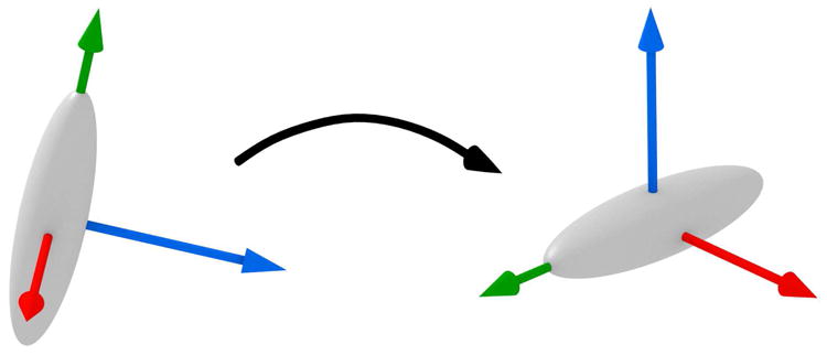
The structure tensor, represented as an ellipsoid, under rotation. The chosen eigenvectors undergo the same rotation.

The matrix Q cannot give a robust orientation per se, as it is ambiguous as to the direction of change along each axis. To see this, consider that Q is invariant to negation of ∇I. We must incorporate more information to achieve rotation invariance. A natural choice is to compute the direction of change along each vector q_i, the i^th column of Q, which is just the sign of the directional derivative

$$\begin{array}{c}\mathit{d}=\int w(\mathbf{x})\nabla I(\mathbf{x})\mathit{d}\mathbf{x}\\ s_i=sgn({\mathit{q}}_i^T\mathit{d})\end{array}$$ (5)

We remove this ambiguity by requiring that the directional derivative of each eigenvector is positive, computing the columns of R as r_i = s_iq_i. Here we reject keypoints with s_i = 0 as degenerate. Then, s_i ∈ {−1, 1}, so $s_k^2=1$. Expanding terms we have

$${(R\mathrm{\Lambda }{R}^T)}_{ij}=\sum _{k=1}^n{\lambda }_k(s_k{Q}_{ik})(s_k{Q}_{jk})$$ (6)

so that K = RΛR^T. Intuitively, this states that negation of any eigenvectors still yields an eigendecomposition of K. This fact allows us to prove that the matrix R tracks rotation of the image data about the keypoint³. It also allows us to avoid reflections, having |R| = −1, by negation of r_n. The structure tensor is not unique in having these properties, for example a rotation matrix can be recovered by a similar process of eigendecomposition and sign correction using third-order image moments [17]. Compared to that approach, we prefer the structure tensor due to its simplicity and computational expedience.

In the previous discussion we have assumed that the eigenvectors and their directional derivatives were reliably computed. In practice, this holds only for certain data. We now introduce criteria to reject degenerate keypoints, which would not be reliably oriented. We first verify the stability of the eigenvectors, rejecting a keypoint if ${max}_i|\frac{{\lambda }_i}{{\lambda }_{i+1}}|>\beta$, where λ_i is the i^th eigenvalue of K, in ascending order, and β a constant parameter. Next, we test the angle between the gradient d and eigenvectors q_i,

$$cos({\theta }_i)=\frac{{\mathit{q}}_i^T\mathit{d}}{\Vert {\mathit{q}}_i\Vert \Vert \mathit{d}\Vert }.$$ (7)

The directional derivative is unstable when the two vectors are nearly perpendicular. Thus, we reject a keypoint if min_i |cos(θ_i)| < γ, a constant parameter. This also serves as a method of corner detection, rejecting points at which the image is nearly invariant in the direction of q_i. For example, in ℝ³ a tube-like structure is nearly invariant along a single axis, while a plate-like structure is poorly-localized in a plane. We omit testing the ratio |λ_n/λ₁| which was approximated by many corner detectors, including the original SIFT, as in our experiments it gives similar results to the proposed angle test [6], [18]. These two criteria remove a large fraction of the unreliable keypoints.

C. Gradient histograms

Gradient histograms are a robust representation of local image data [6], [19]. A gradient histogram estimates the distribution of image gradients in a window, with bins assigned based on the direction of the gradient vector ∇I(x), and contributions weighted by the magnitude |∇I(x)|. In SIFT, the polar angle is divided evenly into eight bins, with each bin sweeping $\frac{\pi }{4}$ radians [6]. Here again, ℝ² is a special case, as we cannot divide the possible directions in ℝⁿ into bins in such a simple way. Previous authors extended this concept to higher dimensions by converting the gradient to (n – 1)-spherical coordinates, dividing each angle into bins of the same increment [1]–[4], [10], [12], [15]. We refer to this as the “globe” method, because the edges between bins are the same as the lines of longitude and latitude in a globe. As noted by Scovanner et al., this histogram is biased towards certain directions in ℝ³ [10]. The problem can be seen by viewing the gradient histogram as a tessellation of the unit (n – 1)-sphere. Here, a gradient vector is assigned to the bin intersected by the ray sharing its direction and origin. As shown in figure 3, the globe results in differently-shaped tiles.

Fig. 3.

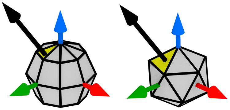
Left: histogram bins by evenly-spaced spherical coordinates. Right: Icosahedral histograms. The yellow tile is intersected by the gradient vector, shown in black.

Viewing the problem in this way, it is clear that we must tessellate the (n – 1)-sphere into congruent tiles, with each vertex incident to the same number of tiles. The number of convex polytopes satisfying these constraints depends on n [20]. In three dimensions, they are given by the five Platonic solids. Of these, we choose the regular icosahedron, having the largest number of faces. Similar methods based on Platonic solids were previously developed for human action recognition in video sequences of two-dimensional images [9], [21].

Although the histogram is now evenly weighted between tiles, it is still subject to artifacts due to quantization of the gradient directions. To mitigate this effect, we change the histogram again, so that the bins are the vertices of the icosahedron, rather than its faces. To accumulate a gradient vector into a bin, we interpolate its magnitude between the three vertices incident to its intersecting triangle, as shown in figure 4. This is equivalent to interpolating onto the three nearest face centers of the dual graph, the regular dodecahedron. We use as interpolation weights the barycentric coordinates of the point where the gradient ray intersects the triangle. This is computationally efficient, as the barycentric coordinates are already computed to test for ray-triangle intersection via the Mvller-Trumbore algorithm [22].

Fig. 4.

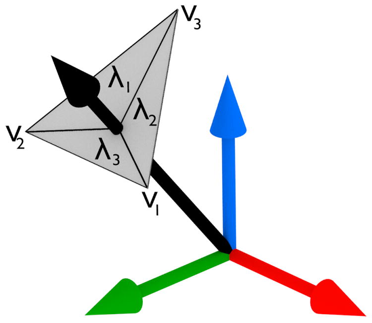
A vector is interpolated onto the vertices of its intersecting triangle, where λ_i is the interpolation weight at ν_i.

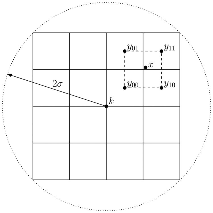
To compute the keypoint descriptor, also known as the feature vector, we first take a spherical image window centered at the keypoint, of radius 2σ, where σ is a constant multiple of the keypoint scale from equation 2. To achieve rotation invariance, the image is rotated by the inverse of the keypoint orientation from section III-B. The spherical window is then divided into a 4 × 4 × 4 array of cubical sub-regions, as seen in figure 5. A separate gradient histogram is computed for each sub-region, with 12 vertices per histogram, giving 4³ · 12 = 768 components in total. Using a Gaussian window, the contribution of each voxel is weighted by a Gaussian function of scale σ, based on its distance to the keypoint. To avoid quantization, the contribution of each voxel is distributed by barycentric coordinates between the three vertices of its intersecting triangle, and by trilinear interpolation between the eight sub-region centers enclosing the voxel in a cube. Thus, if the keypoint location is k, the sub-region is centered at y, and (λ₁, λ₂, λ₃) are the barycentric coordinates of the point where the gradient ray intersects the face of the icosahedron, the value added by voxel x to the bin corresponding to λ_i is

Fig. 5.

Visualization of trilinear interpolation from equation 8 in two dimensions. The coordinate system is centered and rotated around the keypoint k. The descriptor is computed in a window of radius 2σ. The gradient magnitude at x is weighted according to its distance from the subregion centers y_ij, which enclose x in a square. In three dimensions, there are eight subregions y_ijk enclosing x in a cube.

$${\lambda }_i\Vert \nabla I(\mathbf{x})\Vert exp(-\frac{{\Vert \mathbf{x}-k\Vert }^2}{2{\sigma }^2})\prod _{i=1}^n(1-\frac{\sigma }{\sqrt{2}}|{\mathbf{x}}_i-y_i|)$$ (8)

where the exponential term is the Gaussian window, and the product term is the trilinear interpolation weight for y. This is analogous to the original SIFT formulation, but it interpolates over triangles instead of circular arcs, and cubes instead of squares [6]. After all values have been accumulated, the descriptor is ℓ² normalized, truncated by a constant threshold δ, and normalized again [6].

D. Geometric moment invariants

Although the original SIFT descriptor was based on gradient histograms, it is possible to interchange keypoint detectors and descriptors. For comparison, we implemented a different feature descriptor based on geometric moment invariants. In this context, moments are functions mapping images to real numbers, having the form

$$M_{pqr}(I)\int \int {\int }_{\Vert (x,y,z)\Vert <R}{x}^p{y}^q{z}^{r}I(x,y,z)dxdydz$$ (9)

where p, q, r ∈ ℕ, I : ℝ³ → [−1, 1] is the image and R > 0 is the window radius. GMIs are polynomials of these moments, which have been shown to be invariant to various geometric transformations. These quantities were used as feature vectors to match anatomical locations in the HAMMER registration algorithm [23]. In this work, we form a feature vector from the second-order rotation-invariant polynomials

$$\begin{array}{c}{J}_0=M_{000}\\ J_1=M_{200}+M_{020}+M_{002}\\ J_2=M_{200}{M}_{020}+M_{200}{M}_{002}+M_{020}{M}_{002}-M_{101}^2-M_{110}^2-M_{011}^2\\ J_3=M_{200}{M}_{020}{M}_{002}+2M_{110}{M}_{101}{M}_{001}-M_{002}{M}_{110}^2-M_{020}{M}_{101}^2-M_{200}{M}_{001}^2\end{array}$$ (10)

which were studied by several authors [17]. The first GMI is proportional to the mean intensity, while the others are more difficult to interpret. Since these quantities will be vastly different in magnitude, we first define the normalizing constant

$$\Vert M_{pqr}\Vert =\int \int {\int }_{\Vert (x,y,z)\Vert <R}|x^p{y}^q{z}^r|dxdydz$$ (11)

which is just the moment of the function I(x, y, z) = sgn(x^py^qz^r), the largest possible value of M_pqr. Then we compute the normalized GMIs

$$\begin{array}{c}{\stackrel{\sim }{J}}_0=\frac{J_0}{\Vert M_{000}\Vert }\\ {\stackrel{\sim }{J}}_1=\frac{J_1}{\Vert M_{200}\Vert +\Vert M_{020}\Vert +\Vert M_{002}\Vert }\\ \dots \end{array}$$ (12)

These constants suffice to map each GMI to roughly the same range. However, we still have the issue that J₂ and J₃ are second- and third-order polynomials, making them more sensitive to changes in the moments than J₁ or J₂. To compensate for this, we use the final mapping

$$\begin{array}{c}{\overline{J}}_2={\stackrel{\sim }{J}}_2/\sqrt{|{\stackrel{\sim }{J}}_2|}\\ {\overline{J}}_3={\stackrel{\sim }{J}}_3/{|{\stackrel{\sim }{J}}_3|}^{2/3}\end{array}$$ (13)

with J̄₀ = J̃₀ and J̄₁ = J̃₁. It is clear that the normalized GMIs have the same geometric invariances as the originals. As in the original HAMMER work, we found that discriminative matching requires taking GMIs centered at multiple voxels in a neighborhood around the keypoint, although this destroys rotation invariance. We took R = 11 and concatenated GMIs from a 5 × 5 × 5 image window centered at the keypoint, yielding a descriptor with 5³ · 4 = 500 components. These parameters were chosen to yield a computation time and feature vector size comparable to our 3D SIFT descriptor.

IV. Keypoint matching and image registration

We now review how to register a pair of images from keypoints. This consists of two phases, matching the keypoints to establish corresponding locations, and fitting a transformation to the correspondences.

A. Keypoint matching

In keypoint matching, we identify a subset of the keypoints in one image appearing in the other. More formally, given a set S₁ of keypoint descriptors in the source image, and S₂ in the reference image, we wish to find a bijection from some subset S̃₁ ⊂ S₁ to another S̃₂ ⊂ S₂. We allow subsets because some keypoints may not be present in the other image, due either to occlusion, field of view, or failure in keypoint detection. Given a metric d(x, y) over feature descriptors, we can order the members of S₂ by their distance to a descriptor in S₁. We use the Euclidean distance for d, as it is inexpensive to compute and gives the best results of the metrics we tried. Let x ∈ S₁, and let y_i ∈ S₂ be the i^th-nearest member of S₂ to x. Lowe defined the matching score

$$g(\mathbf{x},S_2)=\frac{d(\mathbf{x},{\mathbf{y}}_1)}{d(\mathbf{x},{\mathbf{y}}_2)}$$ (14)

which is small when the match between x and y₁ is particularly distinctive, i.e. x is much closer to y₁ than to any other member of S₂ [6]. Thus, we say that x matches y₁ if g(x, S₂) is below some threshold η. This prevents matching when keypoints are locally similar, which often occurs in medical images.

The previous criterion is neither symmetric nor injective. That is, the matches from S₁ to S₂ need not be the same as those from S₂ to S₁. To address this limitation, we perform the procedure in each direction, S₁ → S₂ and S₂ → S₁, rejecting matches for which the two passes disagree. Note that we need only compute g(y, S₁) for each y ∈ S₂. In practice |S̃₂| is often a small fraction of |S₂|, so the bijective matching algorithm is only slightly more expensive than the original.

B. Image registration

Having extracted keypoints and matched them in a pair of images, we register the images by fitting a geometric transformation to these correspondences. In this work we will only use affine transforms, which are simple mathematically and suffice to register our data. Given a coordinate x ∈ ℝⁿ, with parameters A ∈ ℝ^n×n and b ∈ ℝⁿ, an affine transform has the form x′ = Ax + b. This characterizes all translations, dilations, rotations and reflections, among other operations. It is a linear operator in ℝⁿ⁺¹, as we have

Algorithm 1 Fitting a function via RANSAC

Let f : ℝn → ℝn be the function we wish to fit. Furthermore, let $S={\{({\mathbf{x}}_k,{\mathbf{y}}_k)\}}_{k=1}^m$, such that xk ∈ ℝn corresponds to yk ∈ ℝn. N and ε are parameters.

I* ← ø

for i = 1, …, N do

Fit f to a randomly drawn subset of S

I ← {(x, y) ∈ S : ‖f(x) – y‖ < ε}

if |I| > |I*| then

I* ← I

end if

end for

Fit f to I*

$$\left(\begin{array}{c}{\mathbf{x}}^{\prime }\\ 1\end{array}\right)=\left(\begin{array}{cc}A& \mathbf{b}\\ 0^T& 1\end{array}\right)\left(\begin{array}{c}\mathbf{x}\\ 1\end{array}\right).$$ (15)

As such we can fit an affine transform by linear regression, requiring at least n + 1 matches for uniqueness. Some of the matches will be erroneous, so we reject outliers by Random Sample Consensus (RANSAC) as in algorithm 1 [24]. This attempts to find the transform with the most inliers, by iteratively fitting transforms to subsets of the data. The final transformation is the least squares fit to the inliers, where the error is the Euclidean distance in millimeters.

V. Experiments

In this section, we present experiments showing the robustness of keypoint-based image registration, and the necessity of the proposed modifications to the original SIFT algorithm. We test on three types of data, each demonstrating a different image registration task, where we compute a different kind of accuracy. The first test is intra-patient registration of simulated multiple sclerosis (MS) cases, in which we compare different variations on 3D SIFT detectors and descriptors. The second test is inter-patient registration of simulated normal brain MRIs, in which we compare our feature-based method to intensity-based image registration. The final test is intra-patient registration of real abdominal CT scans from longitudinal cancer studies, in which we evaluate the accuracy of the algorithm on a challenging real-world use case.

We used the same parameters for all tests, to avoid over-fitting to the test data. The keypoint parameters from section III were α = 0.1, β = 0.9, γ = 0.5 and δ = 0.0335. The Gaussian scale-space pyramid from section III-A assumed an initial scale of σ_n = 1.15, a base scale of σ₀ = 1.6, and six levels per octave. We refer the readers to the original SIFT literature for the meaning of these parameters [6]. Except in figure 7, the matching threshold from section IV-A was η = 0.8. Finally, algorithm 1 used N = 2500 iterations and ε = 20 mm, except for the MS experiment in section V-A where ε was the same as the error threshold. Most of the code was implemented in ANSI C, with OpenMP multithreading. All experiments were run on all four cores of an Intel Core i5-4590 CPU. Although the processing time and accuracy depend heavily on the parameters, these values suffice for a wide range of medical imaging tasks.

Fig. 7.

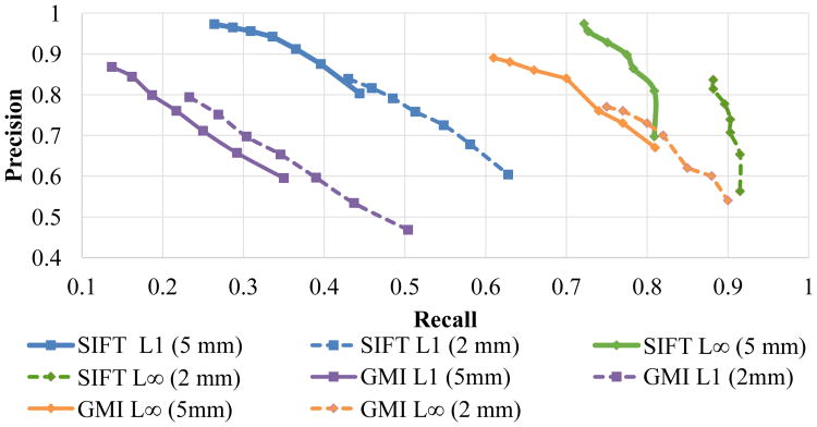
Precision-recall curves for the MS experiment, obtained by varying η in the interval [0.7, 1.0], for two different values of ε.

A. Brain MR with MS lesions

The following experiment simulates registration of brain MRIs from an MS patient over time. The reference image is of a normal brain, and the source or moving image is of the same brain, but with severe lesions. The test images come from the BrainWeb MRI simulator, using T2 weighting, 1 mm resolution, 3% noise, and 20% field nonuniformity [25]. To simulate clinical conditions, we rotated the source image by 10° about the z axis. Figure 6 shows a slice of the test images, along with matches from the proposed method. Because the data come from the same anatomical model, we have the ground truth displacement at each voxel, so we can verify each matched keypoint independently. This allows us to compute precision and recall for different versions of 3D SIFT features.

Fig. 6.

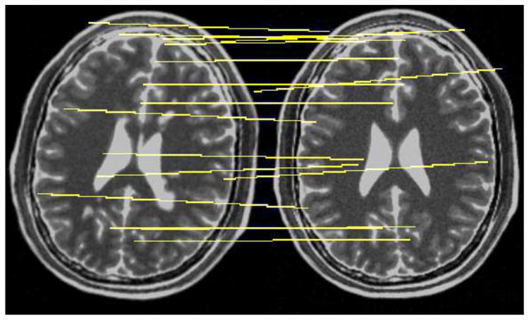
The rotated head with MS lesions (left) and normal head (right), with matches in this slice drawn in yellow.

The evaluation methodology is as follows: a true correspondence is one within ε mm of the ground truth, and a positive is a matched keypoint in the source image. For example, a false positive is a keypoint which was assigned an incorrect match, while a false negative is a keypoint for which a true correspondence exists in the other image, but was not assigned a match. From these definitions, we computed the standard precision and recall scores,

$$\begin{array}{c}\text{precision}=\frac{\text{true positive}}{\text{true positive}+\text{false positive}}\\ \text{recall}=\frac{\text{true positive}}{\text{true positive}+\text{false positive}}.\end{array}$$

We also computed the mean squared error (MSE) of the resulting affine transformation, taken as the squared distance between the matched keypoint and the ground truth location in the reference image, averaged over each keypoint in the source image.

We tested two versions of 3D SIFT features, one with the ℓ¹- and one with the ℓ∞-neighborhood, as described in section III-A. We also tested the GMI features from section III-D with each of the two neighborhoods. To reduce the dependence of the experiment on the error threshold, we computed the scores for ε = 2 and ε = 5, which are reasonable thresholds for many problems in medical image analysis. Despite the theoretical differences, in our experiments the global and icosahedral histograms of section 3 yielded equivalent results. Thus we chose the icosahedron, as it is theoretically superior and results in a smaller feature descriptor.

In this experiment the ℓ^∞ neighborhood yielded higher recall, but fewer total matches, as shown in figure 7 and table I. This is intuitive, as we would expect a more conservative choice of keypoints to reduce the chance of error. Nevertheless, for this application it is indispensable that we have a sufficient number of matches, and we shall see in: section V-B that the ℓ¹ neighborhood is essential for accurate inter-patient registration. For each choice of neighborhood, the SIFT descriptor yielded more matches, and higher precision and recall, and lower MSE than the GMI descriptor. This suggests it is a more distinctive representation of the underlying image than the GMI descriptor.

Table I.

Keypoint matches, registration error and execution times for the MS experiment.

Neighborhood	ℓ∞		ℓ1
Keypoints	487		10370
Descriptor	SIFT	GMI	SIFT	GMI
True matches, ε = 2 mm	129	113	2229	1385
True matches, ε = 5 mm	154	133	2695	1587
Total matches	166	155	2818	1986
Mean squared error (mm)	.43	.69	.47	.58
Execution time (s)	61	74	201	190

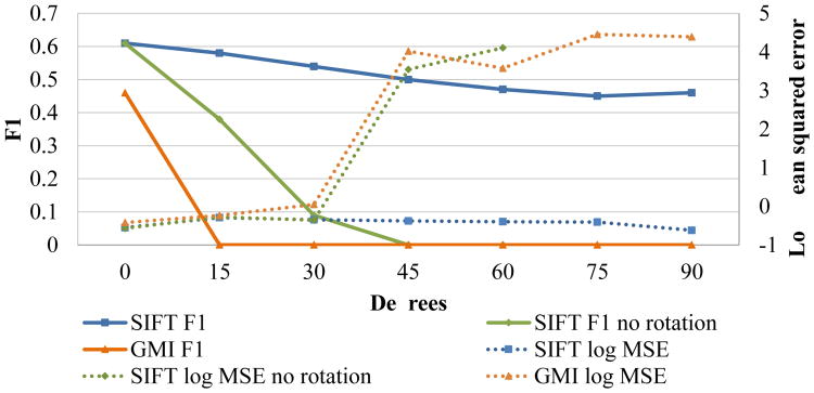
To demonstrate rotation invariance, we performed the same experiment under varying rotation angles from 0 to 90 degrees, using ε = 2 mm. For this test we used the ℓ^∞ neighborhood with the proposed SIFT method, the GMI descriptor, and a modified SIFT descriptor which does not correct for rotation. We condensed the precision and recall into the standard F1 score, reported alongside the mean squared error. We can see in figure 8 that our SIFT descriptor is the only one capable of handling rotations above 30°. This validates the proposed method of orientation estimation, and demonstrates that GMIs are not effective in accounting for rotation when extracted from multiple voxels, which is necessary for accurate matching.

Fig. 8.

MS experiment under varying degrees of rotation.

B. Inter-patient brain MR

This experiment simulates registration of normal brain MRIs from different patients. Among the most common applications of this procedure is brain segmentation. One image, deemed the “atlas,” is labeled by an expert. To segment a second image, called the “subject,” we register it to the atlas. We then assign to each voxel the label of its corresponding atlas location, and compute the standard Dice coefficient between these labels and the ground truth.

To establish ground truth tissue labels, we used BrainWeb simulated MRI images [25]. We chose their “normal brain” model, the same as in section V-A, as the labeled atlas. BrainWeb provides 20 additional anatomical models, which we chose as the unlabeled subjects. All simulations used T1 weighting, 1 mm resolution, 3% noise, and 20% field nonuniformity. To establish a reasonable test for affine registration, we condensed the original BrainWeb tissue classes into three superclasses: brain, background, and other. The brain class consists of gray matter, white matter, and cerebrospinal fluid. The background class consists of empty space. The remaining class consists of all other tissue types, including as skull, muscle and dura mater. The simplified atlas model is shown in figure 9.

Fig. 9.

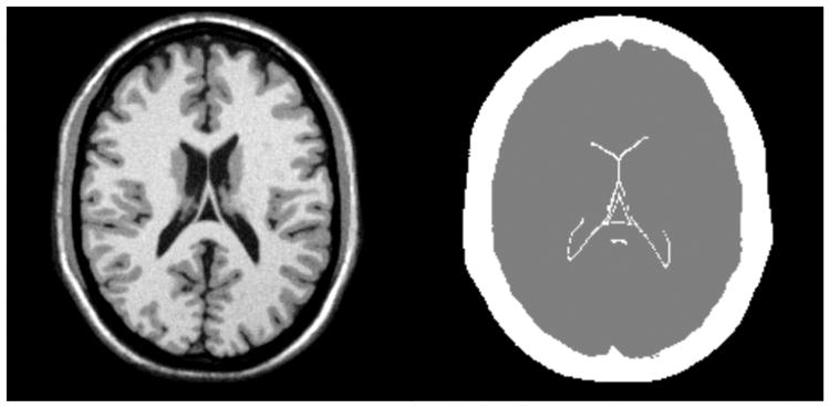
The atlas (left) and tissue model (right) for the segmentation test, showing the background (black), brain (gray), and other (white) classes.

To simulate clinical conditions, we scaled each of the subjects by ±10% in volume, and rotated them by ±10° about the z, x, and z′ axes, in that order, where z′ is the resulting z axis after the second rotation, the origin being the center of the image. The actual transformation parameters were drawn randomly from uniform distributions.

In this experiment we tested several additional methods for comparison to the proposed 3D SIFT-based method. First, we compared to the binary distribution of the 3D SIFT work of Toews et al. [4]. They use a different method for orientation estimation and gradient histograms, a special ranked encoding of the feature vector, and a different matching procedure based on Bayesian probabilities. Second, we compared to intensity-based image registration which iteratively minimizes the mutual information between the reference and the warped image [26]. For this we used the C++ implementation provided by the Advanced Normalization Tools (ANTs) [27]. For the parameters we chose three pyramid levels, each half the size of the next, with an adaptive step size. Registration was performed in four stages: first we compute a translation based on the centers of mass, then we iteratively refine the transformation, first with a translation, then a rigid motion, and finally an affine transformation. The objective function was evaluated at every voxel. These are standard parameters for general-purpose medical image registration. Finally, we computed the scores for the identity transformation, which does no registration at all, to give a sense of the initial misalignment.

As shown in table II, the keypoint-based methods with ℓ¹ neighborhoods outperformed the other methods. We aborted registration if fewer than five inliers were found, which is one more than needed to uniquely determine an affine transformation. Using the ℓ^∞ neighborhood with the proposed 3D SIFT descriptor, sufficient inliers were found in only 13 of 20 cases, whereas the ℓ¹ neighborhood succeeded in all 20 cases. This suggests that the ℓ^∞ neighborhood rejects stable keypoints. Even with the ℓ¹ neighborhood, there may be as few as 50 matches in inter-patient registration, making every true match valuable.

Table II.

Mean Dice coefficients, as percentages. Higher is better.

Method	Brain	Background	Other	Time (s)
SIFT ℓ1	92	96	76	125
GMI ℓ1	92	96	78	380
SIFT* ℓ∞	79	91	54	69
GMI ℓ∞	80	90	54	78
Toews et al.	90	96	74	32
Mutual Information	87	96	69	558
Identity	58	82	28	N/A

^*Average over 13/20 successful cases.

In comparison to the 3D SIFT implementation of Toews et al., the proposed method achieved greater registration accuracy, at the cost of increased computation time. Since we do not have source code for this method, we cannot say with certainty what accounts for its faster processing time. However, three main differences in the methods might explain these results. First, the method of Toews et al. uses a 2 × 2 × 2 array of gradient histograms, with only 8 orientation bins for each histogram. This smaller descriptor should be quicker to compute, and quicker to match between images. Second, their method uses a ranked encoding and Bayesian matching procedure, which might be faster than exhaustive Euclidean matching. Third, their approach did not use the ℓ¹ neighborhood, so it should detect fewer keypoints, possibly with fewer matches, which yields faster matching. In applications where speed is critical, the smaller histogram array, ranked encoding and Bayesian matching could be incorporated into the proposed method.

While the GMI feature descriptors proved less distinctive in the previous experiment, they performed slightly better than the SIFT descriptors in this inter-patient registration task. It is possible that distinctiveness in image representation, which is desirable in intra-patient registration, could actually be a hindrance when the objects being matched have different geometry. To our knowledge, the combination of SIFT keypoints with GMI descriptors is novel, and could be a promising avenue for future research. Nevertheless, with the ℓ¹ neighborhood the SIFT and GMI descriptors yielded very similar registration performance, and the SIFT descriptor was faster to compute.

Interestingly, all of the keypoint-based methods outperformed intensity-based registration in both accuracy and speed. This could be due to the fact that keypoint-based matching is not susceptible to local minima. Another possible reason is that most of the keypoint matches occurred in the brain, while intensity-based registration also accounts for the skull and background. Intensity-based methods might perform better with additional preprocessing. However, ceteris paribus, we ought to prefer methods requiring fewer application-specific adjustments.

C. Abdominal CT from Longitudinal Imaging Studies

The following experiment tests the proposed method on abdominal and full-body CT images from longitudinal imaging studies.

Clinical cases exhibit considerable variation between images, where the same patient is often imaged from different contrast phases and almost always from different scanners. The baseline and followup scans often have different resolutions, e.g. 1 mm slices in the baseline and 5 mm in the followup CT. Accordingly, our dataset consists of 12 cases exhibiting all of these variations. To compensate, our program extracts the resolution from the metadata of each image, accounting for units in all processing stages. For even greater accuracy, at the cost of speed, we interpolate pairs of images to the same resolution prior to keypoint detection. The target resolution is the minimum of the two input image resolutions in each dimension. For example, when registering a 1 × 1 × 1 mm series to one of 0.75 × 0.75 × 5.00 mm resolution, we resample both to a resolution of 0.75 × 0.75 × 1.00 mm, using trilinear interpolation. We report both interpolated and non-interpolated registration accuracy in the following sections.

To establish a reference standard for comparison, we manually annotated the images with fiducial markers. To ensure accuracy and ease of annotation, we marked the centers of three distinct vertebral bodies in each time point, from the eleventh thoracic vertebra, and the second and fifth lumbar vertebrae, as shown in figure 10. We consider the vertebral column an appropriate indicator of abdominal registration performance, as its deformation is sufficiently complex to present a challenge, yet still reasonably approximated by an affine transform. Furthermore, the motion of the spine agrees closely with the motion of the whole torso, which cannot be said of certain soft tissues such as the lungs and diaphragm. Although we took care to mark the center of each vertebral body, human error is inevitable in this task, so our markers are not the ground truth.

Fig. 10.

Fiducial markers for the CT experiment, shown in red.

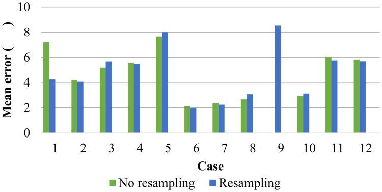
Despite the vast differences in anatomy and resolution, the proposed method performed well on this test, as shown in figure 11. In every case the mean error was below 1 cm, and the mean error across all cases was within 5 mm, as shown in figure 12. We consider this a very good result, as an affine transform is not expected to perfectly model the spine. Furthermore, there is human error in our markers, so we cannot expect a perfect score. This test also demonstrates the value of interpolating the input images prior to registration. While in most cases the method performs equally well with or without resampling, case 9 requires resampling to succeed.

Fig. 11.

Example of CT registration. The baseline (left) has 0.87 × 0.87 × 5.00 mm resolution and shows only the abdomen. The followup (right) has 0.92 × 0.92 × 1.00 mm resolution and shows the full body. The overlay (middle) of the registered baseline (red) and the followup (gray) shows correct spine alignment. The mean landmark error for this case is 8.52 mm.

Fig. 12.

Mean error for the landmarks in each case. Mean error across all cases with resampling: 4.82 mm.

VI. Conclusions

We described a volumetric image registration system based on scale- and rotation-invariant keypoints. Experimental evidence suggests the method performs well in a wide range of image registration tasks, being suitable for registration of intra-patient brain MR in the presence of MS lesions, inter-patient brain MR, and abdominal CT from longitudinal studies. The method outperforms an intensity-based method on these tasks, as well as several other types of 3D keypoints.

We now draw some conclusions on the differences between keypoint-based and intensity-based registration. Intensity-based registration problems are easy to define, but difficult to solve. In contrast, keypoints are difficult to define, but the linear regression problem of section IV-B is trivial to solve. However, keypoint matches usually contain outliers, which must be rejected as in algorithm 1. When the keypoint matches are reliable, these methods should be preferred for their robustness. However, intensity-based methods should be preferred when keypoint matching is unsuccessful, or when the desired geometric transformation is too intricate for keypoints to provide sufficient information. Furthermore, it is difficult to apply keypoint-based methods to multi-modal image registration, as keypoints might not be detected in corresponding locations across modalities. In conventional photography, illumination changes are mostly monotonic, but change of modality in medical imaging is considerably more complex. For example, cerebrospinal fluid appears bright in T2 MRI and dark in T1, while the surrounding brain tissue follows the inverse relationship. Despite these challenges, intensity correlation could be used to match keypoints across modalities, if their locations were reliably detected.

In this work, we have only explored image registration as regression to an affine transform. In practice, this is often the first stage in a larger pipeline, using freeform or spline-based transformations to locally deform the image. The work presented here is relevant in this scenario as well. If the keypoint matches are accurate and well-distributed, they can be interpolated by a thin-plate spline, which is capable of nearly arbitrary deformations. It is also possible to treat keypoint alignment as a non-rigid point-cloud registration problem [28]. Keypoint matches can also be used to guide a non-rigid intensity-based registration algorithm [29]. However, these more advanced methods come with their own share of difficulties. Unlike affine transforms, interpolating splines are highly sensitive to outliers. Furthermore, point-cloud and intensity-based registration are computationally difficult and susceptible to local minima. If these issues were overcome, these techniques could be used to extend the proposed method to a wider range of registration problems.

Appendix

Theorem 1. A point x ∈ ℤⁿ is an extremum of a function I : ℤⁿ → ℝⁿ over its ℓⁱ neighborhood B(x) only if x is a stationary point of its forward differences. Any other neighborhood with this property is a superset of B(x).

Proof: Let e₁,…, e_n denote the standard Euclidean basis vectors. We define the forward differences as ∂I(x)/∂x_k = I(x+e_k)– I(x). We say that x is a stationary point of these differences if ∂I(x)/∂x_k and ∂I(x – e_k)/∂x_k have opposite signs for all k ∈ {1,…n}. That is, the forward difference approximation of the derivative crosses zero in every dimension. Expanding terms, this is equivalent to saying either I(x) > I(x + e_k) and I(x) > I(x – e_k) or I(x) < I(x + e_k) and I(x) < I(x – e_k) for each k. This is satisfied if x is an extremum on the set {x ± e_k : k ∈ {1, …, n}}, which is exactly B(x). It is easy to see that this holds for any superset of B(x), and no other neighborhoods.

Theorem 2. Let x_k ∈ ℝⁿ be a keypoint, and I : ℝⁿ → ℝ be an image. Furthermore, let w : ℝⁿ → ℝ be an (n – 1)-spherically symmetric window about x_k, i.e. w(x) depends only on ‖x – x_k‖. Finally, let the rotation matrix R_I ∈ R^n×n be computed in wI, as defined in section III-B. Then, if $w^{\prime }{I}^{\prime }=w(R_0^T\mathbf{x})I(R_0^T\mathbf{x})$, its orientation has R_I′ = R₀R_i.

Proof: From the chain rule we can compute $\nabla I^{\prime }(\mathbf{x})=R_0\nabla I(R_0^T\mathbf{x})$. Then over w′I′ we have

$$\begin{array}{c}{K}_{I\prime }=\int w^{\prime }(\mathbf{x})\nabla I^{\prime }(\mathbf{x}){(\nabla I^{\prime }(\mathbf{x}))}^{T}d\mathbf{x}\\ =\int w(R_0^T\mathbf{x})(R_0\nabla I(R_0^T\mathbf{x})){(R_0\nabla I(R_0^T\mathbf{x}))}^{T}d\mathbf{x}\\ =R_0(\int w(R_0^T\mathbf{x})\nabla I(R_0^T\mathbf{x}){(\nabla I(R_0^T\mathbf{x}))}^T)R_0^T.\end{array}$$ (16)

The change of variables ${\mathbf{x}}^{\prime }=R_0^T\mathbf{x}$ has a Jacobian determinant of one, so we have

$$\begin{array}{c}{K}_{I^{\prime }}=R_0(\int w({\mathbf{x}}^{\prime })\nabla I({\mathbf{x}}^{\prime }){(\nabla I({\mathbf{x}}^{\prime }))}^{T}d{\mathbf{x}}^{\prime })R_0^T\\ =R_0(R_I\mathrm{\Lambda }{R}_I^T)R_0^T\\ =(R_0{R}_I)\mathrm{\Lambda }{(R_0{R}_I)}^T.\end{array}$$ (17)

Both $R_{I^{\prime }}\mathrm{\Lambda }{R}_{I^{\prime }}^T$, and (R₀R_I) Λ (R₀R_I)^T are eigendecompositions of the matrix K_I′, so we have said in section III-B that R_I′ and R₀R_I can differ only by negation of columns. Let ${\mathit{r}}_i^{\prime }$ and R₀r_i denote the i^th column of each matrix, so either ${\mathit{r}}_i^{\prime }=R_0{\mathit{r}}_i$ or ${\mathit{r}}_i^{\prime }=-R_0{\mathit{r}}_i$. Assume for the sake of contradiction that ${\mathit{r}}_i^{\prime }=-R_0{\mathit{r}}_i$. Then, by construction of ${\mathit{r}}_i^{\text{'}}$ we have

$$\begin{array}{c}1=sgn({\mathit{r}}_{i\prime }^T\int w^{\prime }(\mathbf{x})\nabla I^{\prime }(\mathbf{x})d\mathbf{x})\\ =sgn({(-R_0{\mathit{r}}_i)}^T\int w(R_0^T\mathbf{x})(R_0\nabla I(R_0^T\mathbf{x}))d\mathbf{x})\\ =-sgn({\mathit{r}}_i^T{R}_0^T{R}_0\int w(R_0^T\mathbf{x})\nabla I(R_0^T\mathbf{x})d\mathbf{x})\\ =-sgn({\mathit{r}}_i^T\int w({\mathbf{x}}^{\prime })\nabla I({\mathbf{x}}^{\prime })d{\mathbf{x}}^{\prime })\\ =-1\end{array}$$ (18)

which is a contradiction. Thus ${\mathit{r}}_i^{\text{'}}=R_0{\mathit{r}}_i$, so R_I′ = R₀R_I.

References

- 1.Cheung Warren, Hamarneh Ghassan. n-SIFT: n-dimensional scale invariant feature transform. IEEE Transactions on Image Processing. 2009 Sep;18(9):2012–2021. doi: 10.1109/TIP.2009.2024578. [DOI] [PubMed] [Google Scholar]
- 2.Allaire Stéphane, Kim John J, Breen Stephen L, Jaffray David A, Pekar Vladimir. Full orientation invariance and improved feature selectivity of 3d sift with application to medical image analysis. 2008 IEEE Computer Society Conference on Computer Vision and Pattern Recognition Workshops. 2008 Jun;:1–8. [Google Scholar]
- 3.Ni Dong, Qu Yingge, Yang Xuan, Chui Yim Pan, Tien-Tsin Wong, Ho Simon SM, Heng Pheng Ann. Volumetric ultrasound panorama based on 3d sift. Medical Image Computing and Computer-Assisted Intervention – MICCAI 2008. 2008:52–60. doi: 10.1007/978-3-540-85990-1_7. [DOI] [PubMed] [Google Scholar]
- 4.Toews Matthew, Wells William M., III Efficient and robust model-to-image alignment using 3d scale-invariant features. Medical Image Analysis. 2013;17(3):271–282. doi: 10.1016/j.media.2012.11.002. [DOI] [PMC free article] [PubMed] [Google Scholar]
- 5.Rister Blaine, Reiter Daniel, Zhang Hejia, Volz Daniel, Horowitz Mark, Gabr Refaat E, Cavallaro Joseph R. Scale- and orientation-invariant keypoints in higher-dimensional data; Image Processing (ICIP), 2015 IEEE International Conference on; Sep, 2015. pp. 3490–3494. [Google Scholar]
- 6.Lowe David G. Distinctive image features from scale-invariant keypoints. International Journal of Computer Vision. 2004 Nov;60(2):91–110. [Google Scholar]
- 7.Bay Herbert, Ess Andreas, Tuytelaars Tinne, Van Gool Luc. Speeded-up robust features (SURF) Computer Vision and Image Understanding. 2008 Jun;110(3):346–359. [Google Scholar]
- 8.Rublee Ethan, Rabaud Vincent, Konolige Kurt, Bradski Gary. Proceedings of the 2011 International Conference on Computer Vision. IEEE Computer Society: 2011. ORB: An efficient alternative to SIFT or SURF; pp. 2564–2571. [Google Scholar]
- 9.Kläser Alexander, MarszaŁek Marcin, Schmid Cordelia. A spatio-temporal descriptor based on 3D-gradients. BMVC. 2008;2008 [Google Scholar]
- 10.Scovanner Paul, Ali Saad, Shah Mubarak. A 3-dimensional SIFT descriptor and its application to action recognition. Proceedings of the 15th International Conference on Multimedia; New York, NY, USA. 2007. pp. 357–360. [Google Scholar]
- 11.Rister Blaine. SIFT3D. [accessed June 27, 2017]; Available at http://web.stanford.edu/∼blaine/
- 12.Flitton Gregory, Breckon Toby, Bouallagu Najla Megherbi. Object recognition using 3D SIFT in complex CT volumes. Proceedings of the British Machine Vision Conference. 2010:11.1–11.12. [Google Scholar]
- 13.Lindeberg Tony. Scale-space theory: A basic tool for analysing structures at different scales. Journal of Applied Statistics. 1994:224–270. [Google Scholar]
- 14.Brown M, Lowe D. in Proceedings of the British Machine Vision Conference. BMVA Press; 2002. Invariant features from interest point groups; pp. 23.1–23.10. [DOI] [Google Scholar]
- 15.Sun Xinghua, Chen Mingyu, Hauptmann A. Action recognition via local descriptors and holistic features. 2009 IEEE Computer Society Conference on Computer Vision and Pattern Recognition Workshops. 2009;0:58–65. [Google Scholar]
- 16.Kandel Benjamin M, Wang Danny JJ, Detre John A, Gee James C, Avants Brian B. Decomposing cerebral blood flow MRI into functional and structural components: A non-local approach based on prediction. NeuroImage. 2015;105:156–170. doi: 10.1016/j.neuroimage.2014.10.052. [DOI] [PMC free article] [PubMed] [Google Scholar]
- 17.Lo Chong Hua, Don Hon Son. 3-D moment forms: Their construction and application to object identification and positioning. IEEE Transactions on Pattern Analysis and Machine Intelligence. 1989;11(10):1053–1064. [Google Scholar]
- 18.Harris Chris, Stephens Mike. A combined corner and edge detector. Proceedings of the Fourth Alvey Vision Conference. 1988:147–151. [Google Scholar]
- 19.Dalal Navneet, Triggs Bill. Histograms of oriented gradients for human detection. CVPR. 2005:886–893. [Google Scholar]
- 20.Coexeter HSM. Regular Polytopes. 3. Dover Publications, New York; New York: 1973. [Google Scholar]
- 21.Scovanner Paul, Ali Saad, Shah Mubarak. 3D SIFT. [accessed June 27, 2017]; Available at http://crcv.ucf.edu/source/3D.
- 22.Möller Tomas, Trumbore Ben. ACM SIGGRAPH 2005 Courses. ACM; 2005. Fast, minimum storage ray/triangle intersection; p. 7. [Google Scholar]
- 23.Shen Dinggang, Davatzikos C. Hammer: hierarchical attribute matching mechanism for elastic registration. IEEE Transactions on Medical Imaging. 2002 Nov;21(11):1421–1439. doi: 10.1109/TMI.2002.803111. [DOI] [PubMed] [Google Scholar]
- 24.Fischler Martin A, Bolles Robert C. Random sample consensus: A paradigm for model fitting with applications to image analysis and automated cartography. Communications of the ACM. 1981 Jun;24(6):381–395. [Google Scholar]
- 25.Cocosco Chris A, Kollokian Vasken, Kwan Remi KS, Bruce Pike G, Evans Alan C. Brainweb: Online interface to a 3D MRI simulated brain database. NeuroImage. 1997;5:425. [Google Scholar]
- 26.Pluim Josien PW, Maintz JB Antoine, Viergever Max A. Mutual information based registration of medical images: A survey. IEEE Transactions on Medical Imaging. 2003;22(8):986–1004. doi: 10.1109/TMI.2003.815867. [DOI] [PubMed] [Google Scholar]
- 27.Avants Brian B, Tustison Nick, Song Gang. Advanced normalization tools (ANTs) Insight Journal. 2009;2:1–35. [Google Scholar]
- 28.Nguyen Thanh M, Wu QM Jonathan. Multiple kernel point set registration. IEEE Transactions on Medical Imaging. 2016 Jun;35(6):1381–1394. doi: 10.1109/TMI.2015.2511063. [DOI] [PubMed] [Google Scholar]
- 29.Han Xiao. EMPIRE10: MICCAI 2010 Workshop on Evaluation of Methods for Pulmonary Image Registration. Vol. 2010. Beijing: Sep, 2010. Feature-constrained nonlinear registration of lung ct images. [Google Scholar]