How to deal with parameters for whole-cell modelling

Abstract

Dynamical systems describing whole cells are on the verge of becoming a reality. But as models of reality, they are only useful if we have realistic parameters for the molecular reaction rates and cell physiological processes. There is currently no suitable framework to reliably estimate hundreds, let alone thousands, of reaction rate parameters. Here, we map out the relative weaknesses and promises of different approaches aimed at redressing this issue. While suitable procedures for estimation or inference of the whole (vast) set of parameters will, in all likelihood, remain elusive, some hope can be drawn from the fact that much of the cellular behaviour may be explained in terms of smaller sets of parameters. Identifying such parameter sets and assessing their behaviour is now becoming possible even for very large systems of equations, and we expect such methods to become central tools in the development and analysis of whole-cell models.

1. Introduction

John von Neumann was famously dismissive of over-eager curve-fitting. ‘With four parameters I can fit an elephant, and with five I can make him wiggle his trunk’ encapsulates his position [1], and is a view shared by many. However, computational science is now exploring models of great complexity with hundreds and even thousands of parameters—and it is perhaps fitting that one of von Neumann's many great legacies, the modern computer, is enabling this; whole-cell models (WCMs) are perhaps the most ambitious example of large-scale models in the life sciences and here we discuss the statistical and parameter estimation challenges intrinsic to such efforts.

Mathematical models can have manifold uses in biology. First and foremost, they show that complexity can arise even from very simple dynamical systems [2]. At their best, such simple models capture essential aspects of biological systems and afford us with fundamental new insights. Lotka–Volterra models in ecology, the Wright–Fisher model in population genetics, Turing [3] and French-flag [4] models in developmental biology [5], the repressilator in synthetic biology [6] and the standard model of gene expression [7] in molecular biology are all examples of powerful yet simple models that have substantially contributed to our understanding of biological processes from the molecular to the eco-system level.

Despite the simplicity of these models—often to the extent that substantial and non-trivial analytical solutions are available for key aspects of their behaviour—their validity or relevance has been probed and demonstrated repeatedly. Models are not reality, nor are they meant to represent all aspects of reality faithfully [8]. Nevertheless, these simple models have essentially framed how we understand many key biological processes, and can serve as useful guides as to how we should best explore them in more detail. However, such models are quickly found wanting when more detailed data become available, or when related but more complicated processes are studied. For example, spatial structure is known to affect the validity of both ecological and population genetic processes, and at the very least models have to be modified to account for these changes. As models become more complex and incorporate often complex feedback structures [9,10], we can no longer rely on analytical techniques, and instead start to require computer simulations to explore their behaviour.

1.1. From simple to complex models

Some models aim to capture the essential hallmarks of life—such as metabolism, nutrient uptake, gene expression regulation and replication—but in a simplified representation that does not aim to replicate the true complexity of a whole organism [11–16]. These coarse-grained models have shown great promise and allow us to integrate molecular, cellular and population level/scale processes into a coherent—and analytically tractable—modelling framework. While real cells will be much more complicated, these simple model systems have successfully provided insight into fundamental cell physiology, e.g. processes affecting microbial growth rates [12,13,15,16].

Increasingly, there is interest in generating more realistic and complicated models that, rather than aiming to provide abstract representations of key features, incorporate extensive details of known components and interactions (or reactions) present in a system. In cell biology, for example, there are now numerous attempts at modelling aspects of metabolism, gene regulation and signalling at cellular level [17–24]. Perhaps the best established are metabolic models, where a powerful set of tools, based around flux balance analysis (FBA) [25], allows us to explore metabolic phenotypes in silico at a genomic level for an increasing range of organisms (and some individual cell types) [24,26,27]. However, such models are stoichiometric and thus give us information about biochemical reaction schemes and fluxes, but not details about the system dynamics.

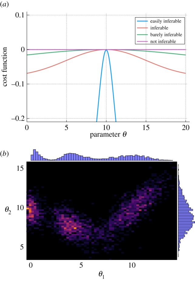
Advances in both high-throughput experimentation and computational power have opened up the possibility of creating and analysing more complex dynamic models of biological systems, including many which represent processes occurring at different scales [28,29]. Numerous models now face the challenge of being large (in terms of numbers of species and parameters represented), multi-scale and/or hybrid in nature (incorporating multiple different mathematical representations) [23,28–30]. The most ambitious models to date—the WCMs—aim to provide faithful in silico representations of real biological cells, including all major cellular processes and components, and are both very large scale and hybrid (figure 1) [31–33].

Figure 1.

WCMs. Genome-scale models of metabolism and gene regulation exist for many important model organisms. WCMs now try to combine these, together with any available detailed models about, for example, signalling networks and basic biophysical models of cellular processes and structure, and molecular machines into a single coherent simulation platform. For this, we will typically rely on hybrid modelling approaches, that combine different modelling approaches, which reflect the quality and amount of data available for different aspects of the cell's behaviour.

There are several potential uses for such WCMs:

• (1) To gain mechanistic insights, by serving as an in silico ‘blueprint’ through which we study the behaviour of real cells.

• (2) As a rational screening and predictive tool, to explore in silico what might be hard or impossible to study in vivo.

• (3) To drive new biological discoveries, by showing where we lack sufficient understanding, and identifying promising future directions to pursue experimentally.

• (4) To study emergent phenomena which are only apparent when we consider a system as a whole.

• (5) To integrate heterogeneous datasets and amalgamate our current knowledge into a single modelling framework.

• (6) Perhaps eventually to study, via virtual competitions between different cell architectures, evolutionary dynamics in unprecedented detail (but at enormous, currently crippling, computational cost).

• (7) In the meantime, as the community strives to develop viable WCMs, the technological, computational and statistical challenges of model building will, no doubt, give rise to much fruitful research and re-usable methodology.

Here, we focus on the inference and statistical modelling challenges inherent to developing WCMs (and other complex models), in terms of model construction, parameter estimation, uncertainty and sensitivity analyses, and model validation and refinement. Some of these are generic modelling challenges—but worth reiterating—while others are specific to large-scale, multi-scale and hybrid models.

2. Combining models

The first example of a comprehensive WCM, published in 2012, describes the life cycle of a simple bacterium, Mycoplasma genitalium, accounting for the functions of all 525 known annotated genes [31]. This model was constructed by combining 28 submodels that describe cellular processes, including metabolism, gene expression regulation, protein synthesis, biomolecule assembly, signalling and cell division functions. Such a hybrid model requires a sophisticated and non-trivial simulation framework, as the different modelling modalities required, e.g. for FBA and stochastic gene expression, need to be reconciled with one another and staged appropriately such that cell–physiological processes are realistically scheduled.

For some of the obvious next candidates to generate WCMs, such as Escherichia coli or Bacillus subtilis, we already have vast amounts of metabolomic, transcriptomic and proteomic data, as well as knowledge summarized in databases. There are, for example, the genome-scale metabolic models that we have already touched upon above. These are complemented by gene regulation and protein–protein interaction networks that capture interactions that have been experimentally substantiated to different degrees. Construction of the next WCMs will probably follow similar approaches that combine existing submodels; the challenge is to (i) construct and parametrize appropriate submodels and (ii) intercalate these networks to enable computational analyses. An even more ambitious goal is to extend such approaches to study eukaryotic species such as Saccharomyces cerevisiae or mammalian cells, where not only do we have to deal with much larger genomes, but features such as subcellular compartments and more complex regulatory mechanisms.

Approaches and difficulties relating to submodel construction and parametrization are discussed in subsequent sections, but even once we have extensively characterized, carefully parametrized and validated models describing different aspects of a complete system, combining these will remain a formidable challenge [28,29,34]. Submodels were successfully integrated in the original WCM by assuming independence on short time scales, and defining a collection of cell variables that could be shared among the various distinct cellular processes [31]. However, we should bear in mind the difficulties faced in other scientific fields, where complex systems are frequently studied using multi-scale [29] and multi-physics modelling approaches [35]. In climate modelling, for example, multi-physics approaches combine models of atmospheric chemistry with models of ocean currents, which are then coupled, using, for example, partial differential equations. But in those cases the processes of connecting the different subsystems can introduce uncertainty and bias, as the feedback between different constituent parts of the larger system can also be complicated, and coupling different systems requires considerable fine-tuning of the equations linking the different subsystems.

It will be crucial to develop ways to assess how uncertainties and errors may be propagated through a complex model. Any inaccuracies in linking different submodels can severely compromise the compound model, irrespective of how carefully the submodels have been calibrated and tuned. We should also consider how else we can incorporate the impact of cellular context when modelling subsystems. The notion of extrinsic noise was introduced precisely to account for cell-to-cell heterogeneity in factors that are not explicitly captured by a model, but which may differ between cells [36]. Frequently, it is possible to capture the leading effects of such extrinsic factors by allowing for differences in the rate parameters between cells [37–39].

3. Parameter estimation

The models, f(Y; θ, t), we are after capture the behaviour of our organism/cell, or all of its constituent parts subsumed in the vector, Y, over time, t; θ denotes the vector of parameters (e.g. rate constants for metabolic and kinetic processes). Depending on the nature of the process being studied, and the level of knowledge we have about a system, we may require different modelling formalisms (e.g. deterministic, stochastic, logical or stoichiometric); frequently, we will make use of ordinary differential equations of the form

3.1

where ξ(Y, t) is an optional additional term to denote stochastic processes (e.g. due to random timings of collisions between molecules in the cellular interior).

The structure of the model—in terms of the mathematical representation of the function f(Y; θ, t) which describes the system components and relationships—is defined according to our current knowledge, perhaps in combination with data-driven network inference techniques that aim to learn the likely structure of a system from observations of its variables [40–46]. However, we also need to obtain suitable estimates for the parameters, either from experimentally determined values or by using statistical approaches to estimate (or infer) these values by fitting model simulations to observed data.

3.1. Experimental estimates

The authors of the first WCM [31], and others [47], stress the need to only use experimentally measured parameters in biological models. This may appear a rigorous way to ensure that a model is properly calibrated against the available information, and that free (wiggle) parameters are avoided. There are, however, a number of pitfalls to such a strategy [48,49].

First, the mathematical models that we are considering are abstractions of much more complex processes (even within WCMs that attempt to incorporate functions of all known genes); therefore, the meaning of a parameter needs to be carefully evaluated in each case. For example, Michaelis–Menten kinetics are frequently used to model enzymatic reactions, but these model assumptions may be far removed from the true biophysical processes occurring inside a crowded cellular environment, and may grossly simplify the complex catalytic regulation that occurs in the real system. The model parameters may therefore not really reflect the biophysical constants that are experimentally accessible using in vitro or in vivo assays.

Second, biochemical reaction rates depend on numerous environmental (e.g. temperature, acidity, ionic strengths) and cellular (e.g. viscosity, allosteric regulation) factors. While we can aim to design experiments so that our measurements are as relevant as possible [50–53], few biological parameters can be measured precisely in their appropriate in vivo context. We are often forced to resort to parameter estimates obtained from in vitro assays or from other (related) species, but there are good reasons to be wary of such estimates: the thermodynamic and ecological differences can lead to pronounced differences between, for example, catalytic rates; similarly, differences in the architecture of the cell membrane and embedded transporters and receptors can affect transport as well as cell–environment interactions.

Third, any modelling using fixed parameters ought to be viewed with a healthy dose of scepticism: uncertainty and noise pervade all of cell biology, and failure to account for this appropriately can compromise analyses and further uses of the resulting model [48]. Such shortcomings may not necessarily be detectable in validation experiments—particularly when dealing with such complex models, numerous parameter combinations may provide a reasonable match to the data [54], yet the complexity renders these models intractable to existing approaches designed to identify these situations.

Finally, not all relevant parameters may be known (even when we include data from related species) and, in some cases, may not be experimentally accessible. A key advantage of modelling is that it enables us to explore the influence of processes that we cannot directly observe, by linking these processes in a mathematical framework to variables we can probe experimentally. If we restrict our models to only include parameters that we can estimate experimentally, we surely risk biasing our models (and thus conclusions) according to our current experimental limitations.

Ideally, we should make use of in vivo data from the target organism of interest where available to help estimate parameters in the correct cellular context. However, we should also exploit the diverse array of techniques available that allow us to infer the most probable parameter values from the observed behaviour of a system.

3.2. Statistical inference

Here by inference we mean the use of sound statistical methods to learn the parameter and, where possible, include an explicit assessment of the associated uncertainty. The likelihood is a central quantity for such methods [55]; it is defined as the probability of observing the data 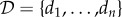given a parameter, θ,

3.2

Here Pr(d | θ) is the probability of an experimental observation, d, given the mathematical model f(Y; θ, t), for a given value of θ. Note that θ will for all interesting problems, including WCMs, be a vector containing all the model parameters.

The maximum-likelihood estimate (MLE) of θ, denoted by , is obtained by varying θ until the likelihood becomes maximal

3.3

and it is the best estimate of θ given the data, , and the assumed model, f(Y; θ, t). Frequentist inference approaches aim to identify the MLE of θ; for most non-trivial biological models, we expect the likelihood surface (the likelihood function evaluated over the parameter space) to be complex and multi-modal in nature and we thus rely on numerical optimization algorithms rather than analytical approaches to find the maximum. Local optimization algorithms risk identifying local maxima, so there is strong reason to prefer global optimization approaches that aim to explore the parameter space more broadly [56,57]. For sufficiently simple models (those where the likelihood function in concave around a single maximum), even global uncertainty statements can be made. Experience suggests that this latter case is the exception rather than the rule for dynamical systems in cell and molecular biology [54,58]. Some approaches, such as profile-likelihood methods, try to assess the uncertainty for each parameter [59,60], which may hold particular appeal for those interested in inferring specific parameters with accuracy.

The likelihood is also used in Bayesian inference where it is combined with the prior π(θ)—a probability over the parameter space that reflects the level of existing knowledge (or lack thereof)—to arrive at the posterior distribution

3.4

Here now, instead of providing a single estimate (plus potentially associated confidence intervals), we specify the probability distribution over the whole potential parameter space considered, Ω_θ. We can, if preferred also choose to report a point estimate, i.e. 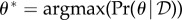, for pragmatic reasons, but typically we find it preferable to consider the whole posterior distribution (at least conceptually).

The Bayesian framework offers considerable interpretational advantages over the traditional likelihood approach (reviewed elsewhere [61]), but comes, in its full form, with a computational burden that can prove prohibitive. Generally, for any half-way realistic model the denominator in equation (3.4) will be hard to evaluate (hence the need for Markov chain Monte Carlo and related methods in Bayesian inference). For many scientifically interesting problems, even evaluation of the likelihood is computationally unfeasible and a range of methods, including approximate Bayesian computation and other likelihood-free inference methods have risen to prominence [62–65], which extend the applicability of the Bayesian framework to problems that have computationally intractable likelihood functions.

3.3. Application to large-scale, hybrid models

For WCMs (and other large-scale, hybrid models), we will require further advances and improvements in both experimental techniques, and computational and statistical methods in order to ensure that these models are built on solid foundations.

Despite the wealth of ‘omics’ level data available for the most well-studied organisms, e.g. E. coli and S. cerevisiae, we still lack the comprehensive in vivo measurements needed to allow us to obtain the relevant parameter estimates in a systematic and automated way. The original M. genitalium WCM relied on the authors painstakingly compiling information from over 900 publications in order to parametrize the model (despite purposefully choosing a fairly small organism for their proof-of-concept study) [31]. To enable development of such complex biological models to become more mainstream will require community-wide efforts to establish accepted tools and standards for collating and annotating data from heterogeneous sources [66–68] as well as improved means of harvesting existing literature and data sources [23,69]. New experiments can expand the coverage of existing datasets and ensure consistency in terms of experimental conditions [70], as well as providing us with a better understanding of the relationships between in vivo and in vitro parameter estimates (these may differ by several orders of magnitude, thus in vitro estimates can be misleading) [71].

At present, none of the statistical inference methods outlined above are applicable at the scale of WCMs. However, smaller subsystems, such as individual pathways, regulatory motifs, receptor complexes or systems comprising small sets of metabolic reactions and the associated regulatory processes can be effectively parametrized using such methods [72]. For such systems, we can often estimate parameters, including uncertainty; and we are frequently able to assess parameter sensitivity (typically measured as the change in some model output, e.g. predicted protein abundance, in response to varying a single parameter). In some cases, experimental measurements of species concentrations may allow us to effectively decompose our models into smaller modules for efficient parameter estimation [73]. Bayesian inference methods in particular are limited in terms of scale and are generally only feasible for models with up to tens to hundreds of species and parameters [74,75]. Some optimization approaches are much more scalable though, with recent advances allowing parametrization of ODE models comprising hundreds to thousands of species and parameters [65,76,77]. As always, however, the chance of being trapped in local optima is high for such large-dimensional problems.

A combination of both inference and experimental estimation will probably be needed to parametrize complex biological models. It is currently impractical to use inference techniques within the context of a full WCM, unless considering very small pre-defined subsets of the parameters and, even then, the computational costs are enormous [67]. We can, however, make use of scalable inference techniques [78] to help us parametrize the component submodels, using experimental information where available as prior knowledge for the inference procedures. This will allow us to avoid some of the potential pitfalls outlined above of experimental estimates, and generate parameter estimates that take into account—to the best of our ability—the influences of cellular and system context, and make use of the most appropriate in vivo datasets. Crucially, rigorous statistical inference also enables us to explore the relationships between model parameters and start to understand and quantify the uncertainties inherent to any mathematical model.

4. Model and parameter uncertainty

There are uncertainties in both the structure and parameters associated with any mathematical model of a biological system. We often do not know the exact components and interactions that make up a given subcellular system (such as signalling or metabolic pathways) and, in particular, the crosstalk that occurs between such pathways. We necessarily use abstract and simplified mathematical representations of the dynamics, and frequently rely on phenomenological models, rather than modelling the fundamental physical and chemical processes that occur in the cell. For example, when modelling enzymatic reactions or gene regulation at a large scale, we often rely on Michaelis–Menten kinetics—even when the assumptions behind this modelling formalism do not hold (e.g. assumptions of irreversibility and time-scale separations)—or Hill kinetics, the latter of which has no established mechanistic interpretation [79,80]. Even when we attempt to include molecular details of the complete system (such as in a WCM) we are still forced to ignore many of the true complexities of the processes occurring, e.g. post-translational modifications or complex regulation of enzymatic reactions, as it is simply infeasible to represent these in such a large model.

4.1. Structural uncertainty

The structural and mechanistic assumptions inherent to our chosen model will influence the conclusions and predictions we draw. While uncertainties in parameter values are generally acknowledged and explored to some extent, structural uncertainty—the inherent ambiguity as to the ‘correct’ (least wrong) structure of the mathematical model—is often overlooked. However, there are methods we can use to explore how our choices about model definition—in terms of the system components we include, and the way we represent these mathematically—may be influencing our conclusions.

Model selection methods enable us to compare several proposed models (which correspond to our different hypotheses about a system) and determine which are best supported by the available data. Depending on the nature of the set of models, there are a range of methods available to rank our models within both frequentist or Bayesian inference frameworks—e.g. likelihood ratio tests, Akaike's (or other) information criterion, Bayes factors, or estimation of the marginal likelihood (the denominator in equation (3.4)) [81]. We can either choose to select the best-ranked model for our analyses, or use model averaging techniques to generate conclusions from a pool of models, with their relative contributions weighted according to how well they fit the observed data [82,83].

Increasingly, there are techniques that enable us to consider a collection of good models when making predictions or drawing conclusions. Particularly when working with data-driven models (i.e. inferred network structures consistent with the data), we can consider the model structure within a probabilistic framework, rather than assuming a fixed model structure before making predictions [84,85]. We can explore the robustness of our model predictions—whether the conclusions we draw are consistent across a set of good models, or whether they rely on one specific set of model assumptions [86,87]; in the latter case, we may want to be wary of such conclusions if we cannot be confident in the validity of those assumptions. Ensemble modelling approaches—which analyse the behaviour of a population of distinct models—have been central to the success of model predictions in other fields, e.g. climate forecasting, by allowing us to understand and quantify the uncertainties in our conclusions [88]; such methods are starting to be applied to biological models [42,89–91]. In situations where we cannot be sure of the best choice of model (even when using model selection techniques) and many scenarios are consistent with the available data, it is crucial to understand how much our assumptions may be influencing our results.

Although such techniques are not currently feasible to apply to WCMs, we should make sure that we consider these issues when constructing the constituent submodels, and when deciding what components we should include in our system, and how we represent these mathematically. It should be clear, however, that any WCM, no matter how carefully it has been constructed, will be subject to considerable structural uncertainty. That also means that there will be a potentially large number of model modifications and alternative models that will be equally capable of describing available data; and make essentially indistinguishable predictions about the system behaviour in many cases.

4.2. Parameter uncertainty

Regardless of how we estimate our parameters—whether through experimental determination or statistical inference—there will be some degree of uncertainty in the resulting values. In all cases, it is important to quantify the level of this uncertainty and, ideally, consider the relationships between model parameters, as well as determining to what extent these uncertainties influence our conclusions.

For experimental estimates, we face the difficulties discussed earlier in terms of how to best approximate the true cellular environment when carrying out measurements; there will be uncertainties in the methods we use for quantification; and of course many sources of environmental and cellular heterogeneity, only some of which we can control. With inferred parameter estimates, we again rely on observed experimental data (with their associated uncertainties) but also need to consider the limitations of the specific inference method we use. Particularly as models get larger, we are also likely to face issues around identifiability [42,77,92]. Structural identifiability is a property of the model structure and considers whether this allows us to uniquely determine the parameter values from system observations (assuming ideal conditions and data). This is a prerequisite for practical identifiability, which is dependent on the data available and whether these are sufficient to allow parameter determination (i.e. this reflects the information content of the data). Assessing these properties can help us modify our model structure and/or experimental design to deal with lack of identifiability [50,93].

For models parametrized with point estimates (single values for each model parameter), we can use sensitivity analyses to explore the impact of uncertainty in those estimated values. Sensitivity analysis determines how uncertainties in a model's inputs (e.g. parameter values or initial conditions) contribute to uncertainty in the output of the model (e.g. simulated dynamics) [58,94,95]. To perform a parametric sensitivity analysis, we perturb a single parameter—or better, combinations of parameters—and test how much this affects our model output, e.g. simulations of system dynamics. This allows us to quantify (to some extent) how the uncertainties and potential errors in our parameter estimates might propagate through our modelling analysis. Ideally, if we have assigned confidence intervals to our parameters (e.g. by estimating the potential magnitude of errors in our experimental measurements, or inferring confidence intervals along with point estimates in a frequentist framework) we can test the influence of perturbations of these magnitudes. The simplest methods—perturbing each parameter in turn—ignore potential dependencies between parameters, yet these may be strongly correlated, so ideally we should explore the multi-dimensional parameter space in more detail using global rather than local sensitivity analyses. However, this is of course computationally very demanding, particularly as models increase in size and complexity, and stochasticity becomes important.

Bayesian inference methods provide us with far more information as they allow us to infer the full, joint posterior probability distribution for the model parameters. This not only gives us details about the uncertainties in single parameters (from the shapes of the marginal probability distributions), but also allows us to see the full dependencies between different model parameters—allowing us to, for example, detect groups of parameters that can vary in coordinated ways while still providing a good match between model simulations and observed data (figure 2). The joint posterior distribution therefore provides a comprehensive assessment of the uncertainties in our inferred parameter values (albeit these are, of course, like any parameter estimates dependent on the structural assumptions made in our model). To understand how these uncertainties influence our conclusions, we can sample probable point estimates from the posterior distribution and compare the results obtained from our model using these different combinations of parameters—i.e. generate posterior predictive distributions.

Figure 2.

Parameter inference. (a) The precision with which the parameters/rate constants of dynamical systems can be inferred varies greatly. For some parameters, it is possible to estimate them with low levels of uncertainty given present information, whereas others are very hard to estimate; for the flattest cost-function/likelihood surfaces/posterior distributions the variability overwhelms the mean; here even experimental measurements may be subject to unacceptably high levels of uncertainty. A flip-side of this is that the parameters which are hard to infer are also those that affect the system's behaviour least. (b) Instead of looking at the distributions over parameter estimates for individual parameters (e.g. θ₁ and θ₂) we should consider their joint distributions (again, we can characterize the behaviour of, for example, likelihood and posteriors similarly). These joint distributions also provide an opportunity to study the robustness of the WCM behaviour.

The M. genitalium WCM was parametrized using experimentally derived point estimates [31]. These are of course subject to uncertainties to various degrees—and, during model refinement, several parameters needed to be updated in order to reduce discrepancies between model simulations and data observations. However, with such a complex model, we expect there to be strong dependencies between model parameters, so the refined estimates will always be conditional on the fixed values assumed for all other model parameters (which are of course also subject to uncertainty). Modern sensitivity and robustness analysis methods (e.g. [96,97]) may come to the rescue here and allow us to assess and mitigate parametric uncertainty even for models with many parameters.

Bayesian methods, while providing the richest information, are generally only feasible to apply to relatively small-scale models (e.g. tens to hundreds of species and parameters) due to the computational demands of these methods. Similarly, methods to assess identifiability of models and to characterize the impact of parameter uncertainties tend to be limited to similar size models, although some more recent developments can deal with slightly larger scale models of a few hundred parameters [92,98]. Of course, such methods are currently not compatible with the size and complex hybrid nature of WCMs. However, using these approaches to quantify parametric uncertainty in smaller scale constituent submodels, and assessing the impact that this has on our model conclusions, will allow us to be more confident in the quality of the WCM components.

Overall, a host of recent analyses have shown that from an estimation/inverse problem perspective it is important to focus on the joint distributions over parameters, which cannot be fully understood by looking at the uncertainties associated with individual parameters. If we have two parameters, θ₁ and θ₂, with high uncertainties (whether this is expressed by broad marginal posteriors, flat likelihoods, flat profile-likelihoods, or some other flat cost function), once one of them, e.g. θ₁, is known we may already have a very good idea as to what the value of θ₂ is going to be. Such conditional certainty in the presence of otherwise considerable (marginal) uncertainty appears to be a hallmark of many dynamical, including stochastic, systems [96,99].

In this context, the notion of sloppy models has gained some notoriety/prominence [100]. But statistical inference provides a natural framework in which such issues can be resolved straightforwardly: issues such as sloppiness and identifiability notwithstanding, the sets of parameters that affect system behaviour profoundly will be inferred relatively easily [101,102]. By contrast, parameters that are hard to infer exert less influence on the system's dynamics. A crucial question in this context is how many parameters fall into the two categories, of inferable and non-inferable parameters. For small systems (up to 60 parameters) typically one-third of the parameters are inferable using conventional likelihood criteria, and they suffice to understand and model the system dynamics [58]. Exploring such high-dimensional and complex posteriors is challenging, especially when visual inspection becomes unfeasible or at least problematic. Principal component analysis on posterior samples [63], or use of the Fisher information matrix [96,99]—which quantifies uncertainty in parameter estimates—offer potential routes, e.g. to identify those parameters that exert the greatest influence on system dynamics.

Two caveats are in order at this stage: (i) stitching different smaller and well-parametrized models together to form a single integrated model is likely to introduce complicated correlation structures among the set of parameters in the model which deserve closer attention and (ii) the parameters of an incorrect model may be inferred with relative precision. It is therefore important to consider both structural and parametric uncertainty in every biological modelling study. Scaling such approaches up to WCMs will be a technical challenge and require the development of suitable approximations, or potentially emulation or surrogate modelling approaches [28,103,104].

5. Model improvement and validation

Mathematical models represent our best current understanding and representation of the true biological systems. We should aim to continually refine and improve them as new data become available and we gain knowledge about the underlying systems. Model selection methods, outlined above, allow us to propose several alternative mechanistic representations and select those that are best supported by the available experimental data [81,82]. There are also experimental design approaches that aim to identify the most informative experiments to perform in order to improve our models and distinguish between different hypotheses or reduce uncertainty in parameter estimates (figure 3) [50–53,105]. Iterative cycles of model prediction, experimental data collection and model refinement enable us to gradually improve models—using well-targeted experiments—and gain mechanistic insight into a given system [53,75,93].

Figure 3.

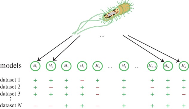
Model selection and model checking: owing to structural as well as more general uncertainty, there will typically be many alternative models that can describe the same behaviour. To test which of these (structurally different) candidate WCMs, M₁, M₂, …, M_N, best describes reality, we cannot merely rely on available data. Instead we will typically only be able to distinguish between such candidates when using data from carefully designed, discriminatory experiments. Owing to the complexity of the problem—the number of potential plausible models probably vastly exceeds our financial and material resources to test them—we may expect that several models could agree with all of the available test datasets.

Again, such methods are currently not extendable to the scale and complexity of WCMs, but could—and should—be used to rigorously test, improve and validate smaller subsections of the complete model. In fact, to refine some of the parameter estimates in the M. genitalium WCM, reduced versions of the model were constructed in order to make it feasible to apply numerical optimization techniques [31,68]. This WCM was validated by comparing model predictions to several independent experimental datasets, and subsequently used to predict the response of the bacterium to various perturbations (in the form of single-gene mutations) [31,33]. Comparing model predictions to experimental data from various mutant strains identified several discrepancies, which could then be explored in more detail to identify aspects of the model—in this case parameter values—that required updating (and were later shown to be consistent with new experimental measurements).

Despite these successes, these improvements and refinements to the model are fairly ad hoc. For the development of large-scale, hybrid models to become more established and reliable, we need to develop more systematic and automated ways to test and refine these models, particularly when attempting to extend WCMs to more complex organisms and cells [68,106,107]. At present, we cannot identify how much we should trust different aspects of such models, which parts of the model require improvement, and how uncertainties and errors in the model structure and parameters (which are, to some extent at least, inevitable) may be influencing any conclusions drawn from the model.

6. Conclusion and outlook

The first comprehensive WCM is an impressive demonstration of how to successfully integrate many large and diverse submodels, and heterogeneous experimental data, into a single cohesive modelling framework. It demonstrates the feasibility, and potential utility, of developing far more complex and intricate models than are currently widely used in systems, cell and molecular biology. However, we need to be aware of the limitations and uncertainties associated with such models, particularly given that many of our established techniques for developing, validating and refining mathematical models simply cannot be applied at these scales.

Extensive analyses of smaller scale models have repeatedly demonstrated that uncertainties in both model structure and parameters are prevalent. Often, numerous models will be able to fit the observed data—even when dealing with very small systems—yet the predictions and conclusions we would draw from these models can differ substantially. Methods for constructing, parametrizing, refining and quantifying uncertainties in models are steadily becoming more scalable. They still, however, fall far short of being applicable at the scale of WCMs, but can be used to rigorously analyse and test the constituent parts that are included in such models. This will not overcome our lack of knowledge about uncertainties within the complete model, but at least can contribute to improving the quality of, and assessing the validity of the assumptions underlying the component submodels.

We should not overlook the roles that models at different levels of abstraction and complexity can play in advancing our understanding of biological systems. Despite the fact that WCMs attempt to represent all cellular components and processes, they still rely on simplified representations of the true processes, and are necessarily biased towards our current understanding. Of course, in some cases, we will need to consider the cellular context and larger system that a biological process is embedded in, in order to explain our observations. However, smaller models that are amenable to the diverse and powerful array of modelling techniques available are much better suited to provide us with detailed mechanistic insight. Using these tools, we can rigorously explore and compare potential hypotheses, quantify the uncertainties associated with our model inputs and outputs, and improve our understanding of complex biochemical processes and regulatory mechanisms occurring within a cell. Without a thorough assessment of our (un)certainty regarding their fundamental dynamical determinants, WCMs would risk representing little more than sophisticated databases that offer few computational advantages compared with models that are slightly less complex but more amenable to existing statistical and computational tools.

Data accessibility

This article has no additional data.

Authors' contributions

A.C.B. and M.P.H.S. contributed equally to conception and writing of this review.

Competing interests

We declare we have no competing interests.

Funding

A.C.B. is a BBSRC Future Leader Fellow.

References

- 1.Dyson F. 2004. A meeting with Enrico Fermi. Nature 427, 297 ( 10.1038/427297a) [DOI] [PubMed] [Google Scholar]
- 2.May R. 1976. Simple mathematical models with very complicated dynamics. Nature 261, 459–467. ( 10.1038/261459a0) [DOI] [PubMed] [Google Scholar]
- 3.Turing AM. 1952. The chemical basis of morphogenesis. Phil. Trans. R. Soc. Lond. B 237, 38–72. ( 10.1098/rstb.1952.0012) [DOI] [PMC free article] [PubMed] [Google Scholar]
- 4.Wolpert L. 1969. Positional information and the spatial pattern of cellular differentiation. J. Theor. Biol. 25, 1–47. ( 10.1016/S0022-5193(69)80016-0) [DOI] [PubMed] [Google Scholar]
- 5.Green JBA, Sharpe J. 2015. Positional information and reaction-diffusion: two big ideas in developmental biology combine. Development 142, 1203–1211. ( 10.1242/dev.114991) [DOI] [PubMed] [Google Scholar]
- 6.Elowitz MB, Leibler S. 2000. A synthetic oscillatory network of transcriptional regulators. Nature 403, 335–338. ( 10.1038/35002125) [DOI] [PubMed] [Google Scholar]
- 7.McAdams HH, Arkin A. 1997. Stochastic mechanisms in gene expression. Proc. Natl Acad. Sci. USA 94, 814–819. ( 10.1073/pnas.94.3.814) [DOI] [PMC free article] [PubMed] [Google Scholar]
- 8.Gunawardena J. 2014. Models in biology: ‘accurate descriptions of our pathetic thinking’. BMC Biol. 12, 29 ( 10.1186/1741-7007-12-29) [DOI] [PMC free article] [PubMed] [Google Scholar]
- 9.Thomas R, D'Ari R. 1990. Biological feedback. Boca Raton, FL: CRC Press. [Google Scholar]
- 10.Kirk PDW, Rolando DMY, Maclean AL, Stumpf MPH. 2015. Conditional random matrix ensembles and the stability of dynamical systems. New J. Phys. 17, 083025 ( 10.1088/1367-2630/17/8/083025) [DOI] [Google Scholar]
- 11.Soyer OS, Pfeiffer T. 2010. Evolution under fluctuating environments explains observed robustness in metabolic networks. PLoS Comput. Biol. 6, e1000907 ( 10.1371/journal.pcbi.1000907) [DOI] [PMC free article] [PubMed] [Google Scholar]
- 12.Weisse AY, Oyarzún DA, Danos V, Swain PS. 2015. Mechanistic links between cellular trade-offs, gene expression, and growth. Proc. Natl Acad. Sci. USA 112, E1038–E1047. ( 10.1073/pnas.1416533112) [DOI] [PMC free article] [PubMed] [Google Scholar]
- 13.Bertaux F, Von Kügelgen J, Marguerat S, Shahrezaei V. 2016. A unified coarse-grained theory of bacterial physiology explains the relationship between cell size, growth rate and proteome composition under various growth limitations. bioRxiv. ( 10.1101/078998) [DOI] [Google Scholar]
- 14.Molenaar D, van Berlo R, de Ridder D, Teusink B. 2009. Shifts in growth strategies reflect tradeoffs in cellular economics. Mol. Syst. Biol. 5, 323 ( 10.1038/msb.2009.82) [DOI] [PMC free article] [PubMed] [Google Scholar]
- 15.Pandey PP, Jain S. 2016. Analytic derivation of bacterial growth laws from a simple model of intracellular chemical dynamics. Theory Biosci. 135, 121–130. ( 10.1007/s12064-016-0227-9) [DOI] [PMC free article] [PubMed] [Google Scholar]
- 16.Scott M, Klumpp S, Mateescu EM, Hwa T. 2014. Emergence of robust growth laws from optimal regulation of ribosome synthesis. Mol. Syst. Biol. 10, 747–747. ( 10.15252/msb.20145379) [DOI] [PMC free article] [PubMed] [Google Scholar]
- 17.Klumpp S, Hwa T. 2014. Bacterial growth: global effects on gene expression, growth feedback and proteome partition. Curr. Opin. Biotechnol. 28, 96–102. ( 10.1016/j.copbio.2014.01.001) [DOI] [PMC free article] [PubMed] [Google Scholar]
- 18.Li GW, Burkhardt D, Gross C, Weissman JS. 2014. Quantifying absolute protein synthesis rates reveals principles underlying allocation of cellular resources. Cell 157, 624–635. ( 10.1016/j.cell.2014.02.033) [DOI] [PMC free article] [PubMed] [Google Scholar]
- 19.Lewis NE, et al. 2010. Omic data from evolved E. coli are consistent with computed optimal growth from genome-scale models. Mol. Syst. Biol. 6, 390 ( 10.1038/msb.2010.47) [DOI] [PMC free article] [PubMed] [Google Scholar]
- 20.Lewis NE, et al. 2010. Large-scale in silico modeling of metabolic interactions between cell types in the human brain. Nat. Biotechnol. 28, 1279–1285. ( 10.1038/nbt.1711) [DOI] [PMC free article] [PubMed] [Google Scholar]
- 21.Carrera J, Estrela R, Luo J, Rai N, Tsoukalas A, Tagkopoulos I. 2014. An integrative, multi-scale, genome-wide model reveals the phenotypic landscape of Escherichia coli. Mol. Syst. Biol. 10, 735 ( 10.15252/msb.20145108) [DOI] [PMC free article] [PubMed] [Google Scholar]
- 22.O'Brien EJ, Lerman JA, Chang RL, Hyduke DR, Palsson BØ. 2013. Genome-scale models of metabolism and gene expression extend and refine growth phenotype prediction. Mol. Syst. Biol. 9, 693 ( 10.1038/msb.2013.52) [DOI] [PMC free article] [PubMed] [Google Scholar]
- 23.Covert MW, Xiao N, Chen TJ, Karr JR. 2008. Integrating metabolic, transcriptional regulatory and signal transduction models in Escherichia coli. Bioinformatics 24, 2044–2050. ( 10.1093/bioinformatics/btn352) [DOI] [PMC free article] [PubMed] [Google Scholar]
- 24.Thiele I, Jamshidi N, Fleming RMT, Palsson BØ. 2009. Genome-scale reconstruction of Escherichia coli's transcriptional and translational machinery: a knowledge base, its mathematical formulation, and its functional characterization. PLoS Comput. Biol. 5, e1000312 ( 10.1371/journal.pcbi.1000312) [DOI] [PMC free article] [PubMed] [Google Scholar]
- 25.Klamt S, Stelling J. 2003. Two approaches for metabolic pathway analysis? Trends. Biotechnol. 21, 64–69. ( 10.1016/S0167-7799(02)00034-3) [DOI] [PubMed] [Google Scholar]
- 26.O'Brien EJ, Monk JM, Palsson BØ. 2015. Using genome-scale models to predict biological capabilities. Cell 161, 971–987. ( 10.1016/j.cell.2015.05.019) [DOI] [PMC free article] [PubMed] [Google Scholar]
- 27.Thiele I, et al. 2013. A community-driven global reconstruction of human metabolism. Nat. Biotechnol. 31, 419–425. ( 10.1038/nbt.2488) [DOI] [PMC free article] [PubMed] [Google Scholar]
- 28.Hasenauer J, Jagiella N, Hross S, Theis FJ. 2015. Data-driven modelling of biological multi-scale processes. J. Coupled Syst. Multiscale Dyn. 3, 101–121. ( 10.1166/jcsmd.2015.1069) [DOI] [Google Scholar]
- 29.Walpole J, Papin JA, Peirce SM. 2013. Multiscale computational models of complex biological systems. Annu. Rev. Biomed. Eng. 15, 137–154. ( 10.1146/annurev-bioeng-071811-150104) [DOI] [PMC free article] [PubMed] [Google Scholar]
- 30.Le Novère N. 2015. Quantitative and logic modelling of molecular and gene networks. Nat. Rev. Genet. 16, 146–158. ( 10.1038/nrg3885) [DOI] [PMC free article] [PubMed] [Google Scholar]
- 31.Karr JR, Sanghvi JC, Macklin DN, Gutschow MV, Jacobs JM, Bolival B, Assad-Garcia N, Glass JI, Covert MW. 2012. A whole-cell computational model predicts phenotype from genotype. Cell 150, 389–401. ( 10.1016/j.cell.2012.05.044) [DOI] [PMC free article] [PubMed] [Google Scholar]
- 32.Purcell O, Jain B, Karr JR, Covert MW, Lu TK. 2013. Towards a whole-cell modeling approach for synthetic biology. Chaos: Interdiscip. J. Nonlinear Sci. 23, 025112 ( 10.1063/1.4811182) [DOI] [PMC free article] [PubMed] [Google Scholar]
- 33.Sanghvi JC, Regot S, Carrasco S, Karr JR, Gutschow MV, Bolival B, Covert MW. 2013. Accelerated discovery via a whole-cell model. Nat. Methods 10, 1192–1195. ( 10.1038/nmeth.2724) [DOI] [PMC free article] [PubMed] [Google Scholar]
- 34.Waltemath D, et al. 2016. Toward community standards and software for whole-cell modeling. IEEE Trans. Biomed. Eng. 63, 2007–2014. ( 10.1109/TBME.2016.2560762) [DOI] [PMC free article] [PubMed] [Google Scholar]
- 35.Bailey C, Taylor GA, Cross M, Chow P. 1999. Discretisation procedures for multi-physics phenomena. J. Comput. Appl. Math. 103, 3–17. [Google Scholar]
- 36.Swain PS, Elowitz MB, Siggia ED. 2002. Intrinsic and extrinsic contributions to stochasticity in gene expression. Proc. Natl Acad. Sci. USA 99, 12 795–12 800. ( 10.1073/pnas.162041399) [DOI] [PMC free article] [PubMed] [Google Scholar]
- 37.Lenive O, Kirk PDW, Stumpf MPH. 2016. Inferring extrinsic noise from single-cell gene expression data using approximate Bayesian computation. BMC Syst. Biol. 10, 81 ( 10.1186/s12918-016-0324-x) [DOI] [PMC free article] [PubMed] [Google Scholar]
- 38.Filippi S, et al. 2016. Robustness of MEK-ERK dynamics and origins of cell-to-cell variability in MAPK signaling. Cell Rep. 15, 2524–2535. ( 10.1016/j.celrep.2016.05.024) [DOI] [PMC free article] [PubMed] [Google Scholar]
- 39.Fu AQ, Pachter L. 2016. Estimating intrinsic and extrinsic noise from single-cell gene expression measurements. Stat. Appl. Genet. Mol. Biol. 15, 447–471. ( 10.1515/sagmb-2016-0002) [DOI] [PMC free article] [PubMed] [Google Scholar]
- 40.Aijö T, Bonneau R. 2017. Biophysically motivated regulatory network inference: progress and prospects. Hum. Hered. 81, 62–77. ( 10.1159/000446614) [DOI] [PubMed] [Google Scholar]
- 41.Costello JC, et al. 2012. Wisdom of crowds for robust gene network inference. Nat. Methods 9, 796–804. ( 10.1038/nmeth.2016) [DOI] [PMC free article] [PubMed] [Google Scholar]
- 42.Villaverde AF, Banga JR. 2013. Reverse engineering and identification in systems biology: strategies, perspectives and challenges. J. R. Soc. Interface 11, 20130505 ( 10.1098/rsif.2013.0505) [DOI] [PMC free article] [PubMed] [Google Scholar]
- 43.Penfold CA, Wild DL. 2011. How to infer gene networks from expression profiles, revisited. Interface Focus 1, 857–870. ( 10.1098/rsfs.2011.0053) [DOI] [PMC free article] [PubMed] [Google Scholar]
- 44.Penfold CA, Shifaz A, Brown PE, Nicholson A, Wild DL. 2015. CSI: a nonparametric Bayesian approach to network inference from multiple perturbed time series gene expression data. Stat. Appl. Genet. Mol. Biol. 14, 307–310. ( 10.1515/sagmb-2014-0082) [DOI] [PubMed] [Google Scholar]
- 45.Oates CJ, Amos R, Spencer SEF. 2014. Quantifying the multi-scale performance of network inference algorithms. Stat. Appl. Genet. Mol. Biol. 13, 611–631. ( 10.1515/sagmb-2014-0012) [DOI] [PubMed] [Google Scholar]
- 46.Thiagarajan R, Alavi A, Podichetty JT, Bazil JN, Beard DA. 2017. The feasibility of genome-scale biological network inference using graphics processing units. Algorithms Mol. Biol. 12, 78 ( 10.1186/s13015-017-0100-5) [DOI] [PMC free article] [PubMed] [Google Scholar]
- 47.Azeloglu EU, Iyengar R. 2015. Good practices for building dynamical models in systems biology. Sci. Signal. 8, fs8 ( 10.1126/scisignal.aab0880) [DOI] [PubMed] [Google Scholar]
- 48.Kirk PDW, Babtie AC, Stumpf MPH. 2015. Systems biology (un)certainties. Science 350, 386–388. ( 10.1126/science.aac9505) [DOI] [PubMed] [Google Scholar]
- 49.Carusi A, Burrage K, Rodriguez B. 2012. Bridging experiments, models and simulations: an integrative approach to validation in computational cardiac electrophysiology. Am. J. Physiol. Heart Circ. Physiol. 303, H144–H155. ( 10.1152/ajpheart.01151.2011) [DOI] [PubMed] [Google Scholar]
- 50.Liepe J, Filippi S, Komorowski M, Stumpf MPH. 2013. Maximizing the information content of experiments in systems biology. PLoS Comput. Biol. 9, e1002888 ( 10.1371/journal.pcbi.1002888) [DOI] [PMC free article] [PubMed] [Google Scholar]
- 51.Silk D, Kirk PDW, Barnes CP, Toni T, Stumpf MPH. 2014. Model selection in systems biology depends on experimental design. PLoS Comput. Biol. 10, e1003650 ( 10.1371/journal.pcbi.1003650) [DOI] [PMC free article] [PubMed] [Google Scholar]
- 52.Vanlier J, Tiemann CA, Hilbers PAJ, van Riel NAW. 2012. A Bayesian approach to targeted experiment design. Bioinformatics 28, 1136–1142. ( 10.1093/bioinformatics/bts092) [DOI] [PMC free article] [PubMed] [Google Scholar]
- 53.Raue A, Kreutz C, Maiwald T, Klingmuller U, Timmer J. 2011. Addressing parameter identifiability by model-based experimentation. IET Syst. Biol. 5, 120–130. ( 10.1049/iet-syb.2010.0061) [DOI] [PubMed] [Google Scholar]
- 54.Gutenkunst RN, Waterfall JJ, Casey FP, Brown KS, Myers CR, Sethna JP. 2007. Universally sloppy parameter sensitivities in systems biology models. PLoS Comput. Biol. 3, 1871–1878. ( 10.1371/journal.pcbi.0030189) [DOI] [PMC free article] [PubMed] [Google Scholar]
- 55.Cox D. 2006. Principles of statistical inference. Cambridge, UK: Cambridge University Press. [Google Scholar]
- 56.Moles CG, Mendes P, Banga JR. 2003. Parameter estimation in biochemical pathways: a comparison of global optimization methods. Genome Res. 13, 2467–2474. ( 10.1101/gr.1262503) [DOI] [PMC free article] [PubMed] [Google Scholar]
- 57.Sun J, Garibaldi JM, Hodgman C. 2012. Parameter estimation using meta-heuristics in systems biology: a comprehensive review. IEEE/ACM Trans. Comput. Biol. Bioinform. 9, 185–202. ( 10.1109/TCBB.2011.67) [DOI] [PubMed] [Google Scholar]
- 58.Erguler K, Stumpf MPH. 2011. Practical limits for reverse engineering of dynamical systems: a statistical analysis of sensitivity and parameter inferability in systems biology models. Mol. Biosyst. 7, 1593–1602. ( 10.1039/c0mb00107d) [DOI] [PubMed] [Google Scholar]
- 59.Raue A, Kreutz C, Maiwald T, Bachmann J, Schilling M, Klingmüller U, Timmer J. 2009. Structural and practical identifiability analysis of partially observed dynamical models by exploiting the profile likelihood. Bioinformatics 25, 1923–1929. ( 10.1093/bioinformatics/btp358) [DOI] [PubMed] [Google Scholar]
- 60.Fröhlich F, Theis FJ, Hasenauer J. 2014. Uncertainty analysis for non-identifiable dynamical systems: profile likelihoods, bootstrapping and more. In Computational methods in systems biology (eds Mendes P, Dada JO, Smallbone K). Lecture Notes in Computer Science, vol. 8859, pp. 61–72. Cham, Switzerland: Springer; ( 10.1007/978-3-319-12982-2_5) [DOI] [Google Scholar]
- 61.Robert CP. 2007. The Bayesian choice. Berlin, Germany: Springer. [Google Scholar]
- 62.Toni T, Welch D, Strelkowa N, Ipsen A, Stumpf MPH. 2009. Approximate Bayesian computation scheme for parameter inference and model selection in dynamical systems. J. R. Soc. Interface 6, 187–202. ( 10.1098/rsif.2008.0172) [DOI] [PMC free article] [PubMed] [Google Scholar]
- 63.Secrier M, Toni T, Stumpf MPH. 2009. The ABC of reverse engineering biological signalling systems. Mol. Biosyst. 5, 1925–1935. ( 10.1039/b908951a) [DOI] [PubMed] [Google Scholar]
- 64.Liepe J, Kirk PDW, Filippi S, Toni T, Barnes CP, Stumpf MPH. 2014. A framework for parameter estimation and model selection from experimental data in systems biology using approximate Bayesian computation. Nat. Protoc. 9, 439–456. ( 10.1038/nprot.2014.025) [DOI] [PMC free article] [PubMed] [Google Scholar]
- 65.Jagiella N, Rickert D, Theis FJ, Hasenauer J. 2017. Parallelization and high-performance computing enables automated statistical inference of multi-scale models. Cell Syst. 4, 194–206. ( 10.1016/j.cels.2016.12.002) [DOI] [PubMed] [Google Scholar]
- 66.Karr JR, Phillips NC, Covert MW. 2014. WholeCellSimDB: a hybrid relational/HDF database for whole-cell model predictions. Database 2014, bau095 ( 10.1093/database/bau095) [DOI] [PMC free article] [PubMed] [Google Scholar]
- 67.Karr JR, et al. 2015. Summary of the DREAM8 parameter estimation challenge: toward parameter identification for whole-cell models. PLoS Comput. Biol. 11, e1004096 ( 10.1371/journal.pcbi.1004096) [DOI] [PMC free article] [PubMed] [Google Scholar]
- 68.Karr JR, Takahashi K, Funahashi A. 2015. The principles of whole-cell modeling. Curr. Opin. Microbiol. 27, 18–24. ( 10.1016/j.mib.2015.06.004) [DOI] [PubMed] [Google Scholar]
- 69.Harmston N, Filsell W, Stumpf MPH. 2010. What the papers say: text mining for genomics and systems biology. Hum. Genomics 5, 17–29. ( 10.1186/1479-7364-5-1-17) [DOI] [PMC free article] [PubMed] [Google Scholar]
- 70.Kim M, Rai N, Zorraquino V, Tagkopoulos I. 2016. Multi-omics integration accurately predicts cellular state in unexplored conditions for Escherichia coli. Nat. Commun. 7, 13090 ( 10.1038/ncomms13090) [DOI] [PMC free article] [PubMed] [Google Scholar]
- 71.Davidi D, et al. 2016. Global characterization of in vivo enzyme catalytic rates and their correspondence to in vitro kcat measurements. Proc. Natl Acad. Sci. USA 113, 3401–3406. ( 10.1073/pnas.1514240113) [DOI] [PMC free article] [PubMed] [Google Scholar]
- 72.Zamora-Sillero E, Hafner M, Ibig A, Stelling J, Wagner A. 2011. Efficient characterization of high-dimensional parameter spaces for systems biology. BMC Syst. Biol. 5, 142 ( 10.1186/1752-0509-5-142) [DOI] [PMC free article] [PubMed] [Google Scholar]
- 73.Lang M, Stelling J. 2016. Modular parameter identification of biomolecular networks. SIAM J. Sci. Comput. 38, B988–B1008. ( 10.1137/15M103306X) [DOI] [Google Scholar]
- 74.Hug S, Raue A, Hasenauer J, Bachmann J, Klingmüller U, Timmer J, Theis FJ. 2013. High-dimensional Bayesian parameter estimation: case study for a model of JAK2/STAT5 signaling. Math. Biosci. 246, 293–304. ( 10.1016/j.mbs.2013.04.002) [DOI] [PubMed] [Google Scholar]
- 75.Liepe J, Holzhütter HG, Bellavista E, Kloetzel PM, Stumpf MPH, Mishto M. 2015. Quantitative time-resolved analysis reveals intricate, differential regulation of standard- and immuno-proteasomes. eLife 4, e07545 ( 10.7554/eLife.07545) [DOI] [PMC free article] [PubMed] [Google Scholar]
- 76.Penas DR. 2017. Parameter estimation in large-scale systems biology models: a parallel and self-adaptive cooperative strategy. BMC Bioinform. 18, 52 ( 10.1186/s12859-016-1452-4) [DOI] [PMC free article] [PubMed] [Google Scholar]
- 77.Fröhlich F, Kaltenbacher B, Theis FJ, Hasenauer J. 2017. Scalable parameter estimation for genome-scale biochemical reaction networks. PLoS Comput. Biol. 13, e1005331 ( 10.1371/journal.pcbi.1005331) [DOI] [PMC free article] [PubMed] [Google Scholar]
- 78.Efron B, Hastie T. 2016. Computer age statistical inference. Cambridge, UK: Cambridge University Press. [Google Scholar]
- 79.Cornish-Bowden A. 2004. Fundamentals of enzyme kinetics. London, UK: Portland Press. [Google Scholar]
- 80.Gunawardena J. 2009. Models in systems biology: the parameter problem and the meanings of robustness. In Elements of computational systems biology (eds Lodhi H, Muggleton S). New York, NY: John Wiley and Sons. [Google Scholar]
- 81.Kirk P, Thorne T, Stumpf MP. 2013. Model selection in systems and synthetic biology. Curr. Opin. Biotechnol. 24, 767–774. ( 10.1016/j.copbio.2013.03.012) [DOI] [PubMed] [Google Scholar]
- 82.Burnham KP, Anderson DR. 2002. Model selection and multimodel inference. Berlin, Germany: Springer. [Google Scholar]
- 83.Hoeting JA, Madigan D, Raftery AE, Volinsky CT. 1999. Bayesian model averaging: a tutorial. Stat. Sci. 14, 382–417. ( 10.1214/ss/1009212519) [DOI] [Google Scholar]
- 84.Oates CJ, Dondelinger F, Bayani N, Korkola J, Gray JW, Mukherjee S. 2014. Causal network inference using biochemical kinetics. Bioinformatics 30, i468–i474. ( 10.1093/bioinformatics/btu452) [DOI] [PMC free article] [PubMed] [Google Scholar]
- 85.Molinelli EJ, et al. 2013. Perturbation biology: inferring signaling networks in cellular systems. PLoS Comput. Biol. 9, e1003290 ( 10.1371/journal.pcbi.1003290) [DOI] [PMC free article] [PubMed] [Google Scholar]
- 86.De Boer RJ. 2012. Which of our modeling predictions are robust? PLoS Comput. Biol. 8, e1002593 ( 10.1371/journal.pcbi.1002593) [DOI] [PMC free article] [PubMed] [Google Scholar]
- 87.Babtie AC, Kirk P, Stumpf MPH. 2014. Topological sensitivity analysis for systems biology. Proc. Natl Acad. Sci. USA 111, 18 507–18 512. ( 10.1073/pnas.1414026112) [DOI] [PMC free article] [PubMed] [Google Scholar]
- 88.Tebaldi C, Knutti R. 2007. The use of the multi-model ensemble in probabilistic climate projections. Phil. Trans. R. Soc. A 365, 2053–2075. ( 10.1098/rsta.2007.2076) [DOI] [PubMed] [Google Scholar]
- 89.Henriques D, Villaverde AF, Rocha M, Saez-Rodriguez J, Banga JR. 2017. Data-driven reverse engineering of signaling pathways using ensembles of dynamic models. PLoS Comput. Biol. 13, e1005379 ( 10.1371/journal.pcbi.1005379) [DOI] [PMC free article] [PubMed] [Google Scholar]
- 90.Kuepfer L, Peter M, Sauer U, Stelling J. 2007. Ensemble modeling for analysis of cell signaling dynamics. Nat. Biotechnol. 25, 1001–1006. ( 10.1038/nbt1330) [DOI] [PubMed] [Google Scholar]
- 91.Wilkinson DJ. 2009. Stochastic modelling for quantitative description of heterogeneous biological systems. Nat. Rev. Genet. 10, 122–133. ( 10.1038/nrg2509) [DOI] [PubMed] [Google Scholar]
- 92.Villaverde AF, Barreiro A, Papachristodoulou A. 2016. Structural identifiability of dynamic systems biology models. PLoS Comput. Biol. 12, e1005153 ( 10.1371/journal.pcbi.1005153) [DOI] [PMC free article] [PubMed] [Google Scholar]
- 93.Sunnåker M, Zamora-Sillero E, Dechant R, Ludwig C, Busetto AG, Wagner A, Stelling J. 2013. Automatic generation of predictive dynamic models reveals nuclear phosphorylation as the key Msn2 control mechanism. Sci. Signal. 6, 16 904–16 909. ( 10.1126/scisignal.2003621) [DOI] [PubMed] [Google Scholar]
- 94.Rabitz H. 1989. Systems analysis at the molecular scale. Science 246, 221–226. ( 10.1126/science.246.4927.221) [DOI] [PubMed] [Google Scholar]
- 95.Saltelli A, Ratto M, Andres T, Campolongo F, Cariboni J, Gatelli D, Saisana M, Tarantola S. 2008. Global sensitivity analysis. The primer. New York, NY: John Wiley & Sons. [Google Scholar]
- 96.Komorowski M, Costa MJ, Rand DA, Stumpf MPH. 2011. Sensitivity, robustness, and identifiability in stochastic chemical kinetics models. Proc. Natl Acad. Sci. USA 108, 8645–8650. ( 10.1073/pnas.1015814108) [DOI] [PMC free article] [PubMed] [Google Scholar]
- 97.Gupta A, Khammash M. 2014. An efficient and unbiased method for sensitivity analysis of stochastic reaction networks. J. R. Soc. Interface 11, 20140979 ( 10.1098/rsif.2014.0979) [DOI] [PMC free article] [PubMed] [Google Scholar]
- 98.Schillings C, Sunnåker M, Stelling J, Schwab C. 2015. Efficient characterization of parametric uncertainty of complex (bio)chemical networks. PLoS Comput. Biol. 11, e1004457 ( 10.1371/journal.pcbi.1004457) [DOI] [PMC free article] [PubMed] [Google Scholar]
- 99.Rand DA. 2008. Mapping global sensitivity of cellular network dynamics: sensitivity heat maps and a global summation law. J. R. Soc. Interface 5, S59–S69. ( 10.1098/rsif.2008.0084.focus) [DOI] [PMC free article] [PubMed] [Google Scholar]
- 100.Transtrum MK, Machta BB, Brown KS, Daniels BC, Myers CR, Sethna JP. 2015. Perspective: sloppiness and emergent theories in physics, biology, and beyond. J. Chem. Phys. 143, 010901 ( 10.1063/1.4923066) [DOI] [PubMed] [Google Scholar]
- 101.Raue A, Karlsson J, Saccomani MP, Jirstrand M, Timmer J. 2014. Comparison of approaches for parameter identifiability analysis of biological systems. Bioinformatics 30, 1440–1448. ( 10.1093/bioinformatics/btu006) [DOI] [PubMed] [Google Scholar]
- 102.Tönsing C, Timmer J, Kreutz C. 2014. Cause and cure of sloppiness in ordinary differential equation models. Phys. Rev. E 90, 023303 ( 10.1103/PhysRevE.90.023303) [DOI] [PubMed] [Google Scholar]
- 103.Conti S, O'Hagan A. 2010. Bayesian emulation of complex multi-output and dynamic computer models. J. Stat. Plan. Inference 140, 640–651. ( 10.1016/j.jspi.2009.08.006) [DOI] [Google Scholar]
- 104.Vernon I, Liu J, Goldstein M, Rowe J, Topping J. 2016. Bayesian uncertainty analysis for complex systems biology models: emulation, global parameter searches and evaluation of gene functions. (http://arxiv.org/abs/1607.06358v1) [DOI] [PMC free article] [PubMed]
- 105.Kreutz C, Timmer J. 2009. Systems biology: experimental design. FEBS J. 276, 923–942. ( 10.1111/j.1742-4658.2008.06843.x) [DOI] [PubMed] [Google Scholar]
- 106.Macklin DN, Ruggero NA, Covert MW. 2014. The future of whole-cell modeling. Curr. Opin. Biotechnol. 28, 111–115. ( 10.1016/j.copbio.2014.01.012) [DOI] [PMC free article] [PubMed] [Google Scholar]
- 107.Oberhardt M, Ruppin E. 2013. Taming the complexity of large models. EMBO Rep. 14, 848 ( 10.1038/embor.2013.145) [DOI] [PMC free article] [PubMed] [Google Scholar]
Associated Data
This section collects any data citations, data availability statements, or supplementary materials included in this article.
Data Availability Statement