Monitoring of Batch Industrial Crystallization with Growth, Nucleation, and Agglomeration. Part 2: Structure Design for State Estimation with Secondary Measurements

Abstract

This work investigates the design of alternative monitoring tools based on state estimators for industrial crystallization systems with nucleation, growth, and agglomeration kinetics. The estimation problem is regarded as a structure design problem where the estimation model and the set of innovated states have to be chosen; the estimator is driven by the available measurements of secondary variables. On the basis of Robust Exponential estimability arguments, it is found that the concentration is distinguishable with temperature and solid fraction measurements while the crystal size distribution (CSD) is not. Accordingly, a state estimator structure is selected such that (i) the concentration (and other distinguishable states) are innovated by means of the secondary measurements processed with the geometric estimator (GE), and (ii) the CSD is estimated by means of a rigorous model in open loop mode. The proposed estimator has been tested through simulations showing good performance in the case of mismatch in the initial conditions, parametric plant-model mismatch, and noisy measurements.

1. Introduction

Pharmaceutical, food, agrochemical, and chemical industries rely on batch crystallization processes to formulate and separate high value-added chemical components. Required quality targets for the crystallization process are the yield and the purity, morphology, and size distribution of the crystals. Off-spec products can result from variations in the crystallization operation such as mixing, temperature profile, and solute concentration. Indeed, any changes in these conditions affect the solute–solute interactions, the diffusion mechanism of the solute toward the crystal lattice, and its aggregation to the lattice. In other words, changes in the operating conditions determine variations in the growth, nucleation, and agglomeration of crystals.

Normally, yield and quality targets for batch crystallization are given in terms of solute concentration and crystal size distribution (CSD). For the purposes of this paper, we refer to these two key variables as primary variables. The achievement of the desired specifications for these primary variables relies on an efficient monitoring tool for both separation supervision and control. However, online measurements of the solute concentration and CSD are not often available due to technical and economical limitations.¹ High purchase and maintenance costs associated with the hardware analysers,² measurements delays, and reliability issues related to calibration have motivated us to look for alternatives.

In the last decades, with the development of computer-aided chemical engineering, the use of advance process models for online simulation of the process dynamics has been proposed as a complementary tool for monitoring purposes. However, even detailed models based on first principles are approximations of the real process. Thus, the quality of the estimation of the primary variables tends to degrade. A remedy for this deficiency is the use of state estimators that combine information from two sources, namely, a process model and measurements of secondary variables. It must be pointed out that here we use the expression secondary variables (in contrast with the expression primary variables) to identify other nonkey process variables (such as flow rates, temperatures, densities, etc.).

Recently,³⁻⁷ the design of state estimators has been regarded as the joint design of two subelements: (a) the estimation structure and (b) the estimation algorithm. This methodology has the advantage that the estimation performance is established by means of an appropriate estimation structure design rather than the chosen algorithm. The estimator structure design includes the following:

• (i)Choice of measurements of the secondary variables (or in short the choice of the secondary measurements). These measurements obtained with reliable and possibly not expensive instruments must have negligible delays and preferably (but not compulsorily) an informative content of the dynamics of the variables we need to monitor.
• (ii)Choice of the estimation model. This model should be detailed enough to capture the main process dynamics, but it should be computationally efficient to be used in real time.
• (iii)Choice of the innovated states. The innovated states are (a subset of) dynamic states of the estimation model whose changes are captured by the secondary measurements.

The algorithm is the measurement processor. By means of the algorithm, the secondary measurements are incorporated into the process model in correspondence of the dynamic equations of the innovated states, contributing to align the behavior of the model to the process and obtaining an estimation of the primary variables.

In the literature of state estimation for crystallization systems, the estimation problem is not addressed by means of such a methodology. However, it is worth summarizing the previous papers in order to identify what models and algorithms have been investigated and what measurements have been chosen. In the following, we review the literature based on three categories: models, measurements, and algorithms.

Models

For batch crystallization systems, the model of the process consists of material end energy balances for the liquid and solid phase, and the particulate feature of the solid product is naturally modeled with the population balance equation (PBE).⁸⁻¹⁰ The PBE in the form of a partial differential equation (PDE) is a detailed first-principle model that describes the evolution of the number of crystals along the size and time domain due to crystal growth, nucleation, agglomeration, and breakage. In industry, besides the crystal growth phenomena, nucleation, especially due to attrition, is always present, and agglomeration may not be negligible. On the other hand, breakage rarely appears and can be avoided with appropriate impeller settings. The main drawback is that the PBE cannot be easily employed for estimator implementation purposes because its solution is challenging if crystal growth, nucleation, and agglomeration phenomena have to be modeled. Its analytical solution may be obtained only under assumptions that do not hold in practice.¹¹ Instead, the numerical solution is generally preferred. In the field of state estimation for crystallization systems, the most popular approaches for dealing with the PBE by means of numerical solutions are the use of the moment model,⁹ which is a reduced version of the PBE, and the discretization of the PBE.

By means of the moment model, only a finite number of the CSD moments is described. This model guarantees simplicity and tractability for online use due to its low dimensionality. However, the reconstruction of the CSD from a finite number of its moments is still an open problem¹² and nonlinear crystallization phenomena such as agglomeration cannot be incorporated. Examples of the moment model for estimation purposes can be found in Mesbah et al.,¹³ Shi et al.,¹⁴ and Nagy and Braatz.¹⁵

The discretization of the PBE consists of transforming the PDE into a set of ODEs by discretizing the internal coordinate (crystal length or volume). The pioneers of the discretization of the PBE are Baterham et al.¹⁶ and Hounslow et al.,¹¹ and a wide variety of discretization techniques have been proposed in the last decades (see Mesbah et al.¹⁷ and references therein). The use of these methods allows us to obtain a good description of the CSD and its dynamics due to growth, nucleation, and agglomeration. The accuracy of the solution often depends on the resolution of the discretization grid, and accurate solutions are normally highly computational demanding, which pose limits for the online use. Thus, the accuracy may be penalized to reduce the computation costs and make this numerical scheme usable in online applications. Only a few papers deal with the discretized PBE for state estimator derivation: Mesbah et al.¹⁸ use a discretization scheme based on finite volume methods, and Bakir et al.¹⁹ use a finite difference discretization scheme. It must be pointed out that none of the above-mentioned papers explore the performance of the estimator when growth and nucleation as well as the agglomeration of crystals are considered.

Alternatives to the PBE approach, such as the stochastic approach, have been recently proposed.^20,21 The CSD is described by means of the Fokker–Planck equation, and the crystal length is considered a random variable. This approach seems to lead to simpler models than the PBE and admits analytical solution. This type of modeling allows the description of the dynamics of the mean, most probable mode and standard deviation of the CSD. The method can predict a log-normal-like type of CSD, which is typical of growth-dominant crystallization systems. Because of its simplicity, the use of this approach for estimation purposes may be promising; however, the methodology may not be applicable for crystallization systems with agglomeration phenomenon.

Measurements

The problem of designing state observers for monitoring and/or control of the time evolution of the crystal phase has been extensively addressed with the use of the moment model accompanied by (i) moment measurements,¹³ (ii) solute concentration measurements,¹⁴ (iii) moment, composition and temperature measurements.¹⁵ The discretized PBE has been used by Mesbah et al.¹⁸ accompanied by the online measurements of the CSD; Bakir et al.¹⁹ assume that the measurement of the number of nuclei is available. Abbas and Romagnoli²² propose the use of the model discretized using the finite difference method without any measurements. Finally, crystal images have been used by Zhang et al.²³ to monitor the mean and variance of the CSD within a feedforward artificial neural network model. Differently form first principle model-based estimators, data-driven techniques such as the one proposed by Zhang et al.²³ requires a sufficiently large training data set to guarantee a good prediction capability over a wide range of operating conditions. Nevertheless, the monitoring strategies proposed in the above-mentioned papers can be unlikely implemented in industrial scale, because, as highlighted at the beginning of the introduction, online CSD measurements or measurements of its properties (moments), and online measurements of the solute concentration are rarely available or reliable.²

Algorithms

The algorithms used in the literature for measurement processing are (i) moving horizon estimator,^17,18 (ii) extended Kalman filter^15,18 and unscented Kalman filter,¹⁸ (iii) extended Luenberger observer,^14,17 and (iv) high gain observer.¹⁹

On the basis of the literature review, it emerges that the design of estimators driven by the available measurements of secondary variables for the online model-based monitoring of CSD and solute concentration is still an open problem.

Recently, we have investigated the observability of the solute concentration and the CSD of a batch flash cooling crystallization system accounting for crystal growth, nucleation, and agglomeration by using measurements of secondary variables in an exploratory study.²⁴ In particular, the capability of observing the CSD and the solute concentration has been evaluated by means of detectability arguments²⁵ and a data-derived approach.^26,27 The study considered measurements of temperature, solute concentration, and slurry volume revealing that the concentration is distinguishable with the stand alone measurements mentioned above or any combination of these, while the CSD is not distinguishable.

This work is justified by the results obtained in our previous study and the necessity to recast the estimation problem for crystallization systems under the new methodology which regards the estimator structure design as a key step for a successful achievement of the estimation goals. The estimator is intended to give a satisfactory estimation of the two primary variables, namely, concentration and CSD. The estimator is driven by the measurements of secondary variables, namely, temperature and solid fraction, which are likely to be available in industrial set-ups. The estimation problem is cast by treating separately the estimation structure design and the algorithm choice. In particular, the structure is partially defined by the process specifications since the choice of the measurements is determined by the availability of sensors in the plant. The Robust Exponential estimability analysis²⁸ is the tool for innovated states identification, and its results are used to motivate the choice of the estimation model. In particular, a subset of the distinguishable states is chosen as innovated states, and the evolution of the CSD, which is not distinguishable, is evaluated by means of the PBE in open loop mode. The PBE accounts for crystal growth, nucleation, and agglomeration, and it is numerically solved with the method of characteristics (MOC),²⁹ which guarantees accuracy and acceptable resolution time. The measurements are processed with the Geometric Estimator (GE)²⁸ which offers simple tuning guidelines and implementation, in the understanding that the performance mostly depends on the estimation structure rather than the algorithm.

The paper is organized as follows. In Section 2, the nonlinear estimation problem is cast as a structure design problem for batch systems. Guidelines for the choice of the estimation model and the partition between innovated and noninnovated states are given based on detectability arguments, while the choice of the measurements is not considered as a degree of freedom for the estimation design. The Geometric Estimator (GE) is also presented in this section. In Section 3, the estimation problem for batch crystallization systems with nucleation, growth, and agglomeration is addressed. The methodology for the selection of the estimation structure is applied, and the GE with temperature and solid fraction measurements and passive innovation is designed. In Section 4, the performance of the proposed estimator is investigated under the conditions of noisy measurements and initial conditions and model parameters mismatches. Conclusions are provided in Section 5.

2. Nonlinear State Estimation Problem for Batch Systems

Let us consider a dynamic system of the form

1a

1b

where the state and the output are following a certain trajectory due to the application of a time varying input u(t) during a batch run of duration t_b. Without limiting the validity of our results, in this work . Here, f and h are nonlinear functions of the states and input, and The estimation problem is addressed by using the estimator (eq 2) driven by the measured signals y(t) and u(t):

2

where x_e = [x̂, x_u], meaning that the estimator states x_e includes the estimate x̂ of the plant states x and can include additional states x_u to enable the processing of the measured inputs. In particular, the estimator (eq 2) performs the estimation of the states x̂ according to the mechanisms made explicit in the following equations:

3a

3b

In eqs 3, x̂_ι are the innovated states and x̂_υ are the noninnovated states, with x̂ = [x̂_ι, x̂_υ], dim(x̂) ≤ dim(x). The estimation model is denoted by ẋ̂ = f̂(x̂, u(t)), f̂ = [f̂_ι, f̂_υ]^T.

E(x̂,u(t), k_E,x_u) (y–h(x̂)) is the estimation algorithm and k_E its tuning parameters vector.

The performance of the estimator (eq 2) relies on an appropriate design of its structure which includes the following:

• (i)Choice of the measurements y.
• (ii)Choice of the estimation model ẋ̂ = f̂(x̂,u(t)) which may be a simplified version of the process model or have mismatches in parameters.
• (iii)Choice of the innovated x̂_ι and noninnovated x̂_υ states. With the expression innovated states, we refer to those states whose dynamics are corrected by means of the actual measurements according to eq 3a, while the noninnovated states are inferred by the estimation model in open loop fashion according to eq 3b.

2.1. Structure Design Problem

In the previous section, the estimation problem is cast as an estimation structure design problem.^5,6,25 In our particular case, the degrees of freedom in the structure design problem consist of the choice of the estimation model and the choice of the innovated and noninnovated states. On the other hand, the measurement selection is not anymore a degree of freedom for the structure design but is defined from the plant setup. In other words, we want to design an estimator driven by measurements of secondary variables such as temperature and solid fraction, which are likely to be available in an industrial environment. This is motivated by the lack of online and/or reliable measurements of CSD and concentration. Guidelines for choosing the remain degrees of freedom are drawn from detectability considerations that arose by Robust Exponential (RE-) estimability arguments.²⁸

Robust Exponential (RE-) Estimability

The estimability properties of the system (eqs 1) are evaluated by means of Robust Exponential (RE-) estimability concepts.²⁸ Under RE-estimability, the motion x̂(t) generated by the estimator (eq 2) driven by the measured signals u(t) and y(t) robustly exponentially (RE-) converges to the motion of the plant x(t) provided that they start sufficiently close, with exogenous input and parameter errors that are kept sufficiently close.

The RE-estimability properties of nonlinear plants are evaluated by taking each output map y_i(t) = h_i(x(t)) and its recursive Lie derivatives up to the order κ_i – 1, which define the nonlinear map ϕ

where

U(t) = [u,...,u^(v–1)]^T, v ≥ p, v > 0. The column vector U(t) hosts the input signal and its time derivatives up to the order v – 1.

L_fⁱα is the recursive ith derivative of the scalar field α(x, t) along the time-varying vector field f(x, t)²⁸

The nonlinear map ϕ(x, U(t)) defines the input derivative-dependent²⁸ surface Ξ(x, U(t))

4

On the basis of the rank and the condition number of Ξ(x, U(t)) (eq 4), one can identify the following cases:

• (a)
  RE-Observability

  5

  thus, κ = N and κ_i is called observability index of the measurement y_i. In other words, when the observability conditions (eqs 5) hold, the states of the systems can be reconstructed from the measurement and its time derivatives ϒ(t) = [y₁,...,y₁^{κ₁ – 1},...,y_m,...,y_m]^T solving the algebraic system ϒ(t) = ϕ(x,U(t)) for x: x(t) = ϕ^–1(ϒ,U(t)).

  Note that in case of high observability indexes κ_i the matrix Ξ(x, U(t)) may be ill-conditioned (i.e., very large) leading to a nonrobust estimation (e.g., sensitive to noise and modeling errors), making the estimators based on observability not convenient in practice.

• (b)RE-Detectability
  When the conditions (eqs 5) do not hold, whether because the Ξ(x, U(t)) is rank deficient or it is ill-conditioned, one might do a partition between distinguishable x_ι and undistinguishable x_υ states and evaluate the less strict Robust Exponential (RE-) detectability conditions (eqs 6)

  6

  with

  7

  8

  9

  which hold if the dynamics of the undistinguishable states are input-to-state (SI) stable, according to the definition given by Álvarez and Fernández.²⁵

It must be noticed that the formulation of the RE-estimability concepts²⁸ is independent of the operating mode of the system (i.e., continuous or batch). In fact, the rigorous derivation takes into account the effect of the inputs and its derivatives U(t) by means of the calculation of the recursive Lie derivatives along the time-varying vector field f(x, t), accompanied by the definition of practical (P-) stability for nonautonomous systems.²⁵ Accordingly, RE-estimability arguments can be applied to batch processes in a very elegant manner.

In the following paragraphs, guidelines for the estimator structure design (i.e., estimation model and innovated states) are given based on the presented estimability arguments.

Choice of the Estimation Model

In case the states of the system are distinguishable (i.e., the system is RE- observable) with the considered secondary measurements, a simplified model is generally suitable for estimation purposes. Indeed, the motion of the estimates can be aligned to the plant motion by means of the measurements. The simplified model has to retain at least the dynamics of the states which are the objective of the estimation. Model simplification can be done by neglecting or lumping components as it has been done for a multicomponent distillation column^6,7 or by using simplified reaction rates in case of (bio)chemical processes.³⁰ In case a subset of indistinguishable states is present and they are the objective of the estimation problem, the description of their dynamics have to be as detailed as possible, compatible with computation requirements necessary to perform online calculations because their estimation is done by the model itself in open loop fashion.

Choice of the Innovated States

When the RE-observability condition (eqs 5) holds, one can innovate all the states of the estimation model. If the RE-detectability (eqs 6) holds, only the set of distinguishable states can be the innovated ones, while the indistinguishable states are not innovated. Note that the innovation of more than two states per measurements (or in other words detectability indexes κ_ι,i greater than two³¹) normally leads to an ill-conditioned estimation (i.e., sensitivity to noise and modeling errors). Thus, a refinement of the choice of the innovated and noninnovated states can be done by means of structural tuning based on performance simulation.

2.2. Algorithm Selection

In this study, the chosen estimation algorithm is the Geometric Estimator (GE)²⁸ with proportional innovation which has a formal connection with the estimability properties of the system and guarantees simplicity of implementation and tuning. To the best of authors’ knowledge, this is the first application of the GE to batch systems. Under detectability, the estimator assumes a passive structure where the distinguishable states are innovated through the GE as eq 10a, while the undistinguishable states are inferred in open loop fashion (eq 10b):⁶

10a

10b

In eq 10a, Φ = O_ι^–1 and O_ι is the input derivative-independent^7,25 counterpart of Ξ_ι(x,U(t)) (eq 7), i.e., O_ι(x,u(t)) ≈ Ξ_ι(x,U(t)). According the original formulation,²⁵ the approximation O_ι(x,u(t)) ≈ Ξ_ι(x,U(t)) is valid if the pair x–u and the noninnovated state estimation error are in a slow varying regime (SVR) with respect to the fast innovated state error dynamics, which is generally true since the output error dynamics are tuned faster than the system dynamics. From the latter, one can notice that the GE incorporates information on the estimability properties of the system and their variation during the batch run. In other words, for batch systems, the GE has a natural adaptation of its gain. K_E is the tuning matrix. Tuning guidelines for the GE are given in Alvarez and Lopez³² such that the estimator RE-converges with observable error dynamics that are faster than the unobservable ones. According to this paper, a set consisting of κ_ιi tuning parameters is necessary for every measurement y_i, with κ_ιi being the detectability index of the measurement y_i. For a detectability order equal to two, the proportional gains of the estimator follows:

11

where the characteristic frequency ω_o and the damping factor ξ of the estimator should be chosen in the following intervals:

12

In eq 12, ω_c is the characteristic frequency of the system.

3. Estimation Problem for Batch Seeded Flash Cooling Crystallization

3.1. Model Derivation

Consider the batch seeded flash cooling crystallization of the solute of a binary solution carried under vacuum. The driving force for the crystallization is generated by means of the contemporary evaporation of the solvent and the cooling of the mixture in the vessel. The model of the process consists of material and energy balances for the liquid and solid phases. The dynamics of the temperature (eq 13a), the concentration (eq 13b), the volume (eq 13c), and the total mass of solid (eq 13d) are described by ODEs, while the particulate feature of the solid product is modeled with the PBE (eq 14).⁹ Under the assumptions of perfect mixing, size independent crystal growth rate, absence of crystals and solute in the vapor flow, dilute solution, and negligible effect of the volume on the dynamics of the CSD, the crystallizer model is presented in the following. The related notation is provided in the nomenclature section.

Macroscopic Balances

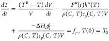13a

13b

13c

13d

where ϕ_c(C,T) = 3ρ_cVk_vM₂G(C,T), M₂ = ∫₀^∞n(L)L²dL.

Population Balance Equation PBE

14

Note that the physical properties (h^w, ρ, Cp) of the liquid and vapor phases are calculated by means of polynomial functions which are nonlinear in the temperature and in the concentration. Thus, the model of the process (eqs 13–14) is constituted by a system of partial-integro differential equations and algebraical equations which are nonlinear and coupled. The system (eqs 13–14) is input-to-state (SI)²⁵ stable.

Crystallization Kinetics

The model accounts for the following crystallization kinetics. The size-independent power law kinetics for crystal growth G (eq 15) is widely used in crystallization modeling^13,22 because of its simplicity. The secondary nucleation B₀ (eq 16) is modeled through the Evans kinetics³³ when only crystal-impeller collisions are considered.

15

16

In eq 15 and eq 16, k_g and k_ci are kinetics parameters. In eq 16, N_Q, N_P, and ε are impeller parameters. One can refer to the notation section for their meaning.

The birth B_A and death D_A functions due to agglomeration phenomena are modeled according to ref (11), as shown in eq 17 and eq 18.

17

18

Note that the modeling of the agglomeration phenomena is a source of important nonlinearities for the system. The agglomeration Kernel β defines the probability of agglomeration between crystals, and it is considered size independent and calculated according to the empirical expression (eq 19).

19

In eq 19, a is a kinetic parameter. The values of the kinetic and impeller parameters are reported in Table 1. The kinetic parameters of Case 1 are taken from Porru and Özkan.²⁹ Case 2 has supersaturation orders for growth (g_g) and nucleation (g_n) greater than one which are representative of a class of crystallization systems of pharmaceutical interest.³⁴⁻³⁷

Table 1. Kinetic and Impeller Parameters.

Parameter	Case 1	Case 2
kg	4.64 × 10–5	4.64 × 10–5	m/s
kci	exp(12.54)	exp(12.54)	#/m3 s
gg	1	1.1	–
gn	1	2	–
Lmin	100	100	μm
a	3.016 × 10–12	3.016 × 10–12	–
NQ	1.6	1.6	–
NP	2	2	–
ε	2.1	2.1	m2/s3

Solution of PBE through MOC

The PBE solution is obtained with the method of characteristics³⁸ (MOC). A detailed discussion of the numerical scheme adopted can be found in Porru and Özkan.²⁹

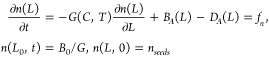
After application of the MOC and discretization along the length domain, the PBE (eq 14) is transformed in the system of ODEs

20

Note the following:

• (i)B_A(L_i) and D_A(L_i) are the discretized versions of eq 17 and eq 18.
• (ii)The number of ODEs constituting the system (eqs 20) increases with time by virtue of the movement of the mesh grid due to growth and the necessity to generate a new cells of length L₀ to allocate new nuclei.¹⁷
• (iii)On the basis of this, in system eqs 20, i = 1,...,N_c(t), and N_c is the number of the grid points in the mesh grid.
• (iv)The PBE (eq 14) (and its discretized version (eqs 20)) is coupled with the material and energy balances for the liquid phase through the process variables C and T needed to compute the crystallization kinetics (eqs 15–19), and M₂.

A numerical scheme for the solution of the system (eqs 20) can be found in the Appendix. The discretized PBE model (eqs 20) together with the macroscopic balance equations (eqs 13) are used for observability analysis and to generate the measurements of the secondary variables (temperature and solid fraction) that will be used to estimate concentration and CSD.

Compact Notation

The system of equations (eq 13 and 20) is here rewritten in compact notation:

where

Simulation of the Model

Physical properties and kinetics parameters are set to return a behavior of the CSD representative of industrial operations. The flow rate of vapor F^w is an input of the system chosen to guarantee a low and almost constant supersaturation level over the batch run. It is assumed to be given.

The behavior of the crystallization system is simulated in MATLAB R2016a and a computer with Intel(R) Core (TM)2 Quad CPU 2.83 GHz. The ODEs (eqs 13) are solved with ODE45 with a 60 s sampling time. At the end of this time interval, the growth, nucleation, and agglomeration rates are calculated and used to upgrade the CSD dynamics by applying the Euler algorithm to eqs 20. The nuclei are accommodated in the length class L₀ = 0.1 μm.

For the cases at hand, the seeds are lognormally distributed with mean μ_seeds = 74 μm and spread σ_seeds = 1.2. The initial mesh grid is uniformly distributed and consists of 300 lengths with length interval of 2 μm.

A predefined vapor profile is applied for 6720 s (112 min) and generates monotonically decreasing temperature, concentration, and volume profiles. The initial and final values of the vapor flow are 0.005 and 0.001 kg/s, respectively. The flow is maximum (about 0.09 kg/s) around 1000 s. The temperature variation is 22.5 K between its initial and final value. The variation between the initial and final concentration is 141.9 kg/m³. The volume variation is 0.3 m³. For the parameters of Case 1 in Table 1, Figure 1 shows the CSD at time zero (seeds) at one forth of the batch run and at its end. From Figure 1, one can notice three modes in the volume fraction v (v_i = n_ik_vL_i³) that can be associated with (i) nucleation and agglomeration of the nuclei, (ii) growth of seeds, and (iii) growth and agglomeration of the initial seeds.

Figure 1.

CSD in terms of volume fraction v at the beginning of the batch (seed), after 28 min and at the end of the batch run.

The simulation of 6720 s of a batch run takes approximatively 62 s for both cases in Table 1. According to Huisman,³⁹ a nonlinear model can be used for online applications if it is faster than the real process by a factor of 100. Hence, the proposed model can be employed as an estimation model.

3.2. Structure Design for Flash Cooling Crystallization

The estimation problem for the batch flash cooling crystallization consists of providing a proper estimation of the solute concentration C and the CSD (defined by the pair L_i - n_i, i = 1,...,N_C) by means of secondary measurements, namely, temperature T and solid fraction ϵ_S. The chosen estimation algorithm is the GE (eqs 10) in the understanding that the estimation performance relies on the choice of a proper estimation structure rather than the estimation algorithm.

The analysis is done by means of RE-estimability concepts previously described. One measurement at a time is considered.

RE-Estimability with Temperature Measurements

In the case of temperature measurements, the output map assumes the linear form: y₁ = C₁x, C₁ = [1,0,0,...,0]^T. The computation of the corresponding sequence N – 1 of repeated Lie derivatives which defines the nonlinear map ϕ_T(x,U(t)) (eq 21) cannot be performed in practice because of the high dimensionality of the system; however, from the analysis of the first two ones, one can draw conclusive information:

21

Due to the fact that the nonlinear map ϕ_T(x,U(t)) is a function of only T, C, and V, the corresponding surface Ξ_T(x,U(t)) = ∂ϕ_T(x,U(t))/∂x has rank 3, and it is CSD (L_i–n_i, i = 1, ..., N_c) independent, meaning that the system is not RE-observable. However, the subset of ϕ_T defined as ϕ_ι,T(x,U(t)) = [h₁,L_fh₁,L_f²h₁]^T with κ_ι,T = 3 generates a Ξ_ι,T satisfying the detectability conditions (eqs 6) for the distinguishable states x_ι,T = [T,C,V]^T. This in turn means the following:

• (i)The subset of state T, C, and V is distinguishable with temperature measurements.
• (ii)The particle size distribution L_i – n_i, i = 1,...,N_c is not distinguishable with temperature measurements.

Moreover, from the first-order Lie derivative L_fh₁ = f_t (eq 13a), one can note that the solute concentration C is undistinguishable with temperature measurements when the heat of crystallization ΔH_c = 0 because the variation of the physical properties c_p and ρ is weak during a batch run or when the growth rate G → 0. The latter is verified for supersaturation C – C_sat → 0, which normally happens at the end of the batch run. In these cases, the set of distinguishable states reduces to x_ι,T = [T,V]^T.

RE-Estimability with Solid Fraction Measurements

Solid fraction measurements can be recovered from density measurement instruments that determine differential pressure measurements. Such measurements can be successfully taken by locating the instrument at two different points beneath the liquid surface or in the circulation system far enough from turbulence.^40,41 The turbulence causes noise which can be removed with a suitable electrical dampening.⁴⁰ These types of measurements have been used for parameter estimation in a 75 L DT crystallizer.⁴² Examples of reliable solid fraction measurements have been obtained from an industrial batch crystallizer of 1100 L capacity by Kalbasenka⁴¹ and used for parameter estimation and optimization purposes.

In the case of solid fraction measurements, the output map is y₂ = h₂(V,C) = M/(Vρ_c). The corresponding repeated Lie derivatives sequence in the ϕ_ϵS matrix is

22

which is difficult to compute in practice for high-dimensional systems. However, one can note from the computation of the first two Lie derivatives that ϕ_ϵS only depends on T, C, and V. Accordingly, the corresponding surface Ξ_ϵS(x,U(t)) = ∂ϕ_ϵS(x,U(t))/∂x has rank 3, and it is CSD (L_i – n_i, i = 1,...,N_c) independent, meaning that the CSD is undistinghuishable with solid fraction measurements as well, and the system is not RE-observable. However, the subset of ϕ_ϵS(x,U(t)) defined as ϕ_ι,ϵS(x,U(t)) = [h₂,L_fh₂,L_f²h₂]^T with κ_ι,ϵS = 3 generates a Ξ_ι,ϵS(x,U(t)) satisfying the detectability conditions (eqs 6) for the distinguishable states x_ι,ϵS = [T, C, V]^T. This in turn means that the subset of state T, C, and V is distinguishable with solid fraction measurements, while the CSD size distribution is not.

Moreover, from the computation of the first-order Lie derivative

23

one can notice that in practice the concentration is distinguishable only if the second moment M₂ of the CSD and the growth rate G are large enough. Considering that at the beginning of the batch the solid phase is in negligible quantity and that at the end of the batch the supersaturation is almost all consumed, there is a lack of estimability of the concentration at the beginning and end of the batch run, when M₂ ≃ 0 and G ≃ 0.

Estimator Structure

The outcome the estimability study shows that the solute concentration is distinguishable through temperature and solid fraction measurements, while the CSD is undistinguishable. The obtained results represent the starting point for the design of the structure of the estimator. Even if the system is not observable, it is detectable because the dynamics of the undistinguishable states are stable according to the definition of stability for batch processes given by Srinivasan and BonvinSrin.⁴³ In the light of the estimation objective (i.e., estimation of the primary variables: solute concentration and CSD), the performed estimability analysis of the crystallization system suggests the following:

• (i)Due to the undistinghuishability of CSD, the estimation model has to be detailed in the description of the CSD dynamics, that is to say that the accuracy of the prediction of the CSD behavior relies on the goodness of the discretized PBE. In this case, it is appropriate to use the rigorous model of the crystallization (eqs 13–20) as estimation model since it is accurate and suitable for online use (i.e., it can be simulated 100 times faster than the real process³⁹).
• (ii)Considering that the estimators with detectability indexes larger than two generally leads to an ill-conditioned estimation, one should choose up to a maximum of two innovated states per measurements. Among the distinguishable states, the choice of the innovated states should guarantee a good trade off between innovation of the states describing the dynamics of the primary variables and innovation of the states whose changes much affect the measured outputs of the system. For this reason, it is reasonable choosing to innovate (a) temperature and concentration by means of temperature measurements and (b) mass of crystal and concentration by means of the solid fraction measurements.

As it is demonstrated in the following sections, this structure guarantees a good estimation of the concentration under measurement noises and model-plant mismatch and good estimation of the CSD if its estimation model and the plant are made to start sufficiently close.

4. Results

4.1. Concentration and CSD Estimator

From the discussion in the previous paragraphs, the passive estimator (eqs 24) is proposed. The estimation has innovation of temperature and concentration dynamics (and concentration and solid mass dynamics) by means of temperature (and solid fraction) measurements. The measurements are processed with a GE with a proportional innovation mechanism. The CSD is estimated in an open loop mode by means of the discretized PBE.

24a

24b

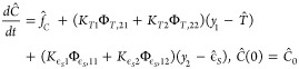24c

24d

24e

24f

where K_T1 and K_T2 (and K_ϵ1 and K_ϵ2) are the proportional gains related with the innovation through temperature (and solid fraction) measurements. Φ_T,ij are the elements of the (2 × 2) matrix Φ_T which is the inverse of O_ιT(x,u(t))

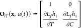25

with L_fh₁ = f_T (eq 21). The elements of the second row of O_ιT(x, u(t)) are

with temperature and concentration dependency of the density ρ and specific heat c_p being neglected.

Φ_ϵS,ij are the elements of the (2 × 2) matrix Φ_ϵS which is the inverse of O_ιϵS

26

with L_fh₂ reported in eq 23. The elements of the second row of O_ιϵS(x, u(t)) are

with concentration dependency of the density ρ being neglected.

It is worth noticing that Φ_T and Φ_ϵS are time-dependent matrices as well as O_ιT and O_ιϵS since the latter are functions of the input u(t). From this point of view, the realization of the GE for batch systems can be seen as an estimator with adaptive gains K_TΦ_T(t) and K_ϵΦ_ϵS(t). Furthermore, O_ιT and O_ιϵS are input derivative-free, and the computation of these matrices is not challenging, both in the cases of g_g ≠ 1 and g_g = 1 since C_sat is a polynomial function of T and hence analytically differentiable in T.

4.2. Performance Evaluation of the Estimator

Industrial batch crystallization processes are prone to operate under uncertainties, which are due to measurement deficiency, uncertain initial conditions, and uncertainties associated with the kinetics parameters. To this end, the proposed estimator is tested under the following scenarios: (i) uncertain initial concentration, (ii) uncertain heat of crystallization, (iii) uncertain initial distribution of seeds, (iv) uncertain kinetic parameters, and (v) literature-based¹⁸ uncertain scenario.

The model with parameters of Case 1 in Table 1(29) are considered for scenarios i, ii, and iii. Estimation performances with Case 1’s and Case 2’s parameters are tested for scenario iv. Estimation performance with Case 2’s parameters is tested for the scenario v. The temperature and solid fraction measurements are obtained by simulating the model without any uncertainty under a predefined vapor flow (input) trajectory and a sampling time of 1 min. Then, secondary variables and input are corrupted with a 65 dB white noise. For the parameters of Case 1, the measurements of the secondary variables for state estimation are depicted in Figure 2. With parameters of Case 2, the trajectories are similar and hence not presented. The estimator is tuned according to the guidelines (eq 11) with observer frequency ω_o = 20 ω_c and damping factor ξ = 1. The inverse of the batch run time is taken in place of the characteristic frequency ω_c of the crystallization. The proposed estimator is programmed in MATLAB R2016a, and it takes approximately 62 s to simulate 6720 s of real process in a computer with Intel (R) Core (TM)2 Quad CPU 2.83 GHz.

Figure 2.

Measurements of the secondary variables: (a) temperature and (b) solid fraction.

Note that, for better readability, CSD results are given in terms of volume fraction v rather than number density function n. Between the two variables, the relation v_i = n_ik_vL_i³ holds. Information about the median size of the crystals in terms of D50 is also given (D50 is the 50th percentile of the cumulative of the CSD expressed in terms of volume fraction v).

Uncertain Initial Concentration

In this test, the estimator is run with a +10% mismatch in C₀ (eq 24c) with respect to the reference model. Under this scenario, the estimation model without any innovation manifests a consistent bias in the prediction of both the concentration (Figure 3a) and the CSD (Figure 3b) and its attributes (D50, Figure 3c). On the other hand, if the temperature and solid fraction measurements are used the trajectory of the concentration (Figure 3d), the CSD (Figure 3e) and the D50 (Figure 3f) converges to the reference trajectory. The convergence time depends on the low distinguishability of the concentration at the beginning of the batch run which is associated with the small amount of crystal surface present, as found in Section 3.2. Accordingly, the convergence rate cannot be improved by tuning. The reference system has parameters according to Case 1 in Table 1.

Figure 3.

Estimation of the model without any innovation (top) and of the proposed estimator (bottom) of concentration (a,d), CSD at every 10 min of operation (b,e), and D50 (c,f), under 10% of uncertainty in the initial solute concentration.

Uncertain Heat of Crystallization

In this scenario, a high level of uncertainty is assumed for the heat of crystallization, and in the estimation model, this parameter is taken at 1/10 of the reference value. Under this severe test, one can note that the estimation model without any innovation predicts a much higher consumption of solute (Figure 4a), while the estimator is able to reconstruct the concentration profile with high accuracy (Figure 4d). On the other hand, the convergence of the concentration estimation penalizes the transient of the estimation of the CSD (Figure 4e) and its attributes (D50, (Figure 4f)), leading to offsets. The reference system has parameters according to Case 1 in Table 1.

Figure 4.

Estimation of the model without any innovation (top) and of the proposed estimator (bottom) of concentration (a,d), CSD at every 10 min of operation (b,e), and D50 (c,f), under high uncertainty in the heat of crystallization.

Uncertain Median of Initial Seeds

This uncertain scenario corresponds to an error of the +10% in the initial mean of the seeds. The performance of the estimation model without any innovation and the ones of the estimator with secondary measurements are presented in Figure 5. Both the model (Figure 5a) and the estimator (Figure 5d) give the correct prediction of the concentration and an estimation of the CSD with limited offsets. However, the estimator gives a slightly better estimation of the shape of the CSD (Figure 5e) and its D50 (Figure 5f). The reference system has parameters according to Case 1 in Table 1.

Figure 5.

Estimation of the model without any innovation (top) and of the proposed estimator (bottom) of concentration (a,d), CSD at every 10 min of operation (b,e), and D50 (c,f), under 10% of uncertainty in the median size of the seeds distribution.

Uncertain Kinetics Parameters

Under this scenario, a mismatch between the kinetics parameters of the estimation model and the reference model is assumed. The performance is tested against a reference system with parameters of Case 1 and Case 2 in Table 1.

For the system with parameters of Case 1, we assume that the mismatch between the reference model and the estimation model amounts to a +10% error in the growth and nucleation rate constant (k_g and k_ci) and in the agglomeration parameter a. The simulation results are shown in Figure 6. Under this scenario, the concentration of the solute is predicted with good performance, both with the model without innovation (Figure 6a) and the estimator (Figure 6d). As expected from the estimability analysis, the estimator driven by secondary measurements is not able to deal with errors in the population balance equation (PBE) leading to an estimation of the CSD (Figure 6e) which is comparable with the one obtained from the model without any innovation (Figure 6b). This is because the CSD is indistinguishable with these measurements, or in other words, variations in the evolution of the CSD are not captured by means of temperature and solid fraction measurements. This confirms that the estimation of undistinguishable dynamics relies on the accuracy of the estimation model, as stated in the estimator structure design section.

Figure 6.

Estimation of the model without any innovation (top) and of the proposed estimator (bottom) of concentration (a,d), CSD at every 10 min of operation (b,e), and D50 (c,f), under 10% of uncertainty in the kinetics parameters k_g, k_ci, and a.

To the best of the authors’ knowledge, the majority of the papers in the area of modeling of crystallization processes do not give clear information about the uncertainty attached to the parameters. In some cases, 95% confidence limits have been reported. According to Qiu and Rasmuson,⁴⁴ an appropriate choice of the estimation technique, the objective function, and the experiment operating conditions may limit the uncertainty in the parameters as follows:

• (S.a)Qiu and Rasmuson⁴⁴ reported 15–20% for the nucleation rate constant, 1.6–3.5% for the growth rate constant, 10% for the supersaturation order of the growth rate, and 2.6% for the supersaturation order of the nucleation rate.
• (S.b)By means of data discrimination, the mismatch in the nucleation parameters can be further reduced. In this case Qiu and Rasmuson⁴⁴ reported mismatches of 10% for the nucleation rate constant, 7% for the growth rate constant, 6% for the supersaturation order of the growth rate, and 0% for the supersaturation order of the nucleation rate.

A simulation has been carried out to test the performance of the estimator under the parametric plant-model mismatch (S. a), and an initial concentration mismatch of +5%. Table 2 compares the values of the parameters in the reference model (Case 2 in Table 1) and the estimation model under this uncertain scenario. The performance of the estimator is satisfactory (Figure 7).

Table 2. Parameters Information for Case 2.

Parameter	Case 2: Reference Model	Estimation model	Units	Mismatch
kg	4.64 × 10–5	4.80 × 10–5	m/s	+3.5%
kci	exp(12.54)	exp(12.7226)	#/m3s	+20%
gg	1.1	1.21	–	+10%
gn	2	2.052	–	+2.6%
a	3.016 × 10–12	3.122 × 10–12	–	+3.5%

Figure 7.

Performance of the estimator under the uncertain scenario (S.a)⁴⁴ (Table 2) and an initial concentration mismatch of +5%: concentration (a), CSD at every 10 min of operation (b), and D50 (c).

Literature-Based¹⁸ Uncertain Scenario

This scenario considers parametric plant-model mismatches and uncertain initial conditions at the same time: (i) Parametric plant-model mismatches: + 15% error in kinetic parameters¹⁸ and (ii) Uncertain initial conditions: + 2% error in the initial solute concentration, and +5% error in the mean of the initial CSD.¹⁸

The estimator based on the system with parameters of the Case 2 in Table 1 is tested under this uncertain scenario. Simulation results are depicted in Figure 8. The concentration is perfectly and quickly recovered by the estimator, and the estimation of the CSD is satisfactory, even if the CSD dynamics is not distinguishable with the measurements of temperature and solid fraction. The shape of the CSD is very well preserved, and the mismatch between the reference D50 and the estimated one is only ≈6.5%.

Figure 8.

Performance of the estimator under a literature-based¹⁸ uncertain scenario: concentration (a), CSD at every 10 min of operation (b), and D50 (c).

4.3. Remarks

In this section, the performance of the designed estimator are tested under uncertain scenarios. The estimation performance is in line with the expectation in light of the performed estimability analysis. In particular, the estimation of the concentration profile is always good. The estimation of the CSD is acceptable provided that the estimation model is accurate enough. In fact, a good estimation of the CSD relies on a detailed description of the crystallization phenomena in place (growth, nucleation, and agglomeration) and a confident parameter estimation, which is in agreement with our structure selection guidelines.

5. Conclusions

In this work, a concentration and crystal size distribution (CSD) estimator driven by secondary variables (temperature and solid fraction) measurements has been developed and tested for a crystallization system accounting for growth, secondary nucleation, and agglomeration. The estimation problem is cast as an estimation structure problem in the understanding that the estimation performance relies on an appropriate structure selection rather than the chosen estimation algorithm. The estimation structure design has been performed based on guidelines driven from RE-estimability arguments. For the case under study, RE-estimability analysis mostly suggests to use a detail estimation model to provide the best prediction possible of the undistinguishable CSD dynamics and a passive innovation scheme with temperature, concentration, and mass of crystals as innovated states. The used estimation algorithm is the GE with proportional innovation which offers simplicity of tuning and implementation. Estimation testing through simulations have confirmed our expectations: the performance of the designed estimator is always good with respect to the concentration estimation and acceptable for the CSD provided that an accurate rigorous model is available.

Glossary

Nomenclature

a

Agglomeration parameter

B_A

Birth function due to agglomeration [#/s μm m³]

B₀

Nucleation rate for primary and secondary nucleation [#/s m³]

C

Solute concentration [kg/m³]

c_p

Specific heat of the mixture [J/kgK]

C_sat

Solute concentration at saturation [kg/m³]

D_A

Death function due to agglomeration [#/s μm m³]

G

Crystal growth rate [m/s]

g_g

Supersaturation order in the growth rate law [−]

g_n

Supersaturation order in the nucleation law [−]

k_g

Growth rate constant [m/s]

k_ci

Nucleation rate constant [#/m³ s]

k_v

Volumetric shape factor [−]

L

Internal coordinate crystal length [m]

L₀

Characteristic length of crystal nuclei [m]

L_min

Crystal length above which crystals undergo attrition [m]

M

Mass of crystals [kg]

M₂

Second moment of the CSD, proportional to the total crystal surface [# m²/m³]

n

Number density function [#/m³ μm]

n_seeds

Number density function of the seeds [#/m³ μm]

N_Q

Impeller flow number [−]

N_P

Impeller power number [−]

T

Temperature of the system [K]

T^R

Reference temperature [K]

t

Time [s]

V

Volume [m³]

v

Volume fraction [m³/μm m³]

F^w

Mass flow of the vapor [kg/s]

h^w

Enthalpy of the vapor [J/kg]

ΔH_C

Heat of crystallization [J/kg]

β

Agglomeration kernel [−]

ϵ_S

Solid fraction [−]

ε

Specific power input [m²/s³]

ρ

Density of the mixture [kg/m³]

ρ_c

Density of the solid phase [kg/m³]

ϕ_c

Crystal production term due to crystal growth [kg/s]

Appendix

Numerical Solution Scheme for Population Balance Equation with Simultaneous Growth, Nucleation, and Agglomeration

In this Appendix, the numerical scheme adopted for the simulation of the CSD dynamics (eqs 20) is presented.

Let us define Λ = [L₀,L₁,L₂,...,L_max]^T as the vector of dimension dim(Λ) = γ containing the length classes obtained by discretizing the internal coordinate L. Let N = [n(L₀), n(L₁), n(L₂), ..., n(L_max)]^T (or in short N = [n₀,n₁,n₂,...,n_max]^T) be the vector of number densities associated with each length class having dim(N) = dim(Λ) = γ. The crystal size distribution if univocally identified by the pair [Λ,N].

Let (t_fin – t_in) be the sampling time of the numerical scheme and N_samp be the number of iteration needed to simulate the batch time. The dynamics of the CSD (eqs 20) can be simulated by means of the following numerical scheme:

27a

27b

27c

27d

27e

27f

27g

27h

In eqs 27, G_in denotes the growth rate at the time t_in. B_A(L_i,t_in) (or D_A(L_i,t_in)) denotes the birth (or death) rate of crystals in the length class L_i at the time t_in. n_i,tfin^* is the number of particle per unit volume due to the nucleation and growth phenomena according to

28a

28b

where B_0,in denotes the birth rate at time t_in.

∀L_i ∈ Λ:

• 1.
  The evaluation of the birth rate

  29

  involves the computation of the elements Λ_i,j^* of the vector Λ_i

  

  

  being γ_i^* the dimension of the subset of crystal classes

  30

  31
• 2.Evaluate the number density n(Λ_i,j^*) corresponding to each crystal length Λ_i,j by extrapolation, involving the two adjacent length classes L_k, L_k+1 such that L_k < (L_i³ – L_j)^1/3 < L_k+1 and the corresponding number densities n(L_k) and n(L_k+1).
• 3.
  Evaluate the elements F_i,j of the vector F_i = [F_i,1,...,F_i,γi^*]^T according to

  

  The integral term I_B(L_i) in eq 29

  

  is evaluated by computing the area under the curve defined by the matrix of points [Λ_i^–, F_i]^T by means of a trapezoidal rule.
• 4.
  The birth rate by agglomeration

  32

  can be evaluated by means of the approximation of the integral

  33

  A detailed analysis of the performance of this algorithm can be found in the paper by Porru and Özkan.²⁹

The authors declare no competing financial interest.

References

- Eek R. A.; Bosgra O. H. Controllability of particulate processes in relation to the sensor characteristics. Powder Technol. 2000, 108, 137–146. 10.1016/S0032-5910(99)00211-9. [DOI] [Google Scholar]
- Simon L. L.; et al. Assessment of recent process analytical technology (PAT) trends: a multiauthor review. Org. Process Res. Dev. 2015, 19, 3–62. 10.1021/op500261y. [DOI] [Google Scholar]
- Frau A.; Baratti R.; Alvarez J. Composition estimation of a six-component distillation column with temperature measurements. IFAC Proceedings Volumes 2009, 42, 429–434. 10.3182/20090712-4-TR-2008.00068. [DOI] [Google Scholar]
- Frau A.Composition Control and Estimation with Temperature Measurement for Multicomponent Distillation Columns. Ph.D. Thesis, Universita’ degli Studi di Cagliari, 2011. [Google Scholar]
- Fernandez C.; Alvarez J.; Baratti R.; Frau A. Estimation structure design for staged systems. J. Process Control 2012, 22, 2038–2056. 10.1016/j.jprocont.2012.07.012. [DOI] [Google Scholar]
- Porru M.; Alvarez J.; Baratti R. A distillate composition estimator for an industrial multicomponent IC4-NC4 splitter with experimental temperature measurements. IFAC Proceedings Volumes 2013, 46, 391–396. 10.3182/20131218-3-IN-2045.00028. [DOI] [Google Scholar]
- Porru M.Quality regulation and energy saving through control and monitoring techniques for industrial multicomponent distillation columns. Ph.D Thesis, Universita’ degli Studi di Cagliari, 2015. [Google Scholar]
- Hulburt H. M.; Katz S. Some problems in particle technology: A statistical mechanical formulation. Chem. Eng. Sci. 1964, 19, 555–574. 10.1016/0009-2509(64)85047-8. [DOI] [Google Scholar]
- Randolph A. D.; Larson M. A.. Theory of Particulate Processes, Analysis and Techniques of Continuous Crystallization; Academic Press, 1971. [Google Scholar]
- Ramkrishna D. The status of population balances. Rev. Chem. Eng. 1985, 3, 49–95. 10.1515/REVCE.1985.3.1.49. [DOI] [Google Scholar]
- Hounslow M.; Ryall R.; Marshall V. A discretized population balance for nucleation, growth, and aggregation. AIChE J. 1988, 34, 1821–1832. 10.1002/aic.690341108. [DOI] [Google Scholar]
- Cogoni G.; Frawley P. Particle size distribution reconstruction using a finite number of its moments through artificial neural networks: A practical application. Cryst. Growth Des. 2015, 15, 239–246. 10.1021/cg501288z. [DOI] [Google Scholar]
- Mesbah A.; Huesman A. E.; Kramer H. J.; Van den Hof P. M. A comparison of nonlinear observers for output feedback model-based control of seeded batch crystallization processes. J. Process Control 2011, 21, 652–666. 10.1016/j.jprocont.2010.11.013. [DOI] [Google Scholar]
- Shi D.; Mhaskar P.; El-Farra N. H.; Christofides P. D. Predictive control of crystal size distribution in protein crystallization. Nanotechnology 2005, 16, S562–S574. 10.1088/0957-4484/16/7/034. [DOI] [PubMed] [Google Scholar]
- Nagy Z. K.; Braatz R. D. Robust nonlinear model predictive control of batch processes. AIChE J. 2003, 49, 1776–1786. 10.1002/aic.690490715. [DOI] [Google Scholar]
- Baterham R.; Hall J.; Barton G.. Pelletizing Kinetics and Simulation of Full Scale Balling Circuits. In Proceedings of the Third International Symposium on Agglomeration, Nurnberg, West Germany, 1981; pp A136–A144.
- Mesbah A.; Kramer H. J.; Huesman A. E.; Van den Hof P. M. A control oriented study on the numerical solution of the population balance equation for crystallization processes. Chem. Eng. Sci. 2009, 64, 4262–4277. 10.1016/j.ces.2009.06.060. [DOI] [Google Scholar]
- Mesbah A.; Nagy Z. K.; Huesman A. E.; Kramer H. J.; Van den Hof P. M. Nonlinear model-based control of a semi-industrial batch crystallizer using a population balance modeling framework. IEEE Transactions on Control Systems Technology 2012, 20, 1188–1201. 10.1109/TCST.2011.2160945. [DOI] [Google Scholar]
- Bakir T.; Othman S.; Fevotte G.; Hammouri H. Nonlinear observer of crystal-size distribution during batch crystallization. AIChE J. 2006, 52, 2188–2197. 10.1002/aic.10820. [DOI] [Google Scholar]
- Cogoni G.; Tronci S.; Mistretta G.; Baratti R.; Romagnoli J. A. Stochastic approach for the prediction of PSD in nonisothermal antisolvent crystallization processes. AIChE J. 2013, 59, 2843–2851. 10.1002/aic.14089. [DOI] [Google Scholar]
- Baratti R.; Tronci S.; Romagnoli J. A. A generalized stochastic modelling approach for crystal size distribution in antisolvent crystallization operations. AIChE J. 2017, 63, 551–559. 10.1002/aic.15372. [DOI] [Google Scholar]
- Abbas A.; Romagnoli J. A. Multiscale modeling, simulation and validation of batch cooling crystallization. Sep. Purif. Technol. 2007, 53, 153–163. 10.1016/j.seppur.2006.06.027. [DOI] [Google Scholar]
- Zhang B.; Willis R.; Romagnoli J.; Fois C.; Tronci S.; Baratti R. Image-based multiresolution-ann approach for online particle size characterization. Ind. Eng. Chem. Res. 2014, 53, 7008–7018. 10.1021/ie4019098. [DOI] [Google Scholar]
- Porru M.; Özkan L. Systematic observability and detectablity analysis of industrial batch crystallizers. IFAC-PapersOnLine 2016, 49, 496–501. 10.1016/j.ifacol.2016.07.391. [DOI] [Google Scholar]
- Álvarez J.; Fernández C. Geometric estimation of nonlinear process systems. J. Process Control 2009, 19, 247–260. 10.1016/j.jprocont.2008.04.017. [DOI] [Google Scholar]
- Alhoniemi E.; Hollmén J.; Simula O.; Vesanto J. Process monitoring and modeling using the self-organizing map. Integrated Computer Aided Engineering 1999, 6, 3–14. [Google Scholar]
- Corona F.; Mulas M.; Baratti R.; Romagnoli J. A. Data-derived analysis and inference for an industrial deethanizer. Ind. Eng. Chem. Res. 2012, 51, 13732–13742. 10.1021/ie202854b. [DOI] [Google Scholar]
- Alvarez J. Nonlinear state estimation with robust convergence. J. Process Control 2000, 10, 59–71. 10.1016/S0959-1524(99)00018-9. [DOI] [Google Scholar]
- Porru M.; Özkan L. Monitoring of batch industrial crystallization with growth, nucleation and agglomeration. Part 1: modelling with method of characteristics. Ind. Eng. Chem. Res. 2017, 56, 5980–5992. 10.1021/acs.iecr.7b00240. [DOI] [PMC free article] [PubMed] [Google Scholar]
- Dochain D. State and parameter estimation in chemical and biochemical processes: a tutorial. J. Process Control 2003, 13, 801–818. 10.1016/S0959-1524(03)00026-X. [DOI] [Google Scholar]
- Tronci S.; Bezzo F.; Barolo M.; Baratti R. Geometric observer for a distillation column: development and experimental testing. Ind. Eng. Chem. Res. 2005, 44, 9884–9893. 10.1021/ie048751n. [DOI] [Google Scholar]
- Alvarez J.; Lopez T. Robust dynamic state estimation of nonlinear plants. AIChE J. 1999, 45, 107–123. 10.1002/aic.690450110. [DOI] [Google Scholar]
- Evans T.; Sarofim A.; Margolis G. Models of secondary nucleation attributable to crystal-crystallizer and crystal-crystal collisions. AIChE J. 1974, 20, 959–966. 10.1002/aic.690200517. [DOI] [Google Scholar]
- Cogoni G.; de Souza B.; Frawley P. J. Particle Size Distribution and yield control in continuous Plug Flow Crystallizers with recycle. Chem. Eng. Sci. 2015, 138, 592–599. 10.1016/j.ces.2015.08.041. [DOI] [Google Scholar]
- Power G.; Hou G.; Kamaraju V. K.; Morris G.; Zhao Y.; Glennon B. Design and optimization of a multistage continuous cooling mixed suspension, mixed product removal crystallizer. Chem. Eng. Sci. 2015, 133, 125–139. 10.1016/j.ces.2015.02.014. [DOI] [Google Scholar]
- Shi D.; Mhaskar P.; El-Farra N. H.; Christofides P. D. Predictive control of crystal size distribution in protein crystallization. Nanotechnology 2005, 16, S562. 10.1088/0957-4484/16/7/034. [DOI] [PubMed] [Google Scholar]
- Mitchell N. A.; Frawley P. J.; Ó'Ciardhá C. T. Nucleation kinetics of paracetamol-ethanol solutions from induction time experiments using Lasentec FBRM®. J. Cryst. Growth 2011, 321, 91–99. 10.1016/j.jcrysgro.2011.02.027. [DOI] [Google Scholar]
- Kumar S.; Ramkrishna D. On the solution of population balance equations by discretization - III. Nucleation, growth and aggregation of particles. Chem. Eng. Sci. 1997, 52, 4659–4679. 10.1016/S0009-2509(97)00307-2. [DOI] [Google Scholar]
- Huisman L.Control of Glass Melting Processes Based on Reduced CFD Models. Ph.D. Thesis, Technische Universiteit Eindhoven, 2005. [Google Scholar]
- Myerson A.Handbook of Industrial Crystallization; Butterworth-Heinemann, 2002. [Google Scholar]
- Kalbasenka A. N.Model-Based Control of Industrial Batch Crystallizers. Experiments on Enhanced Controllability by Seeding Actuation. Ph.D. Thesis, TU Delft, Delft University of Technology, 2009. [Google Scholar]
- Kalbasenka A.; Huesman A.; Kramer H. Modeling batch crystallization processes: Assumption verification and improvement of the parameter estimation quality through empirical experiment design. Chem. Eng. Sci. 2011, 66, 4867–4877. 10.1016/j.ces.2011.06.049. [DOI] [Google Scholar]
- Srinivasan B.; Bonvin D. Controllability and stability of repetitive batch processes. J. Process Control 2007, 17, 285–295. 10.1016/j.jprocont.2006.10.009. [DOI] [Google Scholar]
- Qiu Y.; Rasmuson Å. C. Estimation of crystallization kinetics from batch cooling experiments. AIChE J. 1994, 40, 799–812. 10.1002/aic.690400507. [DOI] [Google Scholar]