Demonstration of Multi- and Single-Reader Sample Size Program for Diagnostic Studies software

Abstract

The recently released software Multi- and Single-Reader Sample Size Sample Size Program for Diagnostic Studies, written by Kevin Schartz and Stephen Hillis, performs sample size computations for diagnostic reader-performance studies. The program computes the sample size needed to detect a specified difference in a reader performance measure between two modalities, when using the analysis methods initially proposed by Dorfman, Berbaum, and Metz (DBM) and Obuchowski and Rockette (OR), and later unified and improved by Hillis and colleagues. A commonly used reader performance measure is the area under the receiver-operating-characteristic curve.

The program can be used with typical common reader-performance measures which can be estimated parametrically or nonparametrically. The program has an easy-to-use step-by-step intuitive interface that walks the user through the entry of the needed information. Features of the software include the following: (1) choice of several study designs; (2) choice of inputs obtained from either OR or DBM analyses; (3) choice of three different inference situations: both readers and cases random, readers fixed and cases random, and readers random and cases fixed; (4) choice of two types of hypotheses: equivalence or noninferiority; (6) choice of two output formats: power for specified case and reader sample sizes, or a listing of case-reader combinations that provide a specified power; (7) choice of single or multi-reader analyses; and (8) functionality in Windows, Mac OS, and Linux.

1. INTRODUCTION

In this paper we discuss the recently released software Multi- and Single-Reader Sample Size Sample Size Program for Diagnostic Studies, written by Kevin S. Schartz and Stephen L. Hillis. This software performs sample size and power computations for sizing future diagnostic reader-performance studies. Such studies are commonly used in radiology, where radiologists evaluate images resulting from an imaging modality with respect to confidence of disease. The program can be freely downloaded from http://perception.radiology.uiowa.edu/.

The program computes the sample size needed to detect a specified difference in a reader performance measure between two modalities when using the analysis methods initially proposed by Dorfman, Berbaum, and Metz (DBM)^1–2 and Obuchowski and Rockette (OR)³ and later unified, improved, and generalized by Hillis and colleagues^4–7. We refer to the improved versions of OR and DBM as the updated OR and updated DBM methods. The methodology that the program is based on for computing sample size and power is detailed in Hillis, Obuchowski, and Berbaum⁸.

2. Features of the program

2.1 Functionality

The program file is an executable Java jar file that is functional in Windows, Mac OS, and Linux. The same downloadable file can be used with all three operating systems.

2.2 Outcomes

The program can be used with typical reader-performance measures; such measures include receiver-operating-characteristic (ROC) curve summary measures such as the area under the ROC curve (AUC), partial AUC, sensitivity for specified specificity, and specificity for specified sensitivity. These measures can be estimated using parametric or nonparametric methods. In addition, the program can be used with free-response ROC (FROC)^9,10 summary measures and region-of-interest (ROI)¹¹ summary measures. For simplicity we assume throughout that the parameter of interest is the ROC AUC, keeping in mind that it can be replaced by a different summary measure.

2.3 OR and DBM inputs

The updated DBM method is equivalent to the updated OR method when both use the same AUC estimation method and OR uses the jackknife method for estimating the error variance and covariances (due to reading the same cases.) The OR method is more general than DBM because it can accommodate other methods of estimating the error covariances, such as the method of DeLong et al¹² for trapezoid AUC estimates and the method of bootstrapping. The power and sample size software allows the user to perform analyses using inputs − either mean squares or variance components (or correlations for OR) − from either updated OR or DBM analyses.

2.4 Inference situations

The program computes sample sizes for three different inference situations: (1) both readers and cases are random; (2) readers are fixed and cases are random; and (3) readers are random and cases are fixed. Corresponding analysis results generalize, respectively, to (1) the reader and case populations for which the study reader and cases are representative; (2) the case population when read by the particular readers in the study; and (3) the reader population when reading the particular cases used in the study. Which inference situation the researcher is interested in depends on the research question, as well as the corresponding study design.

Although researchers often would like to generalize to both the reader and case populations, an appropriate study requires at least several readers. Although theoretically such a study can only have two or three readers, results are more convincing with at least four or five readers, since then the sample seems more likely to be representative of a population of similar readers; furthermore, if there is much reader variability, power may be limited with a very small number of readers. Thus we recommend that a researcher use at least four readers, and preferably more, if the goal is to generalize to both reader and case populations. If financial or logistical concerns limit the number of readers to less than four, then we recommend using a fixed readers and random cases analysis. Even though such a study does not generalize to readers, it can provide an important first step in establishing a conclusion (e.g., one modality is superior when read by the readers in the study) when previous studies have not been undertaken. Clearly, a one-reader study (this includes a computer-aided design study with no human readers) will fall under inference situation 2, if the cases can be considered to be a representative sample.

An example where inference situation 3 would be used is the following. Suppose that readers read images under two processing modalities taken from predetermined locations of one phantom. Of interest is the comparison of the two modalities, for this particular set of images for this particular phantom. In this situation it makes sense to want conclusions to generalize to the population of readers, treating the cases (i.e. the images) as fixed. Since the image locations were fixed in advance, there does not appear to be a conceptual population of interest that they can be considered to be representative of. Furthermore, one should not lose sight of the fact that any conclusion applies only to this one phantom.

2.5 Study designs

The software includes the choice of several study designs: (1) factorial design -- each reader reads all cases under each test; (2) case-nested-within-test split plot design – each case is imaged under one test, each reader reads all of the images from each test; (3) case-nested-within-reader design – each reader reads a different set of images using all of the diagnostic tests; (4) reader-nested-within-test split plot design – each reader interprets images from only one test, but all cases are read by each reader; and (5) mixed split plot design. In the mixed design, there are several groups (or blocks) of readers and cases such that each reader and each case belongs to only one group, and within each group all readers read all cases under each test. Hillis⁷ discusses all of these designs and derives their nonnull test-statistics distributions, which are needed for the sample-size computations.

2.6 Hypotheses

Either nonequivalence or noninferiority hypotheses can be specified. Both hypotheses are specified in terms of the population modality mean outcomes, i.e., the mean reader performance measure across the population of readers for each modality. The program only allows for the testing of two modalities. For example, if AUC is the reader-performance outcome, then for the nonequivalence hypotheses the null hypothesis is that the two modality means are equal and the alternative hypothesis is that they are not equal. See Chen et al¹³ for a discussion of noninferiority hypotheses.

2.7 Obtaining input values from pilot data

Pilot data estimates can be obtained from analyses of data sets that use the updated OR or DBM methods. Software for performing the updated OR and DBM methods for ROC data is freely available from http://perception.radiology.uiowa.edu/ in both a stand-alone version and in a version designed to be run with SAS statistical software. For updated OR and DBM analyses of FROC and ROI data, freely available stand-alone software is available from http://www.devchakraborty.com/.

2.8 Running the program

The program is designed with an intuitive point-and-click interface. In the next section we provide several an example illustrating use of the program.

3. Example of running the program using OR inputs

3.1 Pilot data

For our example, we use data (Van Dyke)¹⁴ provided by Carolyn Van Dyke, MD. We treat these data as a pilot sample for illustrative purposes. The study compares the relative performance of single spin-echo magnetic resonance imaging (MRI) to cinematic presentation of MRI for the detection of thoracic aortic dissection. There were 45 patients with an aortic dissection and 69 patients without a dissection imaged with both spin-echo and cinematic MRI. Five radiologists independently interpreted all of the images using a 5-point ordinal scale: 1 = definitely no aortic dissection, …, 5 = definitely aortic dissection. These data are available at http://perception.radiology.uiowa.edu/.

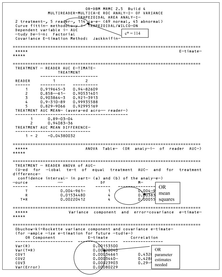
For this study the average spin-echo empirical AUC was .044 larger than the average cine empirical AUC (spin-echo average = 0.941, cine average = 0.897); however, there was not a significant difference (p = 0.0517) between the modalities based on either a DBM or the equivalent OR analysis using jackknife error covariance estimation. Suppose that the researcher would like to know what combinations of reader and case sample sizes for a similar study will have at least 0.80 power to detect an absolute difference of 0.05 between the modality AUCs. We show how to determine the smallest case sample size for each of several reader sample sizes that yields 0.80 power for detecting a .05 difference in spin-echo and cinematic AUC, treating the Van Dyke data as pilot data. We set alpha, the probability of a type I error, equal to .05.

3.2 Parameter estimates from pilot data

Partial output from performing an updated OR analysis comparing empirical AUCs using OR-DBM MRMC 2.5 software (available at http://perception.radiology.uiowa.edu/) with jackknife covariance estimation is presented in Table 1. In Table 1 the Estimates section shows the reader AUC estimates, the ANOVA Tables section presents the ANOVA table corresponding to the OR method, and the Variance component and error-covariance estimates section shows both the OR and corresponding DBM variance components estimates. The inputs needed for the sample size program are circled. Table 1 provides all the necessary information for performing sample size estimation for a future study, with output that is needed for the sample-size program labeled.

Table 1.

Partial OR output for ROC AUC analysis of Van Dyke¹⁴ data using OR-DBM MRMC 2.5 software

3.3 Running the sample-size program

The opening window for the sample-size program is shown in Table 2.

Table 2.

First window in sample-size program.

Table 3 shows the Step 1: Specify study design window. Here we have indicated that we want to do sample-size estimation for a factorial study where each reader reads each case using each test. Note that four other designs could have been selected.

Table 3.

Step 1 in sample-size program

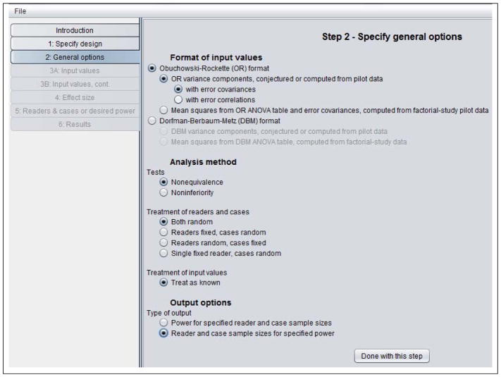
Table 4 shows the Step 2: Specify general options window. Here we have indicated that we will input OR parameter estimates, and we have chosen to input the error covariances rather than the error correlations. Note that we alternatively could have inputted OR means square from the OR analysis. All of the needed inputs are available in Table 1.

Table 4.

Step 2 in sample-size program.

Also, alternatively we could have inputted DBM parameter estimates: either DBM variance components (shown in Table 1) or DBM mean squares. DBM mean squares are not shown in Table 1, but can be obtained by rerunning the OR-DBM MRMC 2.5 analysis and specifying a DBM analysis.

In this window we have requested a nonequivalence test and have requested that both readers and cases be treated as random factors, so that conclusions will generalize to both the reader and case populations. We have also requested various combinations of reader and case sample sizes that will result in .80 power.

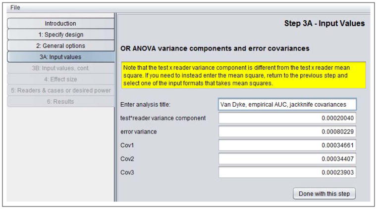
Table 5 shows the Step 3A: Input values window. After entering a descriptive title, we have entered the test-by-reader variance component, the error variance, and Cov1, Cov2, and Cov3 values, all taken from Table 1.

Table 5.

Step 3A in sample-size program.

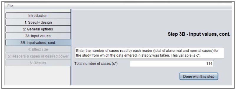
Table 6 shows the Step 3B: Input value, cont window. In this window we have entered c^* = 114, the number of cases in the Van Dyke study, which is also shown in Table 1.

Table 6.

Step 3B in sample-size program.

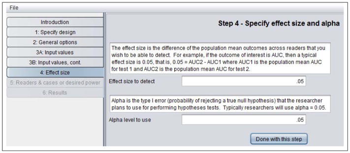
Table 7 shows the Step 4: Specify effect size and alpha window. Here we have indicated the effect size to be an AUC difference of .05 and have set alpha (probability of a type I error) equal to .05 for the sample size computations.

Table 7.

Step 4 in sample-size program.

Table 8 shows the Step 5: Specify readers, cases, and desired power window. Recall that in Step 1 we requested that various combinations of reader and case sample sizes be computed that would result in the specified power. Here we have requested power = .8, and have indicated the program should compute the number of cases needed for between 3 and 10 readers, but with a maximum of 2000 cases; i.e., if the power is not achieved with 2000 cases, then the program does not search for a larger number of cases.

Table 8.

Step 5 in sample-size program.

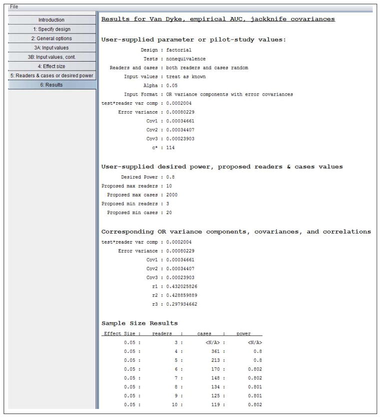
Table 9 shows the Results window. The window first lists the user-supplied values, followed by the Corresponding OR variance components, covariance, and correlations section; we supplied all of the values in this second section except for the correlations (r1, r2, r3). However, if we had inputted mean squares, all of the values in this second section would have been computed by the program.

Table 9.

Results from sample-size program.

The Sample Size Results section shows the number of cases needed to yield 0.80 power as the number of readers varies between 3 and 10. For example, we see that with 6 readers we need 170 cases, and with 5 readers we need 213 cases. We see that for 3 readers the number of cases needed was not less than 2000, as indicated by “<N/A>.”

3.4 Abnormal-to-normal case ratio

Note that the program did not ask for the ratio of abnormal to normal cases, but rather only for the total number of cases for our pilot data. This is because the sample size results assume the same abnormal-to-normal case ratio as for the pilot data, which for the Van Dyke data is 45:69. We would need fewer total cases if we planned to use an equal ratio of abnormal and normal cases for our future study because that is a more efficient design. There are several solutions to this problem. First of all, if the ratio for the planned study will be closer to 1 than it was for the pilot study, then sample size estimates will be conservative and hence can still be used, although they will tend to be larger than needed. However, if the ratios do not differ greatly, then this approach is reasonable. Second, for the situation where the pilot sample ratio is much different from that of the planned study, Hillis et al⁸ have discussed how to revise the pilot-study estimates.

4. Conclusions

The software is a valuable tool for sizing radiologic diagnostic studies because of its ease of use and options for study designs, types of hypotheses, input formats, output formats, and applicability to parametric and nonparametric reader-performance outcomes which can include outcomes from ROC, FROC, and ROI analyses.

References

- 1.Dorfman DD, Berbaum KS, Metz CE. Receiver operating characteristic rating analysis: generalization to the population of readers and patients with the jackknife method. Investigative Radiology. 1992;27(9):723–731. [PubMed] [Google Scholar]
- 2.Dorfman DD, Berbaum KS, Lenth RV, Chen YF, Donaghy BA. Monte Carlo validation of a multireader method for receiver operating characteristic discrete rating data: factorial experimental design. Academic Radiology. 1998;5(9):591–602. doi: 10.1016/s1076-6332(98)80294-8. [DOI] [PubMed] [Google Scholar]
- 3.Obuchowski NA, Rockette HE. Hypothesis testing of diagnostic accuracy for multiple readers and multiple tests: an ANOVA approach with dependent observations. Communications in Statistics-Simulation and Computation. 1995;24(2):285–308. [Google Scholar]
- 4.Hillis SL, Obuchowski NA, Schartz KM, Berbaum KS. A comparison of the Dorfman-Berbaum-Metz and Obuchowski-Rockette Methods for receiver operating characteristic (ROC) data. Statistics in Medicine. 2005;24:1579–1607. doi: 10.1002/sim.2024. [DOI] [PubMed] [Google Scholar]
- 5.Hillis SL. A comparison of denominator degrees of freedom methods for multiple observer ROC analysis. Statistics in Medicine. 2007;26(3):596–619. doi: 10.1002/sim.2532. [DOI] [PMC free article] [PubMed] [Google Scholar]
- 6.Hillis SL, Berbaum KS, Metz CE. Recent developments in the Dorfman-Berbaum-Metz procedure for multireader ROC study analysis. Academic Radiology. 2008;15:647–661. doi: 10.1016/j.acra.2007.12.015. [DOI] [PMC free article] [PubMed] [Google Scholar]
- 7.Hillis SL. A marginal-mean ANOVA approach for analyzing multireader multicase radiological imaging data. Statistics in Medicine. 2014;33(2):330–360. doi: 10.1002/sim.5926. [DOI] [PMC free article] [PubMed] [Google Scholar]
- 8.Hillis SL, Obuchowski NA, Berbaum KS. Power estimation for multireader ROC methods: An updated and unified approach. Academic Radiology. 2011;18(2):129–142. doi: 10.1016/j.acra.2010.09.007. [DOI] [PMC free article] [PubMed] [Google Scholar]
- 9.Bunch PC, Hamilton JF, Sanderson GK, Simmons AH. Free-Response Approach to the Measurement and Characterization of Radiographic-Observer Performance. Journal of Applied Photographic Engineering. 1978;4(4):166–171. [Google Scholar]
- 10.Chakraborty DP, Berbaum KS. Observer studies involving detection and localization: Modeling, analysis, and validation. Medical Physics. 2004;31(8):2313–2330. doi: 10.1118/1.1769352. [DOI] [PubMed] [Google Scholar]
- 11.Obuchowski NA, Lieber ML, Powell KA. Data analysis for detection and localization of multiple abnormalities with application to mammography. Academic Radiology. 2000;7(7):516–525. doi: 10.1016/s1076-6332(00)80324-4. [DOI] [PubMed] [Google Scholar]
- 12.DeLong ER, DeLong DM, Clarke-Pearson DL. Comparing the areas under two or more correlated receiver operating characteristic curves: a nonparametric approach. Biometrics. 1988;44(3):837–845. [PubMed] [Google Scholar]
- 13.Chen W, Petrick NA, Sahiner B. Hypothesis testing in noninferiority and equivalence MRMC ROC studies. Academic Radiology. 2012;19(9):1158–1165. doi: 10.1016/j.acra.2012.04.011. [DOI] [PubMed] [Google Scholar]
- 14.Van Dyke CW, White RD, Obuchowski NA, Geisinger MA, Lorig RJ, Meziane MA. Cine MRI in the diagnosis of thoracic aortic dissection. 79th RSNA Meetings; Chicago, IL. November 28 - December 3 (1993). [Google Scholar]