SLDAssay: A Software Package and Web Tool for Analyzing Limiting Dilution Assays

Abstract

Serial limiting dilution (SLD) assays are used in many areas of infectious disease related research. This paper presents SLDAssay, a free and publicly available R software package and web tool for analyzing data from SLD assays. SLDAssay computes the maximum likelihood estimate (MLE) for the concentration of target cells, with corresponding exact and asymptotic confidence intervals. Exact and asymptotic goodness of fit p-values, and a bias-corrected (BC) MLE are also provided. No other publicly available software currently implements the BC MLE or the exact methods. For validation of SLDAssay, results from Myers et al. (1994) are replicated. Simulations demonstrate the BC MLE is less biased than the MLE. Additionally, simulations demonstrate that exact methods tend to give better confidence interval coverage and goodness-of-fit tests with lower type I error than the asymptotic methods. Additional advantages of using exact methods are also discussed.

1 Introduction

Serial limiting dilution (SLD) assays have been used to estimate the frequency or concentration of a particular cell type in a population for more than a century. In immunology, limiting dilution assays were popularized as a technique to study B-cells and T-cells by Lefkovits and Waldmann (1979) (Hu et al., 2009). Since then, SLD assays have been applied to a variety of immunological studies. For example, SLD assays have been used to estimate the frequency of lymphocyte precursors for a given antigen within blood cells (Macken, 1999), and for comparing depleted and enriched populations in stem cell research (Hu et al., 2009). Other areas where SLD assays have been applied include plant disease assessment (Hepworth, 1996) and estimating the density of coliform bacteria in water samples (Myers et al., 1994).

In current HIV cure research, SLD assays are used to investigate strategies for eradicating the virus from latently infected cells in HIV positive individuals (Archin et al., 2014). In HIV studies, a type of SLD assay known as the quantitative virus outgrowth assay (QVOA) was first used by Finzi et al. (1997) to demonstrate the presence of silent, but replication-competent HIV within a pool of resting CD4+ T cells of durably, anti-retroviral therapy (ART) suppressed individuals. In QVOA, the Poisson distribution is applied to estimate the prevalence of infected resting cells and is reported as infectious units per million (IUPM) resting CD4+ T cells. Several laboratories have used this assay to estimate the frequency of the latent infectious reservoir in different populations of cells, thus confirming that while ART significantly improves the lives of people living with HIV infection, it is ineffective against latent HIV which remains a critical barrier towards HIV eradication (Crooks et al., 2015, Soriano-Sarabia et al., 2015). With the increased effort to define modalities to eliminate persistent HIV infection, SLD assays provide an essential tool to measure the effectiveness of anti-latency interventions. Thus any improvement on methods to better quantitate data from SLD assays such as the QVOA is valuable.

To that end, we present here the development of SLDAssay, a simple, free, publicly available R software package and web tool to analyze data from SLD assays. SLDAssay computes maximum likelihood estimates (MLEs) and bias-corrected (BC) MLEs for the probability a cell is infected or IUPM, with corresponding exact and asymptotic confidence intervals (CI). Exact and asymptotic goodness of fit p-values (PGOF), which may aid in identifying technical problems with the assay, are also provided. No other publicly available software currently implements the BC MLE or the exact methods.

The remainder of this paper is organized as follows. Section 2.1 introduces mathematical notation and terminology, and gives a detailed description of the statistical methods used for calculation of the MLEs, CIs, and PGOFs. Both the exact and asymptotic methods available in SLDAssay are described. Section 2.2 presents a user’s guide for the SLDAssay R package, with example input and output. For validation, Section 2.3 compares the SLDAssay’s results with those from Myers et al. (1994). Section 2.4 gives a brief description of the SLDAssay web tool. Section 3 compares the corrected and uncorrected MLEs, and the exact and asymptotic CIs and PGOFs through simulations. Section 3 also includes simulations that demonstrate the validity of applying Monte Carlo sampling in the exact methods. The SLDAssay R package can be downloaded from CRAN (https://CRAN.R-project.org/package=SLDAssay), and the web tool can be accessed at https://iupm.shinyapps.io/sldassay/.

2 Materials and Methods

2.1 Statistical Considerations

In a SLD assay, the original sample is divided into subsamples at lower concentrations by dilution, creating multiple dilution levels. At each dilution level, the subsample is further divided into a number of identical replicate wells. Each well is tested for the presence of the target organism, which can be recorded as a binary outcome equal to 1 if at least one target organism is present and 0 if no target organisms are present. The result of one SLD assay can be represented as a vector containing the number of positive wells at each dilution level (Figure 1). Intuitively, results from an SLD assay can be used to estimate the concentration of target organisms by using information gained from the proportion of positive wells changing as the number of cells at each dilution level decreases. A large range of dilutions is typically used to increase the likelihood that low dilution wells are positive and high dilution wells are negative. In HIV studies, the number of infectious units per million (IUPM) is often the main parameter of interest.

Figure 1.

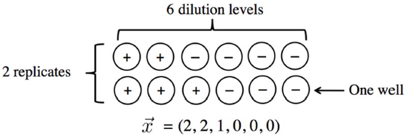
An example SLD assay with 6 dilution levels and 2 replicates per dilution level. The first dilution level could contain one million cells per well, with each progressive level diluting by a factor of 5. Positive wells indicate the presence of at least one infectious unit. Negative wells indicate no infectious units present. The resulting vector, $\overrightarrow{x}$, is the number of positive wells at each dilution level.

In order to estimate the concentration of infected cells, SLDAssay uses a statistical model for a SLD assay with n_d replicates per dilution level and D dilution levels, which employs the Poisson approximation to the binomial (Myers et al., 1994). This model relies on the following four assumptions: the cells in the sample are selected randomly from the larger population of total cells, the infected cell frequency is near zero, the infected cells are distributed randomly amongst wells, and a well will test positive if and only if the well contains at least one infected cell (i.e., the assay has perfect sensitivity and specificity). Supposing these assumptions hold, the probability that a well at the d-th dilution level contains no IUs is (1 − C)^u_d, where C is the probability a cell is infected, and u_d is the number of cells per well at the d-th dilution level. Applying the Poisson approximation, (1 − C)^u_d ≈ exp(−Cu_d). This approximation is accurate for u_d large and C small; a general rule of thumb is u_d ≥ 20 and C ≤ 0.1 (van Belle et al., 2004). Thus, if the approximation holds, the probability that a well contains at least one IU, and is therefore positive, is 1 − exp(−Cu_d). IUPM is then defined as τ = C · 10⁶ While the following methods are described in terms of IUPM, the statistical methods described below may also be used to draw inference about C.

Assuming that all wells are independent, at dilution level d, the number of positive wells x_d out of n_d replicates is binomially distributed with success probability 1 − exp(−Cu_d). Letting $\overrightarrow{x}=(x_1,\dots ,x_d)$ denote the vector of the number of positive wells at each dilution level, the likelihood function is (Fisher, 1922; Myers et al., 1994):

$$L(\tau ;\overrightarrow{x})={\prod _{d=1}^D\left(\begin{array}{c}{n}_d\\ x_d\end{array}\right){\{1-\exp (-\frac{\tau }{{10}^6}{u}_d)\}}^{x_d}\{\exp (-\frac{\tau }{{10}^6}{u}_d)\}}^{n_d-x_d}$$ (1)

In order to obtain the maximum likelihood estimate (MLE) for IUPM, the log of the likelihood function (1) is maximized with respect to τ for a given observed outcome vector $\overrightarrow{x}$; the resulting MLE is denoted τ̂. SLDAssay uses the optim function in R (R Core Team, 2015) to numerically maximize the log likelihood function and obtain τ̂.

The MLE obtained from maximizing (1) is known to be upwardly biased (Hepworth, 1996). To address this, SLDAssay also provides a bias-corrected (BC) MLE described by Hepworth and Watson (2009). The BC MLE utilizes a general bias adjustment described by Gart (1991); thus Hepworth and Watson refer to the BC MLE as the “Gart-V” estimator. The correction entails subtracting from the MLE an estimator of the second-order bias of the MLE. The bias estimator has a complicated form; see equations (6) and (8) of Hepworth and Watson, and the appendix of Hepworth (2005). Simulations in Section 3 below demonstrate the BC MLE has reduced biased compared to the MLE.

SLDAssay returns both exact and asymptotic MLE CIs and model PGOFs. The PGOF is the probability of an experimental result occurring that is as rare or rarer than the one obtained, assuming that the model is correct. Low values of PGOF (e.g., < 0.05) indicate rare or implausible results, perhaps due to false negative or false positive wells. Samples with a very low PGOF might be considered for retesting. To obtain the exact PGOF, the probability of every possible assay outcome given an IUPM equal to τ̂ is calculated using (1). Denote these probabilities by $p({\overrightarrow{x}}_i\mid \widehat{\tau })=L(\widehat{\tau };{\overrightarrow{x}}_i)$ for i = 1, …, N, where ${\overrightarrow{x}}_i$ is the i^th possible SLD assay outcome for the experimental set up and $N=\prod _{d=1}^D(n_d+1)$ is the total number of possible outcomes. The exact PGOF is equal to the sum of all $p({\overrightarrow{x}}_i\mid \widehat{\tau })$ that do not exceed the probability of the observed outcome given τ̂, i.e.,

$$\mathit{PGOF}=\sum _{i=1}^{N}p({\overrightarrow{x}}_i\mid \widehat{\tau })1\{p({\overrightarrow{x}}_i\mid \widehat{\tau })\le p({\overrightarrow{x}}_{\mathit{obs}}\mid \widehat{\tau })\}$$ (2)

Exact CIs for an observed assay outcome, ${\overrightarrow{x}}_{\mathit{obs}}$, can be constructed by inverting the likelihood ratio test (LRT). This approach entails calculating relative likelihood, which is the likelihood normalized relative to its maximum achievable value. The LRT p-value for the null hypothesis H₀ : τ = τ₀ for any IUPM value τ₀ is defined as (Myers et al., 1994):

$$p({\tau }_0)=\sum _{i=1}^{N}p({\overrightarrow{x}}_i\mid {\tau }_0)\cdot 1\{\frac{p({\overrightarrow{x}}_i\mid {\tau }_0)}{p({\overrightarrow{x}}_i\mid {\widehat{\tau }}_i)}\le \frac{p({\overrightarrow{x}}_{\mathit{obs}}\mid {\tau }_0)}{p({\overrightarrow{x}}_{\mathit{obs}}\mid \widehat{\tau })}\}$$ (3)

Here, τ̂_i is the MLE for outcome ${\overrightarrow{x}}_i$. That is, the LRT p-value is the sum of all outcome likelihoods where the relative likelihood of an outcome does not exceed the relative likelihood of the observed outcome. The null hypothesis is rejected at level α if p(τ₀) < α. Thus, the 1 − α exact CI is computed by testing all possible values of τ₀, and retaining in the interval values where p(τ₀) ≥ α. SLDAssay uses the R function uniroot (R Core Team, 2015) to determine the two IUPM values such that p(τ₀) = α.

In order to calculate asymptotic PGOFs and CIs, large sample approximations are used. The IUPM calculator IUPMStats v1.0 (Rosenbloom et al., 2015) uses these asymptotic methods. To obtain the asymptotic PGOF, the test statistic T is used:

$$T=\sum _{d=1}^D{(x_d-e_d)}^2(\frac{1}{e_d}+\frac{1}{n_d-e_d})$$ (4)

Where e_d = n_d{1 − exp(−τ̂/10⁶u_d)} is the expected number of positive outcomes at the d^th level when τ = τ̂. Assuming wells are independent and the number of positive wells is binomially distributed, T follows a chi-square distribution with D − 1 degrees of freedom, from which the asymptotic PGOF is calculated. A computational limitation of this approach is that as τ̂ becomes large, the quantity exp(−τ̂/10⁶u_d) approaches 0, and consequently e_d approaches n_d. This results in software approximating n_d − e_d as 0, such that evaluating (4) results in dividing by zero so that the asymptotic PGOF cannot be computed for large IUPM MLEs.

To calculate asymptotic CIs, the MLE is assumed to be approximately normal. A 95% Wald CI is calculated based on the estimated standard error from the information matrix of the likelihood function (1) evaluated at the IUPM MLE, τ̂. The chi-square approximation for computing the asymptotic PGOF and the normal approximation for computing the asymptotic CI rely on the number of replicates being large. In implementations of the SLD assay where the number of replicates is not large, the asymptotic PGOF may have inflated type I error and the asymptotic CIs may have coverage lower than the nominal level, as demonstrated empirically in Section 3.

Scenarios where all wells are negative or all wells are positive require special attention. When all wells are negative, the MLE τ̂ is 0, and the estimated standard error based on the observed information is not finite. Thus, the asymptotic CI is non-informative because the interval is the entire parameter space. On the other hand, exact CIs provide informative bounds, i.e., the upper bound on the CI will be finite. For this reason, exact CIs are recommended in the case of all negative wells. An alternative method for computing the CI when all wells are negative entails a Bayesian approach (Rosenbloom et al., 2015). This approach assumes a prior distribution for IUPM, and uses the median posterior estimate with a corresponding one-sided 95% upper limit. A limitation of this method is that analysis results will be dependent on the choice of the prior.

When all wells are positive, the MLE is not finite, and consequently asymptotic CIs cannot be computed, whereas exact CIs provide an informative lower bound. Similarly, the asymptotic PGOF cannot be computed, because the chi-square test statistic T is an indeterminate form (i.e. x_d − e_d = 0 and n_d − e_d = 0, resulting in T = 0/0). On the other hand, the exact PGOF can be computed. These scenarios where all wells are positive or all wells are negative illustrate the utility of using exact methods for the analysis of SLD assays.

The MLEs for each possible outcome of an assay, τ̂_i, i = 1, …, N, are needed to calculate exact PGOFs and CIs. For assays with large numbers of replicates, where the number of possible outcomes is large, this can become computationally expensive. To address this computational issue, SLDAssay provides the user the option of using Monte Carlo sampling to approximate exact PGOFs and CIs. This numerical approximation entails calculating the MLEs only for a subset of randomly selected possible outcomes, and then up-weighting their contribution to (2) and (3) accordingly. Accuracy of results using Monte Carlo sampling is demonstrated with simulations in Section 3.2.

2.2 R package User’s Guide

For R versions 3.2.1 or higher, the SLDAssay package can be installed from CRAN using the command install.packages(“SLDAssay”). The package contains a single function get.mle that takes as arguments:

• pos: Vector of number of positive wells at each dilution level, i.e., $\overrightarrow{x}=(x_1,x_2,\dots ,x_D)$.

• replicates: Vector of number of replicates at each dilution level, i.e., (n₁, n₂, …, n_D).

• dilutions: Vector of number of cells per well at each dilution level, i.e., (u₁, u₂, …, u_D)

• monte: Number of Monte Carlo samples. Default is exact (no sampling), unless more than 15,000 possible well outcomes exist, in which case 15,000 Monte Carlo samples are taken. Use monte=F for exact computation.

• conf.level: Confidence level of the interval.

• iupm: Boolean variable, indicates whether to return MLE of the IUPM (iupm=TRUE) or the probability a cell is infected (iupm=FALSE)

The function get.mle computes the MLE and BC MLE for the IUPM or the probability a cell is infected (MLE and BC MLE), the exact and asymptotic PGOFs (Exact PGOF and Asymp PGOF), and the 100 × (1 − α)% exact and asymptotic CIs (Exact CI and Asymp CI) using the methods described in Section 2.1.

2.3 R package Examples

The following code exemplifies the use of the SLDAssay R package’s main function, get.mle. This code reproduces rows 1-3 and row 15 of Table 4 from Myers et al. (1994). Results comparing SLDAssay and Myers et al. are shown in Table 1.

row1	<-	get.mle(pos=c(0,0,0,0,0,0), replicates=rep(2,6),
		dilutions=c(1e6,2e5,4e4,8e3,1600,320), conf.level=0.95, iupm=T)
row2	<-	get.mle(pos=c(1,0,0,0,0,0), replicates=rep(2,6),
		dilutions=c(1e6,2e5,4e4,8e3,1600,320), conf.level=0.95, iupm=T)
row3	<-	get.mle(pos=c(2,0,0,0,0,0), replicates=rep(2,6),
		dilutions=c(1e6,2e5,4e4,8e3,1600,320), conf.level=0.95, iupm=T)
row15	<-	get.mle(pos=c(2,2,1,1,0,0), replicates=rep(2,6),
		dilutions=c(1e6,2e5,4e4,8e3,1600,320), conf.level=0.95, iupm=T)

Table 4.

Simulation results for assays with 80% sensitivity and specificity.

IUPM	Dilution Levels	Replicates	Mean Bias (SE)		CI Coverage		PGOF Power
			MLE	BC MLE	Exact	Asymptotic	Exact	Asymptotic
8	4	2	1.3 (0.4)	-2.4 (0.2)	0.62	0.63	0.29	0.47
8	4	3	-0.3 (0.3)	-2.4 (0.2)	0.55	0.57	0.45	0.50
8	4	4	-1.6 (0.2)	-2.8 (0.2)	0.49	0.53	0.57	0.62
8	6	2	5.1 (0.8)	0.4 (0.5)	0.57	0.62	0.66	0.72
8	6	3	2.3 (0.5)	-0.2 (0.4)	0.59	0.58	0.82	0.86
8	6	4	0.1 (0.3)	-1.4 (0.3)	0.53	0.58	0.89	0.92

Table 1.

Replication of Table 4 in Myers et al. (1994)

Outcome	MLE		PGOF		CI
	SLDAssay	Myers	SLDAssay	Myers	SLDAssay	Myers
000000	0.000	0.000	1.00000	1.00000	(0.000,1.228)	(0.000, 1.220)
100000	0.511	0.508	1.00000	1.00000	(0.026, 2.742)	(0.026, 2.732)
200000	1.610	1.612	1.00000	1.00000	(0.248, 7.037)	(0.248, 7.031)
210000	3.246	3.235	1.00000	1.00000	(0.633, 13.961)	(0.639, 13.831)
220000	8.079	8.081	1.00000	1.00000	(1.133, 35.333)	(1.138, 35.241)
221000	16.248	16.218	1.00000	1.00000	(2.742, 70.343)	(2.759, 70.021)
222000	40.519	40.509	1.00000	1.00000	(7.036, 180.565)	(7.101, 180.201)
222100	81.699	82.105	1.00000	1.00000	(13.961, 366.769)	(13.969, 365.237)
222200	205.838	205.086	1.00000	1.00000	(35.333, 1,067.474)	(35.594, 1,059.16)
222210	420.553	419.830	1.00000	1.00000	(70.343, 1,653.060)	(70.721, 1,640.98)
222220	1,121.505	1,124.32	1.00000	1.00000	(180.565, 4,712.721)	(182.003, 4,711.59)
222221	2,503.27	2,492.30	1.00000	1.00000	(366.769, 11,487.934)	(368.889, 11,422.7)
222222	∞	∞	1.00000	1.00000	(1,014.015, ∞)	(1,017.83, ∞)
211000	5.656	5.648	0.36269	0.36280	(1.031, 17.779)	(1.041, 17.737)
221100	28.328	28.313	0.36022	0.36027	(6.468, 89.611)	(6.493, 88.908)
110000	1.108	1.105	0.36002	0.36020	(0.188, 3.546)	(0.190, 3.538)
222110	142.867	143.339	0.34765	0.34732	(32.442, 468.180)	(32.545, 463.754)
222211	747.044	747.676	0.27766	0.27752	(164.176, 2,128.673)	(164.765, 2,125.48)
201000	2.827	2.815	0.25410	0.25477	(0.593, 9.017)	(0.596, 9.016)
220100	14.149	14.109	0.25261	0.25305	(2.654, 45.282)	(2.678, 45.195)
222010	71.059	70.721	0.24511	0.24587	(13.514, 231.700)	(13.558, 231.095)
222201	363.367	361.621	0.20563	0.20653	(68.030, 1,381.362)	(68.641, 1,371.88)

Myers et al. use a grid search to compute the MLE. The grid search treats the IUPM parameter space as finite, consisting of 2,779 values from 1.01^−1,389 to 1.01^1,389 (i.e., approximately 10⁻⁷ to 10⁶). In contrast, SLDAssay uses the Brent method in the numerical optimizer optim to search the IUPM parameter space from 10⁻¹⁸ to 10¹⁴ (R Core Team, 2015). Thus, the results from SLDAssay are slightly different than those of Myers et al. These differences are compared in Figure 3. The left panel of Figure 3 plots the SLDAssay MLEs versus the MLEs computed by Myers et al. (1994). All points lie close to the identity line, demonstrating the two MLEs are very similar. The right panel of Figure 3 plots the difference in log likelihoods evaluated at the SLDAssay MLEs minus the Myers et al. (1994) MLEs. All differences are positive, indicating the log likelihood is higher for MLEs computed by SLDAssay. Thus, in each instance the SLDAssay MLE is closer to the true MLE.

Figure 3.

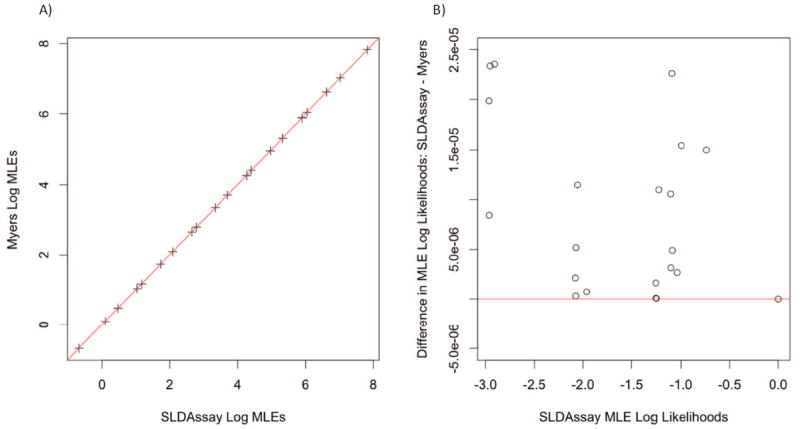
A) Log of SLDAssay MLEs versus log of MLEs computed by Myers et al. (1994). B) Differences in log likelihoods evaluated at SLDAssay MLEs minus Myers et al. (1994) MLEs.

2.4 Web Tool

SLDAssay is also implemented as a user-friendly web tool through the Shiny R package at https://iupm.shinyapps.io/sldassay/ (R Core Team, 2015). To use the web tool, there is no need to download software or perform any programming. The user may input a data table of three columns, corresponding to the number of cells per well, number of replicates, and number of positive wells. Rows may be added or deleted according to the number of dilution levels. The user may also input the number of Monte Carlo samples, the confidence level for the CI, and whether to return the MLEs as IUPM or probability a cell is infected. The output of the web tool is the same as the R package: the MLE, the BC MLE, the exact and asymptotic PGOFs, and the 100 × (1 − α)% exact and asymptotic CIs. Figure 2 illustrates how to use the web tool for the example assay shown in Figure 1.

Figure 2.

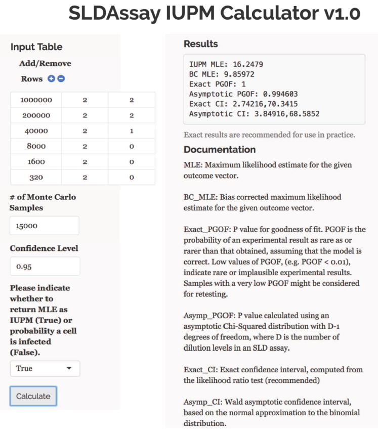
An example of how to use the web tool to analyze the assay described in Figure 1.

3 Results

Simulations were run to compare the BC MLE and MLE, and the exact and asymptotic PGOF and CI described in Section 2.1. Data sets of 10,000 SLD assay outcomes with perfect sensitivity and specificity were generated using the model specified in Section 2.1, a maximum well size of one million cells, a dilution factor of 5, an IUPM value of 8 or 12, 4 or 6 dilution levels, and 2, 3, or 4 replicates per dilution level. For each simulated SLD assay outcome, the IUPM MLE, BC MLE, exact and asymptotic PGOFs, and exact and asymptotic CIs were calculated. Three measures were used to evaluate the performance of the statistical methods:

• Empirical bias: the difference between the arithmetic mean of the MLEs and the true IUPM.

• Empirical standard error (SE): the standard deviation of the empirical bias divided by the square root of the number of simulations. A measure of the accuracy of the bias estimate.

• Empirical type I error or power: the proportion of times the PGOF was less than or equal to the level of significance (i.e., 0.05). For assays simulated to have perfect sensitivity and specificity, this proportion approximates the type I error. For assays simulated with error (described below), this proportion approximates the power.

• Empirical coverage: the percentage of CIs which include the true IUPM.

Table 2 contains results of the simulations. Biases in the range of 1.5 to 5.9 were observed for the MLE, whereas the BC MLE had biases in the range of -1.5 to 0.0. In all scenarios, the exact CIs had coverage that was either equal to or above the nominal level; these results are to be expected given the exact nature of these confidence intervals; i.e., they are guaranteed to have coverage equal to or above the specified level. The asymptotic CIs performed similarly, although coverage was slightly below the nominal level in some scenarios. The exact PGOF did not have any inflated type I error, which is also guaranteed by the exact construction of the test. On the other hand, as a result of relying on asymptotic approximations, the asymptotic PGOF had several instances of inflated type I error.

Table 2.

Simulation results for assays with perfect sensitivity and specificity.

IUPM	Dilution Levels	Replicates	Mean Bias (SE)		CI Coverage		PGOF Type I Error
			MLE	BC MLE	Exact	Asymptotic	Exact	Asymptotic
8	4	2	3.7 (0.1)	-0.8 (0.1)	0.98	0.93	0.01	0.10
8	4	3	2.4 (0.1)	-0.3 (0.1)	0.97	0.97	0.02	0.04
8	4	4	1.6 (0.1)	-0.2 (0.0)	0.95	0.94	0.03	0.03
8	6	2	3.6 (0.1)	-0.5 (0.1)	0.97	0.93	0.03	0.09
8	6	3	2.1 (0.1)	-0.3 (0.1)	0.96	0.96	0.03	0.06
8	6	4	1.5 (0.1)	-0.2 (0.0)	0.96	0.96	0.03	0.06
12	4	2	5.9 (0.2)	-1.5 (0.1)	0.97	0.97	0.01	0.16
12	4	3	4.0 (0.1)	-0.3 (0.1)	0.97	0.94	0.02	0.07
12	4	4	2.8 (0.1)	-0.1 (0.1)	0.96	0.93	0.03	0.05
12	6	2	5.5 (0.2)	-0.7 (0.1)	0.97	0.96	0.03	0.16
12	6	3	3.4 (0.1)	-0.3 (0.1)	0.97	0.97	0.03	0.10
12	6	4	2.6 (0.1)	0.0 (0.1)	0.96	0.93	0.03	0.08

Additionally, data sets of 1,000 outcomes with perfect sensitivity and specificity were generated using a true IUPM of 0.5, 2 or 3 replicates, and 4 or 6 dilution levels. Results are shown in Table 3. With a true IUPM equal to 0.5, the simulations produce many outcomes with all negative wells. In the case of all negative wells, the asymptotic CIs are non-informative, i.e. equal to (0, ∞). While both exact and asymptotic methods demonstrate similar empirical coverage, the asymptotic intervals provide coverage that is non-informative for a significant portion of results, whereas by construction the exact CIs always provide informative bounds. The BC MLEs once again have less bias than the MLEs.

Table 3.

Simulation results for assays generated with perfect sensitivity and specificity and IUPM equal to 0.5. The proportion of non-informative CIs, i.e., (0, ∞), is shown. Exact CIs were never non-informative.

Dilution Levels	Replicates	Mean Bias (SE)		CI Coverage		PGOF Type I Error
		MLE	BC MLE	Exact	Asymptotic (% non-informative)	Exact	Asymptotic
4	2	0.2 (0.0)	0.0 (0.0)	0.95	0.95 (0.30)	0.02	0.04
4	3	0.1 (0.0)	0.0 (0.0)	0.97	0.97 (0.17)	0.01	0.05
6	2	0.2 (0.0)	0.0 (0.0)	0.96	0.96 (0.29)	0.03	0.04
6	3	0.1 (0.0)	0.0 (0.0)	0.97	0.97 (0.15)	0.02	0.06

In addition to simulations with perfect sensitivity and specificity, two simulations of 1,000 outcomes were generated with error introduced into the assay outcomes. First, assay results with 80% sensitivity and specificity, i.e., where wells had a 0.8 probability of being correctly identified as positive or negative, were produced with a true IUPM of 8 and varying dilution levels and replicates. Second, assay results were produced with varying sensitivity and specificity, an IUPM equal to 8, 4 dilution levels, and 3 replicates per dilution level. Results are shown in Tables 4 and 5, respectively. For these simulations, the proportion of times the PGOF is less than or equal to 0.05 approximates the statistical power of the PGOF test, i.e., the probability of rejecting the null hypothesis of no error when the null hypothesis is false. Although the asymptotic methods have higher power to detect a true lack of fit, they do not control type I error, as shown in Table 2. Results in Tables 4 and 5 also demonstrate (i) power to detect lack of fit increases with increasing number of replicates and dilution levels, and (ii) both the MLE and BC MLE can have appreciable bias when sensitivity or specificity is low (<90%).

Table 5.

Simulation results under varying sensitivities and specificities for assays with IUPM equal to 8, 4 dilutions levels, and 3 replicates per dilution level.

Specificity	Sensitivity	Mean Bias (SE)		CI Coverage		PGOF Power
		MLE	BC MLE	Exact	Asymptotic	Exact	Asymptotic
80	80	-0.3 (0.3)	-2.4 (0.2)	0.55	0.57	0.45	0.50
80	90	3.2 (0.4)	0.2 (0.3)	0.73	0.74	0.31	0.37
80	100	8.9 (0.5)	4.3 (0.3)	0.83	0.83	0.12	0.19
90	80	-2.4 (0.3)	-3.8 (0.2)	0.50	0.51	0.32	0.38
90	90	0.8 (0.3)	-1.4 (0.2)	0.74	0.75	0.22	0.27
90	100	5.4 (0.4)	1.9 (0.2)	0.91	0.91	0.07	0.11
100	75	-4.1 (0.1)	-5.0 (0.1)	0.41	0.41	0.23	0.26
100	80	-3.3 (0.1)	-4.4 (0.1)	0.52	0.52	0.19	0.22
100	85	-2.4 (0.2)	-3.8 (0.1)	0.64	0.64	0.17	0.20
100	90	-0.9 (0.2)	-2.7 (0.1)	0.74	0.74	0.12	0.15
100	95	0.7 (0.2)	-1.5 (0.2)	0.86	0.86	0.07	0.10
100	100	2.2 (0.2)	-0.4 (0.2)	0.98	0.98	0.02	0.04

To investigate the operating characteristics of the Monte Carlo sampling option in SLDAssay, an assay with 4 dilution levels, (36, 36, 6, 6) replicates per dilution level, (2,500,000, 500,000, 100,000, 25,000) cells per well per dilution level, and an IUPM of 0.5 was simulated 1,000 times with perfect sensitivity and specificity. SLDAssay was used to analyze this data set with and without varying Monte Carlo sampling fractions. Results are shown in Table 6. The total number of possible outcomes, N, is equal to 67,081. With the use of 15,000 Monte Carlo samples, which is a sampling fraction of 0.224, the computation time is reduced, with only a small penalty in coverage and no change in type I error. When Monte Carlo sampling is necessary, SLDAssay users are recommended to set the number of Monte Carlo samples as large as computationally feasible.

Table 6.

Simulation results for IUPM equal to 0.5, 4 dilution levels, (36, 36, 6, 6) replicates per dilution level, (2,500,000, 500,000, 100,000, 25,000) cells per well per dilution level, and various Monte Carlo sampling fractions.

Monte Carlo Samples	Sampling Fraction	Type I Error	Coverage
None	1.00	0.03	0.95
15,000	0.22	0.03	0.94
10,000	0.15	0.03	0.95
5,000	0.08	0.03	0.95
2,500	0.04	0.02	0.92
1,000	0.02	0.03	0.90

4 Discussion

SLDAssay is a free, publicly available, user-friendly R package and web tool available to researchers conducting SLD assays. This software can be used to calculate the MLE and BC MLE for IUPM or probability a cell is infected from a SLD assay, along with both asymptotic and exact CIs and PGOFs. Simulations demonstrate the BC MLE is less biased than the MLE. Simulations also show the exact methods provide better coverage and lower type I error when compared to the asymptotic methods, and so these exact methods are recommended.

References

- 1.Archin NM, Bateson R, Tripathy MK, Crooks AM, Yang KH, Dahl NP, Kearney MF, Anderson EM, Coffin JM, Strain MC, et al. HIV-1 expression within resting CD4+ T-cells after multiple doses of vorinostat. Journal of Infectious Diseases. 2014;210(5):728–735. doi: 10.1038/nrmicro3352. [DOI] [PMC free article] [PubMed] [Google Scholar]
- 2.van Belle G, Fisher LD, Heagerty PJ, Lumley T. Biostatistics: A Methodology for the Health Sciences. 2. Wiley; 2004. [Google Scholar]
- 3.Crooks AM, Bateson R, Cope AB, Dahl NP, Griggs MK, Kuruc JD, Gay CL, Eron JJ, Margolis DM, Bosch RJ, Archin NM. Precise Quantitation of the Latent HIV-1 Reservoir: Implications for Eradication Strategies. Journal of Infectious Disease. 2015 Nov 1;212(9):1361–5. doi: 10.1093/infdis/jiv218. [DOI] [PMC free article] [PubMed] [Google Scholar]
- 4.Finzi D, Hermankova M, Pierson T, Carruth LM, Buck C, Chaisson RE, Quinn TC, Chadwick K, Margolick J, Brookmeyer R, Gallant J, Markowitz M, Ho DD, Richman DD, Silicano RF. Identification of a reservoir for HIV-1 in patients on highly active antiretroviral therapy. Science. 1997;278(5341):1295–300. doi: 10.1126/science.278.5341.1295. [DOI] [PubMed] [Google Scholar]
- 5.Fisher RA. On the Mathematical Foundations of Theoretical Statistics. Phil Trans R Soc A. 1922;222:309–68. [Google Scholar]
- 6.Gart JJ. An application of score methodology: confidence intervals and tests of fit for one-hit curves. Handbook of Statistics. 1991;8:395–406. [Google Scholar]
- 7.Hepworth G. Exact confidence intervals for proportions estimated by group testing. Bio-metrics. 1996;52(3):1134–1146. doi: 10.2307/2533075. [DOI] [Google Scholar]
- 8.Hepworth G. Confidence Intervals for Proportions Estimated by Group Testing With Groups of Unequal Size. Journal of Agricultural, Biological, and Environmental Statistics. 2005;10(4):478–497. [Google Scholar]
- 9.Hepworth G, Watson R. Debiased estimation of proportions in group testing. Applied Statistics. 2009;58(1):105–121. [Google Scholar]
- 10.Hu L, Smyth GK. ELDA: Extreme limiting dilution analysis for comparing depleted and enriched populations in stem cell and other assays. Journal of Immunological Methods. 2009;347(1-2):70–78. doi: 10.1016/j.jim.2009.06.008. [DOI] [PubMed] [Google Scholar]
- 11.Lefkovits I, Waldmann H. Limiting Dilution Analysis of the Immune System. Cambridge University Press; Cambridge: 1979. [Google Scholar]
- 12.Macken C. Design and analysis of serial limiting dilution assays with small sample sizes. Journal of Immunological Methods. 1999;222(1-2):13–29. doi: 10.1016/S0022-1759(98)00133-1. [DOI] [PubMed] [Google Scholar]
- 13.Myers LE, McQuay LJ, Hollinger FB. Dilution assay statistics. Journal of Clinical Microbiology. 1994;32(3):732–739. doi: 10.1128/jcm.32.3.732-739.1994. [DOI] [PMC free article] [PubMed] [Google Scholar]
- 14.R Core Team. R: A Language and Environment for Statistical Computing. R Foundation for Statistical Computing; Vienna, Austria: 2015. URL: http://www.R-project.org/ [Google Scholar]
- 15.Rosenbloom DS, Elliot O, Hill AL, Henrich TJ, Siliciano JM, Siliciano RF. Designing and interpreting limiting dilution assays: general principles and applications to the latent reservoir for human immunodeficiency virus-1. Open Forum Infectious Diseases. 2015;2(4) doi: 10.1093/ofid/ofv123. ofv123. [DOI] [PMC free article] [PubMed] [Google Scholar]
- 16.Soriano-Sarabia N, Archin NM, Bateson R, Dahl NP, Crooks AM, Kuruc JD, Garrido C, Margolis DM. Peripheral Vγ9Vδ2 T Cells Are a Novel Reservoir of Latent HIV Infection. PLoS Pathog. 2015 Oct 16;11(10):e1005201. doi: 10.1371/journal.ppat.1005201. [DOI] [PMC free article] [PubMed] [Google Scholar]