

Abstract
Purpose
Colitis refers to inflammation of the inner lining of the colon that is frequently associated with infection and allergic reactions. In this paper, we propose deep convolutional neural networks methods for lesion‐level colitis detection and a support vector machine (SVM) classifier for patient‐level colitis diagnosis on routine abdominal CT scans.
Methods
The recently developed Faster Region‐based Convolutional Neural Network (Faster RCNN) is utilized for lesion‐level colitis detection. For each 2D slice, rectangular region proposals are generated by region proposal networks (RPN). Then, each region proposal is jointly classified and refined by a softmax classifier and bounding‐box regressor. Two convolutional neural networks, eight layers of ZF net and 16 layers of VGG net are compared for colitis detection. Finally, for each patient, the detections on all 2D slices are collected and a SVM classifier is applied to develop a patient‐level diagnosis. We trained and evaluated our method with 80 colitis patients and 80 normal cases using 4 × 4‐fold cross validation.
Results
For lesion‐level colitis detection, with ZF net, the mean of average precisions (mAP) were 48.7% and 50.9% for RCNN and Faster RCNN, respectively. The detection system achieved sensitivities of 51.4% and 54.0% at two false positives per patient for RCNN and Faster RCNN, respectively. With VGG net, Faster RCNN increased the mAP to 56.9% and increased the sensitivity to 58.4% at two false positive per patient.
For patient‐level colitis diagnosis, with ZF net, the average areas under the ROC curve (AUC) were 0.978 ± 0.009 and 0.984 ± 0.008 for RCNN and Faster RCNN method, respectively. The difference was not statistically significant with P = 0.18. At the optimal operating point, the RCNN method correctly identified 90.4% (72.3/80) of the colitis patients and 94.0% (75.2/80) of normal cases. The sensitivity improved to 91.6% (73.3/80) and the specificity improved to 95.0% (76.0/80) for the Faster RCNN method. With VGG net, Faster RCNN increased the AUC to 0.986 ± 0.007 and increased the diagnosis sensitivity to 93.7% (75.0/80) and specificity was unchanged at 95.0% (76.0/80).
Conclusion
Colitis detection and diagnosis by deep convolutional neural networks is accurate and promising for future clinical application.
Keywords: colitis detection, colitis diagnosis, Region‐based CNN, RPN
1. Introduction
Colitis is inflammation of the inner lining of the colon wall that can often lead to diarrhea and abdominal pain. This inflammation can be caused by ischemia, infection, neutropenia, or irritable bowel disease (ulcerative colitis and Crohn disease).1 Abdominal computer tomography (CT) is commonly used to diagnose colitis in patients that present with these symptoms.
The wall thickness of a healthy colon is less than 3 mm and often imperceptible if the colon is fully distended.2 Any measure higher than that is often considered a clinical abnormality.1 Aside from indicating the presence of colitis, colon wall thickness has been proven to hold clinical significance in diagnoses of tumors or inflammatory conditions.3 In a study of using CT scans for differential diagnoses, the average colon wall thickness was 11.0 mm in patients with Crohn Disease. For patients with ulcerative colitis, the average colon wall thickness was 7.8 mm.4
Another indicator of colitis in CT scans is the “accordion” sign. The accordion sign is seen on CT images of patients with oral contrast material and refers to the similarity between the thickened walls of colitis to that of an accordion. Its appearance arises as a result of the oral contrast being trapped between thickened edematous haustral folds and mucosal ridges.4, 5, 6 Figure 1 shows examples of normal colon, thickened colon wall and the accordion sign on CT scans. The thickened colon wall and accordion pattern are important for computer‐aided detection of colitis.
Figure 1.

(a) Normal colon with wall thickness less than 3 mm (green arrow). (b) Colitis of the cecum with wall thickening measured as 10.6 mm (red arrows). (c) Colitis of the ascending with accordion sign (red arrows). [Color figure can be viewed at wileyonlinelibrary.com]
In treating colitis, early detection is critical to early intervention that lessens the negative impact of the ailment. Currently, CT images are manually examined to detect colitis, which is tedious and inefficient. Therefore, computer‐aided colitis detection could greatly reduce the radiologists’ workload and could be employed as a first or second reader for improved disease assessment.
Recent breakthroughs in object detection in computer vision are driven by the success of deep convolutional neural networks (CNNs).7 CNNs can effectively recognize and classify images using hierarchical image representations (CNN features). These hierarchical features have been found to be more efficient for object detection and recognition than handcrafted features such as HOG8 and SIFT.9 The fact that CNNs do not require handcrafted features is a very desirable property of these neural networks and makes them useful for medical image analysis applications.
CNNs and other deep learning methods have been applied to a wide variety of applications in medical imaging.10 Roth et al.11 apply CNNs to improve lymph nodes detection on body CT scans. They decompose the original 3D image to 2D patches in three orthogonal directions, and up to 100 randomly rotated views (“2.5D” views). The CNN predictions on these 2.5D views are later aggregated to attain significant gains in accuracy. Dou et al.12 detect cerebral micro‐bleeds from MRI scans using a two‐stage 3D CNNs. Method with their 3D CNN outperforms the various classical and 2D CNN approaches. Ghesu et al.13 combine deep learning and marginal space learning for object detection and segmentation on cardiac ultrasound scans. They enforce sparsity into the deep networks to increase computational efficiency and reduce segmentation error. Brosch et al.14 develop a 3D deep convolutional encoder network for multiple sclerosis brain lesion segmentation on MRI scans. They combine interconnected convolutional pathway for learning high level features and deconvolutional pathway for predicting the voxel level segmentation. Their results are comparable to the best state‐of‐the‐art methods.
In our previous work,15, 16 we investigated automated methods for colitis detection in CT images. A visual codebook with hand‐crafted features (Gabor filters) and support vector machines were proposed to detect and classify colitis regions.15 This non‐CNN based method required the segmentation of muscle, kidneys, and liver to reduce the false detections. However, the segmentation of these organs itself is challenging in CT images. In,16 we proposed colitis detection using a region‐based convolutional neural network (RCNN) method, which provided better performance and did not require prior organ segmentations.
Object detection by the RCNN is slow because it performs a forward pass for each region proposal and does not share the computation among the region proposals. One of the latest RCNN advances, Faster RCNN,7 can achieve nearly real‐time rates using very deep networks. In this work, we extend our previous colitis RCNN detection method16 by applying a Faster RCNN architecture for colitis detection and achieve improved both accuracy and efficiency. In addition, a separate support vector machine classifier is then utilized at the patient level to diagnose if the patient has colitis.
2. Methods
2.A. Colitis detection by RCNN
For completeness, our prior work on colitis detection using RCNN is summarized here in Fig. 2. The colitis detection by RCNN has four steps. First, for each input image, category‐independent region proposals (rectangular boxes) are generated with selective search.17 These region proposals are potential candidates for colitis detection. Second, each region proposal is warped by linear interpolation to the required size of a CNN architecture and a fixed‐length (4096 dimensional) feature vector is computed using a CNN architecture. Third, a support vector machine (SVM) is utilized for colitis classification. Finally, potential colitis detections are refined using bounding‐box regression.
Figure 2.

Colitis Detection by RCNN. Input image: a transverse CT slice through the abdomen of a patient with colitis. This patient has received both oral and intravenous contrast material. (1). Region proposals (orange boxes) are generated by selective search. (2). CNN features are computed using a deep CNN. (3). After CNN feature computation, an SVM classifies each region as colitis or not. (4). After the SVM classification, each region proposal is refined (green box) by bounding‐box regression. [Color figure can be viewed at wileyonlinelibrary.com]
A class‐specific linear regression model is trained for bounding‐box regression. A region proposal R is defined with four coordinates as:
| (1) |
where R x , R y , R w , and R h denote the coordinates of center, width, and height of R. Each ground‐truth bounding‐box G is defined in the same way:
| (2) |
A transformation is learned to map a region proposal R to a ground‐truth bounding‐box G.
This transformation is parameterized with four functions , , , and . After learning these functions, a refined bounding‐box is defined as:
| (3) |
| (4) |
| (5) |
| (6) |
Each function of , , , and is modeled as a linear function of the CNN features of region proposal R. More details about learning these functions by optimizing the regularized least squares objective can be found in Ref. 18.
In the colitis detection by RCNN, training is required in three individual stages. First, the CNN is trained and fine‐tuned on region proposals using a log loss function. Second, the SVM is trained for colitis classification on each region proposal using the CNN features as input. Third, a bounding‐box regressor is trained to refine the locations of detected colitis. Figure 2 shows that colitis detection by RCNN is computationally expensive because it performs a forward pass for each individual region proposal in the second step. Thus the feature extraction of all region proposals within the input image does not share the forward pass computations.
2.B. Colitis detection by Faster RCNN
In this work, we use the recent advanced Faster RCNN for colitis detection. The Faster RCNN has three major advantages compared to the previous colitis detection by RCNN: (a) Instead of the inefficient multiple training process within the RCNN, the Faster RCNN employs an efficient single‐stage training process and jointly learns to classify colitis proposals and refine their spatial locations. (b) Compared to around 3000 region proposals per image generated by selective search in RCNN, only around 300 high quality region proposals per image are generated by the region proposal network (RPN) in Faster RCNN. (c) Unlike CNN feature extraction, which is performed on each region proposal individually in RCNN, in Faster RCNN, a forward pass is performed on the entire input image to create one feature map. The features of region proposals are computed by the region‐of‐interest (ROI) projection in the feature map. The computational cost on each ROI is negligible.
Figure 3 shows the overview of colitis detection by Faster RCNN. Input images are all transverse CT slices through the abdomen of a patient. For each slice, region proposals are generated by RPN. Each region proposal is then jointly classified and refined by softmax classification and bounding‐box regression. For each patient, the detections on all slices are collected for patient‐level diagnosis using an SVM classifier. More details about patient‐level classification for diagnosis are discussed in Section 2.C.
Figure 3.

Colitis detection by Faster RCNN. Input images are all transverse CT slices through the abdomen of a patient. (1). For each slice, region proposals (orange boxes) are generated by RPN. (2). Each region proposal is jointly classified and refined (green box) by softmax classification and bounding‐box regression. (3). For each patient, the detections on all slices are collected for patient‐level diagnosis using an SVM classifier.
2.B.1. Region proposal network
Many recent studies19, 20 proposed methods for generating category‐independent region proposals. In our previous work,16 we used a selective search approach17 to generate region proposals because of its computational accuracy and efficiency. An efficient graph‐based algorithm was first used to obtain initial regions. Then, a grouping method17 was used to iteratively group regions as proposals. In our experiment, we used around 3000 region proposals for each image output by selective search.
In this work, Region Proposal Networks (RPN), a fully convolutional architecture, are used to create region proposals. For an input image (of any size), RPN outputs a set of rectangular region proposals and their objectness score. Objectness is the probability of the region proposal to be one of the object classes.
In RPN, to generate region proposals, a small (3 × 3) window slides over the feature map from the last shared convolutional layer (shared between the RPN and the detection network). Each window of the convolutional feature map is mapped to a fixed‐length feature vector. This feature is fed into two fully connected layers, a bounding‐box regression layer and a classification layer. As suggested in,7 at each sliding‐window location, nine region proposals (three aspect ratios and three scales) are predicted. So, the regression layer has 4 × 9 outputs (coordinates of two corners of nine boxes) and the classification layer outputs 2 × 9 scores (the probability of object or background). An objective function7 with multitask loss was minimized.
The RPN was trained end‐to‐end using backpropagation and optimized with stochastic gradient descent (SGD). In each SGD iteration, a mini‐batch (128 positive samples and 128 negative samples from the same image) was constructed for loss optimization. All ground‐truth bounding boxes of the colitis and the region proposals with IoU (intersection over union) ≥ 0.6 are defined as positive samples. Negative samples are defined as the region proposals with IoU ≤ 0.1. The region proposals with IoU between 0.1 and 0.6 are ignored to reduce the classification uncertainty. Caffe21 implementation of an eight‐layer ZF net22 was used for most results in this work. The RPN are initialized by an ImageNet pretrained model.20 All layers of the ZF net are fine‐tuned with a learning rate of 0.0001, a weight decay of 0.0005, and a momentum of 0.9 for 20 k mini‐batches on our colitis dataset.
Compared to around 3000 region proposals per image by the selective search in RCNN, 300 high quality region proposals per image are generated by the RPN in Faster RCNN. Figure 4 shows some examples of the generated region proposals with objectness score.
Figure 4.
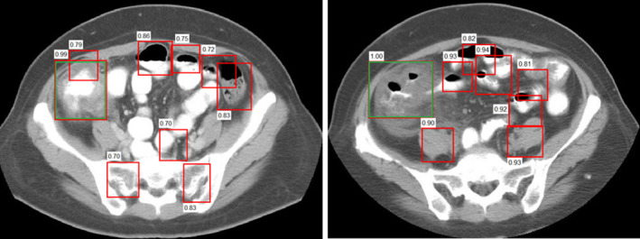
Two examples of generated region proposals (red boxes) with their objectness score by RPN and manually labeled colitis (green boxes) for two different patients. [Color figure can be viewed at wileyonlinelibrary.com]
2.B.2. Detection networks
We use Fast RCNN23 as the detection network in our algorithm. A four‐step training method7 is utilized to learn the shared convolutional layers between the RPN and detection network. First, the RPN is initialized with a pretrained model (using ImageNet). All layers are fine‐tuned for region proposal generation. Second, a separate detection network is also initialized with a pretrained model (using ImageNet) and is trained using the proposals generated in the first step. Third, the RPN was initialized by the detection network. The shared convolutional layers are fixed and the layers of RPN are fine‐tuned. Finally, keeping the shared convolutional layers, the fully connected layers of the detection network are fine‐tuned. In this way, RPN and detection networks form a unified network by sharing the same convolutional layers.
2.C. Patient‐level diagnosis
CT is the primary screening modality for patients suspected of having colitis. The enhancement pattern, degree of mural thickening, and the length of colon involvement are important imaging features for diagnosis of colitis. Therefore, a set of 10 characteristic features such as CT intensity distribution, colon wall thickness, and the length of affected colon are estimated from the detected colitis regions and an SVM is used for patient diagnosis.
2.C.1. CT intensity distribution features (3)
For each patient, the enhancement pattern features include the average, the maximum, and the minimum of CT intensity of all detected colitis regions.
2.C.2. Colon wall thickness features (3)
Without the entire colon or colon centerline in 3D view, accurate colon wall thickness measurement is challenging. The correct direction for colon wall measurement is not easy to be determined in 2D slice view. Therefore, in this work, for each detected colitis region, we roughly estimate the wall thickness with a super‐pixel partition method.24 Within the super‐pixel partitions in the detected box regions, we automatically compute the thickness of the outermost segment at four directions (0°, 90°, 180°, and 270°) and then take the average as the colon wall thickness estimation. Figure 5 shows one example of colon wall thickness estimation.
Figure 5.

Example of colon wall thickness estimation. [Color figure can be viewed at wileyonlinelibrary.com]
Colon wall thickness was estimated on all detected colitis regions. For each patient, the average, the maximum, and the minimum of the wall thickness of all colitis regions were computed as features.
2.C.3. Length of affected colon feature (1)
Without the entire colon segmentation, we cannot compute the accurate length of affected colon. In this work, we define a nonmaximum suppression (nms) ratio (nmsR) as the feature to represent the affected colon length.
where is the number of detections after we apply nonmaximum suppression to all detections of a patient at overlap t and score s. is the total number of detected colitis regions of a patient. We first map all detected colitis regions from all slices of a patient to an x‐y view (ignoring the variation in z direction), then and nmsR are computed.
For the normal patients without colitis, we expect to get random detections with low confidence scores which leads to a larger nmsR (close to 1). For the patients with colitis, we expect to get continuous colitis detections in multiple slices which leads to a smaller nmsR.
2.C.4. CNN confidence features (3)
Ideally, normal patients without colitis may have detections with low confidence score output from the Faster RCNN detector. Therefore, for each patient, the average, maximum, and minimum of CNN confidence scores of all detected colitis regions were computed as features.
For colitis diagnosis, in the training phase, colitis regions from normal patients (patients without colitis) and from colitis patients are used as negative and positive samples, respectively to train an SVM. In the test phase, for a given patient, colitis regions are first detected in each slice by Faster RCNN. Then features are computed and fed into the trained SVM to determine whether this patient has colitis.
3. Colitis dataset
CT scans were identified by searching our institution's Radiology Information System for the search term “colitis” in the radiologist reports. The data were from patients scanned at our institution between 2000 and 2012 inclusive. The reports and scans were reviewed by a radiologist, and an 80‐patient subset of all scans showing colitis was selected. These scans were examined by a radiologist who manually labeled the ground truth. The scanners were from different manufacturers. Of the 80 positive scans, 15 were scanned on Siemens Definition, 21 were scanned on Philips Brilliance, and 44 were scanned on General Electric LightSpeed scanners. The kVp was 120. There were 60 scans with both oral and intravenous contrast, 11 scans with only oral contrast, five scans with only intravenous contrast, and four scans without contrast. There were 73 scans with 5 mm and seven scans with 1 mm section collimations. Figure 6 shows some example images with different section collimations.
Figure 6.

Examples of colitis‐positive CT scans. The upper row illustrates low resolution data with 5 mm section collimation; the bottom row illustrates high resolution data with 1 mm section collimation. The magnified region is the colitis area. The image quality of the magnified areas between the low resolution data and high resolution data is very different. The yellow arrows are the markers made by the radiologist during ground‐truth labeling. [Color figure can be viewed at wileyonlinelibrary.com]
An additional 80 normal cases (without colitis) were selected as negative controls for testing. Seventeen of the cases were from healthy patients (kidney transplant donors). The remaining 63 patients were randomly selected from a population without major abdominal pathologies in the Picture Archiving and Communications System (PACS). Scan resolution was 512 × 512 pixels (varying pixel sizes) with slice thickness ranging from 1.5–2.5 mm on Philips and Siemens MDCT scanners. The tube voltage was 120 kVp. Table 1 shows the patient population in our dataset.
Table 1.
Patient population in the dataset
| Patients with colitis | Normal | |
|---|---|---|
| No. of male (%) | 41 (51%) | 53 (66%) |
| No. of female (%) | 39 (49%) | 27 (34%) |
| Age, y (mean ± SD) | 44.2 ± 17.4 | 46.8 ± 16.7 |
All colitis cases were evaluated by a radiologist with 6 yr of experience in body imaging (blinded). Cases were assessed for the presence or absence of colitis. Sites demonstrating colitis were manually labeled with bounding boxes on a slice‐by‐slice basis. Colitis was defined as presence of circumferential colonic wall thickening ≥ 3 mm with or without the presence of accompanying findings including mucosal hyperenhancement, pericolonic standing, and fluid. Thus, our dataset has 804 CT slice images with labeled colitis in total. For each normal case, we sampled 40 slices in which “normal colon”, “other organs” such as kidney and muscle were labeled. Thus, our dataset has 4004 slice images (3200 normal and 804 colitis slices).
CNNs are mostly designed for natural images which usually have three channels. To satisfy this constraint, for each CT slice image (at z), we generate a three‐channel image from the slice image at z and two neighboring slice images (z − 1, z + 1).
In addition, the input of CNNs is an eight‐bit image with intensity values between 0 and 255; however, 12‐bit CT images have intensity values extending to 4096. For engineering purpose, the 12‐bit CT images were transformed with soft tissue window setting (level = 50 HU and width = 350 HU), then rescaled to fill eight‐bit range ([0 255]). The three image slices are processed separately before combining them into a single three‐channel RGB image.
In computer vision area, it is common that 75% of data are used for CNNs training for object detection. Therefore, patient‐level fourfold cross validation was used for evaluation in our experiment. Eighty colitis patients and 80 normal cases are randomly partitioned into four subgroups. For each fold, 60 (three subgroups) colitis patients and 60 (three subgroups) normal cases are assigned to the training dataset and the remaining 20 (one subgroup) colitis patients and 20 (one subgroup) normal cases are assigned to the testing dataset. This partition order is kept consistent for colitis detection and diagnosis. We randomly do fourfold split in four times (4 × 4‐fold) to show the robustness of our method. In each fold, the RPN and detection CNN are initialized by an ImageNet pretrained model.
4. Experiment and results
4.A. Lesion‐level colitis detection performance
4 × 4‐fold cross validation was used for validation. Detections that had more than a 0.5 IoU overlap with the ground‐truth bounding box were considered to be true‐positive detections. For colitis detection, the mean of average precisions (mAP), defined as the area under the precision‐recall curve, were 48.7% and 50.9% for RCNN and Faster RCNN, respectively.
Figure 7 shows the average curve of four free response receiver operating characteristic (FROC) curves of the colitis detection performance. The system achieved sensitivities of 51.4% and 54.0% at two false positives per patient for RCNN and Faster RCNN, respectively. The difference is not significant (P = 0.3 from JAFROC25). Figure 7 also shows that the total number of false positives by Faster RCNN reduced to 10 from the 18 false positives by RCNN.
Figure 7.

Average FROC of colitis detection of methods RCNN and Faster RCNN. The maximal TPR for RCNN and Faster RCNN are 73.8% and 74.0%, respectively. [Color figure can be viewed at wileyonlinelibrary.com]
Figure 8 shows examples of slices containing colitis and their “colitis probability output” from the Faster CNN detector. Figure 9 shows examples of true‐positive detections and their corresponding ground‐truth boxes.
Figure 8.

Colitis prediction score from Faster RCNN. Images are shown without (left) and with (right) scores for three different patients (rows). [Color figure can be viewed at wileyonlinelibrary.com]
Figure 9.

Examples of true‐positive detected colitis (green) and the ground‐truth boxes (yellow) for four different patients.
Examples of false positive detections are shown in Fig. 10. The examples show the small bowel, bladder, and gallbladder being identified in colitis patients. The bladder was not well distended leading to a thicker wall that looks like colitis in 2D. The reasons for the false detections on bowel and gallbladder in these cases are uncertain.
Figure 10.

Examples of false positive detections (red boxes) in incorrect locations [small bowel (a, b), bladder (c), and gallbladder (d)] for four different patients having colitis elsewhere. Yellow boxes indicate ground‐truth colitis locations. [Color figure can be viewed at wileyonlinelibrary.com]
4.B. Patient‐level colitis diagnosis performance
An SVM classifier was trained for patient‐level diagnosis. The training set and testing set are consistent with the data used for colitis detection. Figure 11 shows the patient‐level diagnosis test ROC curves (average of four fourfold split) for the RCNN and Faster RCNN methods, respectively. The area under the ROC curve (AUC) was 0.978 ± 0.009 with the RCNN method, and it improved to 0.984 ± 0.008 with the Faster RCNN method (P = 0.18). At the optimal operating point (the point that was closest to the upper left corner of the curve), the RCNN method correctly identified 90.4% (72.3/80) of the colitis patients and 94.0% (75.2/80) of normal cases. The sensitivity improved to 91.6% (73.3/80) and the specificity was improved to 95.0% (76.0/80) at the optimal operating point for the Faster RCNN method. ZF net was used in both methods presented in the figures.
Figure 11.

Patient‐level diagnosis ROC curves of RCNN and Faster RCNN. [Color figure can be viewed at wileyonlinelibrary.com]
Figure 12 shows two examples of normal cases that were misdiagnosed as patients with colitis. The stomach [Fig. 12(a)] and normal colon [Fig. 12(b)] were identified as colitis in these two normal cases. These regions are misdetected as colitis because the gastric wall thickness can be greater than 3 mm if the stomach is not distended and because residual fecal material in normal colon was misinterpreted as abnormal wall thickening.
Figure 12.

Examples of false colitis diagnoses in two normal patients. The appearances of (a) stomach and (b) normal undistended colon were similar to colitis. [Color figure can be viewed at wileyonlinelibrary.com]
4.C. Deeper network architecture
The choice of CNN architecture has a large effect on object detection performance. Considered to be a deeper CNN at the time of its proposal, the 16‐layer VGG net26 achieved top performance in many computer vision challenges. Consequently, we further evaluated the Faster RCNN with VGG net for colitis detection and diagnosis.
For lesion‐level colitis detection, Faster RCNN with VGG net further increased the mAP to 56.9%. Figure 13 shows the FROC curves of colitis detection using the VGG net and ZF net. At two false positives per patient, Faster RCNN with VGG net increased sensitivity to 58.4% and the number of total false positives decreased to eight per patient.
Figure 13.
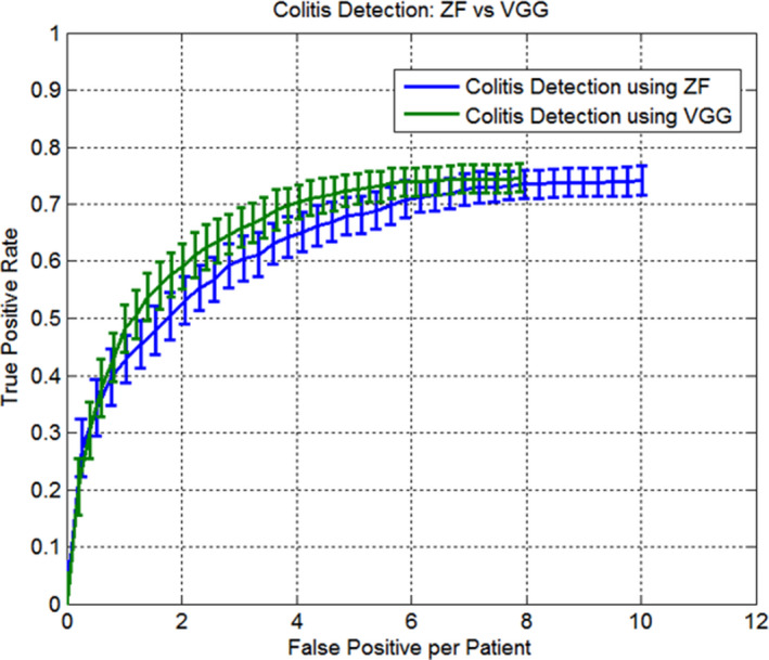
Average FROC of colitis detection of using ZF net and VGG net. The maximal TPR for ZF and VGG are 73.9% and 74.8%, respectively. [Color figure can be viewed at wileyonlinelibrary.com]
For patient‐level colitis diagnosis, Fig. 14 shows that Faster RCNN with VGG net slightly outperformed Faster RCNN with ZF net, increasing AUC from 0.984 ± 0.008 to 0.986 ± 0.007 (P = 0.4). The sensitivity is 93.7% (75.0/80) and the specificity is 95.0% (76.0/80) at the optimal operating point for the Faster RCNN with VGG net.
Figure 14.

Patient‐level diagnosis ROC curves of ZF net and VGG net. [Color figure can be viewed at wileyonlinelibrary.com]
Colitis diagnosis with CNNs significantly outperformed the method with hand‐crafted features,15 which reported AUC of 0.75, sensitivity of 72.7% and specificity of 73.3% in a small dataset. All results about colitis detection and diagnosis are summarized in Table 2. Since both RCNN and VGG net are computationally expensive, we only evaluated the Faster RCNN with VGG net.
Table 2.
Summarized colitis detection and diagnosis results
| Method | Detection | Diagnosis | |||
|---|---|---|---|---|---|
| mAP | Sensitivity at 2 FPs/patient | AUC | Sensitivity at the operating point | Specificity at the operating point | |
| RCNN with ZF net | 48.7% | 51.4% | 0.978 ± 0.009 | 90.4% (72.3/80) | 94.0% (75.2/80) |
| Faster RCNN with ZF net | 50.9% | 54.0% | 0.984 ± 0.008 | 91.6% (73.3/80) | 95.0% (76.0/80) |
| Faster RCNN with VGG net | 56.9% | 58.4% | 0.986 ± 0.007 | 93.7% (75.0/80) | 95.0% (76.0/80) |
| Codebook with Gabor filters15 | – | – | 0.750 | 72.7% (16/22) | 73.3% (11/15) |
4.D. Computation time
The colitis detection and diagnosis are implemented based on the RCNN (https://github.com/rbgirshick/rcnn) and Faster RCNN (https://github.com/ShaoqingRen/faster_rcnn) with Matlab 2014. Our code for colitis detection is online available. (https://github.com/rsummers11/CADLab)
For the colitis detection using RCNN with ZF net, the training on 60 patients and 60 normal cases on a TITAN Z GPU took around 10 h for each fold. For the colitis detection using Faster RCNN, for each fold, the single‐stage training time reduced to 2.5 h for ZF net and 4 h for VGG net, respectively.
Once we trained the net, testing was very fast and nearly real time for Faster RCNN. The test times are shown in Table 3.
Table 3.
Test Time (ms) on a TITAN Z GPU
| Method | # Proposals | Time (ms) |
|---|---|---|
| RCNN with ZF net | 3000 | 2600 |
| Faster RCNN with ZF net | 300 | 60 |
| Faster RCNN with VGG net | 300 | 200 |
4.E. Visualizing learned features
We demonstrate the learned features for colitis detection by retrieving the images that maximally activate a neuron in the CNNs.18 The idea is to let the selected feature “speak for itself” by showing which inputs it fires on. Features from the fifth pool layer of ZF net are visualized. Each group in Fig. 15 displays the top 24 activations (including receptive fields and activation values) for one pool5 feature from a CNN of ZF net for colitis detection. These five features were selected to display the representative samples of the CNN learns. The first feature represents the thickened colon wall of colitis. The second feature represents the accordion appearance of colitis. The third, fourth, and fifth features represent the appearance of normal colon, vertebra, and kidneys respectively. These rich features are crucial for accurate colitis detection.
Figure 15.

Top 24 region proposals (including the receptive fields and activation values) for five pool5 features. A red box surrounds each of the five feature groups. Feature 1 captured the thickened colon wall of colitis. Feature 2 captured the accordion appearance of colitis. The appearances of normal colon, vertebra, and kidney were captured in features 3, 4, and 5, respectively. [Color figure can be viewed at wileyonlinelibrary.com]
5. Discussion
The abdominal region exhibits great complexity on CT, and this is exemplified by the path of the colon. For example, the course of the colon through the abdomen is tortuous. Its position, length, contents, and distension vary greatly among different patients and even on serial scans of the same patient.27, 28 Consequently, detecting colitis regions is a difficult task.
A number of papers have described the radiologic features of colitis on CT. Johnson et al.29 showed the usefulness of CT for detecting colitis and other IBDs. Balthazar et al.30 studied 54 cases with proven ischemic colitis and presented the CT clinical findings and assessed the effects of treatment. Thoeni and Cello31 showed different types of colitis and described the key clinical aspects, imaging findings, and differential diagnosis of each type. However, these works all depended on manual assessment of the images by a radiologist. Compared to these manual methods, our method can automatically identify colitis potentially greatly simplifying the task of colitis detection for the radiologist.
Designing features that describe an object is crucial in a computer‐aided detection task. Compared to the hand‐crafted features, CNNs learn deep features by a training procedure. Figure 15 shows the learned features by retrieving the images that maximally activate a neuron in the CNNs. The indicators of colitis, the thickened colon wall, and the accordion sign, were successfully learned by CNNs. The appearance of normal colon, vertebra, and kidneys were also learned by CNNs.
The results in Table 2 show that the lesion‐based colitis detection reported a relative lower performance (mean mAP of 52.2%) compared to the patient‐level colitis diagnosis (mean sensitivity of 91.9%). However, colitis is a regional disease, not a focal lesion like a polyp or a tumor. So patient‐level diagnostic performance is more clinically important than the lesion‐level detection performance. With the correct diagnosis, treatment of colitis is aimed at eliminating the underlying cause of the inflammatory process, resting the inflamed bowel, and restoring the nutritional status to normal. Consequently, our method's high patient‐level sensitivity and specificity are encouraging for potential clinical use.
Table 2 also demonstrates that the colitis detection and diagnosis using Faster RCNN with VGG net performs best. One reason is the RPN in the Faster RCNN generates fewer (300) but higher quality region proposals, compared to the region proposals (3000) output by selective search in the RCNN. In addition, the neurons of the deeper VGG net have larger receptive fields to capture more context information to improve detection performance.
One limitation of this work is the method detected colitis mainly on the basis of increased colonic wall thickness and “accordion” appearance in 2D view. Therefore, without any prior anatomical knowledge, some normal organs with similar appearance, such as stomach or gallbladder, could be classified as colitis. To remove detections on extracolonic anatomy, it may be possible to incorporate anatomic knowledge of colon location using vascular and probabilistic features.32 Another limitation is the normal patients had higher resolution images than the colitis patients (1.5–2.5 mm vs. 3–5 mm slice thickness), which may lead to the good specificity for colitis diagnosis.
Finally, our method may have future beneficial application to other diseases that manifest with bowel wall thickening such as colorectal cancer, inflammatory bowel disease, diverticular disease, and diverticulitis, although this would need to be validated.
6. Conclusion
In this work, we demonstrate that the CNN pretrained on ImageNet could be adopted for colitis detection on CT images. The Faster RCNN architecture allowed convolution layers to be shared by the region proposal network and the detection network for a unified approach. Compared to our previous approach using RCNN, the Faster RCNN method yielded better performance with markedly reduced runtime for both training and testing. With the use of VGG net for the Faster CNN, we obtained high sensitivity (93.7%) and specificity (95.0%) showing that this method has strong potential as a clinical tool for use in colitis screening.
Conflict of interest
Regarding disclosures, author Summers has pending and/or awarded patents for related automated analyses for CT colonography. Author Summers receives royalty income for a patent license from iCAD and software licenses to Imbio and Zebra Medical. Author Summers’ laboratory receives research support from Ping An Technology Company Ltd. All other authors have no conflicts of interest.
Acknowledgments
This research was supported by the Intramural Research Program of the NIH Clinical Center. The mention of commercial products, their sources, or their use in connection with material reported herein is not to be construed as either an actual or implied endorsement of such products by the Department of Health and Human Services.
References
- 1. Samadder NJ, Gornick M, Everett J, Greenson JK, Gruber SB. Inflammatory bowel disease and familial adenomatous polyposis. J Crohns Colitis. 2013;7:e103–e107. [DOI] [PubMed] [Google Scholar]
- 2. Fisher JK. Abnormal colonic wall thickening on computed tomography. J Comput Assist Tomogr. 1983;7:90–97. [DOI] [PubMed] [Google Scholar]
- 3. Fichtner‐Feigl S, Kesselring R, Strober W. Chronic inflammation and the development of malignancy in the GI tract. Trends Immunol. 2015;36:451–459. [DOI] [PMC free article] [PubMed] [Google Scholar]
- 4. Cutinha AH, De Nazareth AG, Alla VM, Bewtra A. Clues to colitis: tracking the prints. West J Emerg Med. 2010;11:112–113. [PMC free article] [PubMed] [Google Scholar]
- 5. Macari M, Balthazar EJ, Megibow AJ. The accordion sign at CT: a nonspecific finding in patients with colonic edema. Radiology. 1999;211:743–746. [DOI] [PubMed] [Google Scholar]
- 6. Kirkpatrick IDC, Greenberg HM. Evaluating the CT diagnosis of clostridium difficile colitis: should CT guide therapy? Am J Roentgenol. 2001;176:635–639. [DOI] [PubMed] [Google Scholar]
- 7. Ren S, He K, Girshick R, Sun J. Faster R‐CNN: towards real‐time object detection with region proposal networks. IEEE Trans Pattern Anal Mach Intell 2016;39:1137–1149. [DOI] [PubMed] [Google Scholar]
- 8. Dalal N, Triggs B. Histograms of oriented gradients for human detection. 2005 IEEE Computer Society Conference on Computer Vision and Pattern Recognition, Vol 1, Proceedings; 2005: 886–893.
- 9. Lowe DG. Distinctive image features from scale‐invariant keypoints. Int J Comput Vision. 2004;60:91–110. [Google Scholar]
- 10. Greenspan H, van Ginneken B, Summers RM. Deep learning in medical imaging: overview and future promise of an exciting new technique. IEEE Trans Med Imaging. 2016;35:1153–1159. [Google Scholar]
- 11. Roth HR, Lu L, Seff A, et al. A new 2.5D representation for lymph node detection using random sets of deep convolutional neural network observations. Med Image Comput Comput Assist Interv. 2014;17:520–527. [DOI] [PMC free article] [PubMed] [Google Scholar]
- 12. Qi D, Hao C, Lequan Y, et al. Automatic detection of cerebral microbleeds from MR images via 3D convolutional neural networks. IEEE Trans Med Imaging. 2016;35:1182–1195. [DOI] [PubMed] [Google Scholar]
- 13. Ghesu FC, Krubasik E, Georgescu B, et al. Marginal space deep learning: efficient architecture for volumetric image parsing. IEEE Trans Med Imaging. 2016;35:1217–1228. [DOI] [PubMed] [Google Scholar]
- 14. Brosch T, Tang LY, Youngjin Y, Li DK, Traboulsee A, Tam R. Deep 3D convolutional encoder networks with shortcuts for multiscale feature integration applied to multiple sclerosis lesion segmentation . IEEE Trans Med Imaging. 2016;35:1229–1239. [DOI] [PubMed] [Google Scholar]
- 15. Wei ZS, Zhang WD, Liu JF, Wang SJ, Yao JH, Summers RM. Computer‐aided detection of colitis on computed tomography using a visual codebook. IEEE 10th Int Symp Biomed Imaging. 2013;2013:141–144. [Google Scholar]
- 16. Liu J, Wang D, Wei Z, et al. Colitis detection on computed tomography using regional convolutional neural network. In International Symposium on Biomedical Imaging; 2016.
- 17. Uijlings JRR, van de Sande KEA, Gevers T, Smeulders AWM. Selective search for object recognition. Int J Comput Vis. 2013;104:154–171. [Google Scholar]
- 18. Girshick R, Donahue J, Darrell T, Malik J. Rich feature hierarchies for accurate object detection and semantic segmentation. IEEE Conf Comput Vis Pattern Recognit (Cvpr). 2014;2014:580–587. [Google Scholar]
- 19. Alexe B, Deselaers T, Ferrari V. Measuring the objectness of image windows. IEEE Trans Pattern Anal Mach Intell. 2012;34:2189–2202. [DOI] [PubMed] [Google Scholar]
- 20. Carreira J, Sminchisescu C. CPMC: automatic object segmentation using constrained parametric min‐cuts. IEEE Trans Pattern Anal Mach Intell. 2012;34:1312–1328. [DOI] [PubMed] [Google Scholar]
- 21. Jia Y, Shelhamer E, Donahue J, et al. Caffe: Convolutional Architecture for Fast Feature Embedding. arXiv preprint arXiv:1408.5093; 2014.
- 22. Zeiler MD, Fergus R. Visualizing and understanding convolutional networks. Comput. Vis. ‐ Eccv 2014, Pt I. 2014;8689:818–833. [Google Scholar]
- 23. Girshick R. Fast R‐CNN. IEEE Int Conf Comput Vis (ICCV). 2015;2015:1440–1448. [Google Scholar]
- 24. Achanta R, Shaji A, Smith K, Lucchi A, Fua P, Susstrunk S. SLIC superpixels compared to state‐of‐the‐art superpixel methods. IEEE Trans Pattern Anal Mach Intell. 2012;34:2274–2282. [DOI] [PubMed] [Google Scholar]
- 25. Chakraborty DP. Recent advances in observer performance methodology: jackknife free‐response ROC (JAFROC). Radiat Prot Dosimetry. 2005;114:26–31. [DOI] [PubMed] [Google Scholar]
- 26. Simonyan K, Zisserman A. Very Deep convolutional networks for large‐scale image recognition. In ICLR2015; 2015.
- 27. Eickhoff A, Pickhardt PJ, Hartmann D, Riemann JF. Colon anatomy based on CT colonography and fluoroscopy: impact on looping, straightening and ancillary manoeuvres in colonoscopy. Dig Liver Dis. 2010;42:291–296. [DOI] [PubMed] [Google Scholar]
- 28. Hanson ME, Pickhardt PJ, Kim DH, Pfau PR. Anatomic Factors predictive of incomplete colonoscopy based on findings at CT colonography. Am J Roentgenol. 2007;189:774–779. [DOI] [PubMed] [Google Scholar]
- 29. Johnson KT, Hara AK, Johnson CD. Evaluation of colitis: usefulness of CT enterography technique. Emerg Radiol. 2009;16:277–282. [DOI] [PubMed] [Google Scholar]
- 30. Balthazar EJ, Yen BC, Gordon RB. Ischemic colitis: CT evaluation of 54 cases. Radiology. 1999;211:381–388. [DOI] [PubMed] [Google Scholar]
- 31. Thoeni RF, Cello JP. CT imaging of colitis. Radiology. 2006;240:623–638. [DOI] [PubMed] [Google Scholar]
- 32. Zhang WD, Liu JM, Yao JH, Summers RM. Reducing False Positives of Small Bowel Segmentation on CT Scans by Localizing Colon Regions. Medical Imaging 2014: Computer‐Aided Diagnosis, 9035; 2014.