Abstract
Location uncertainty has been a major barrier in information mining from location data. Although the development of electronic and telecommunication equipment has led to an increased amount and refined resolution of data about individuals’ spatio-temporal trajectories, the potential of such data, especially in the context of environmental health studies, has not been fully realized due to the lack of methodology that addresses location uncertainties. This article describes a methodological framework for deriving information about people’s continuous activities from individual-collected Global Positioning System (GPS) data, which is vital for a variety of environmental health studies. This framework is composed of two major methods that address critical issues at different stages of GPS data processing: (1) a fuzzy classification method for distinguishing activity patterns; and (2) a scale-adaptive method for refining activity locations and outdoor/indoor environments. Evaluation of this framework based on smartphone-collected GPS data indicates that it is robust to location errors and is able to generate useful information about individuals’ life trajectories.
Keywords: GIS, Data Mining, Fuzzy Logic, GPS, Scale Space, Spatial Uncertainty
1. Introduction
The association between location-specific characteristics (e.g., neighborhood context, built environment, environmental exposure) and health has long been recognized in the fields of environmental health and human-environment interactions (Kwan 2000, Richardson et al. 2013). Researchers often use individuals’ locations to extract contextual indicators about social and natural environments, which are then associated with health outcomes. Traditionally, the location data for such studies was either based on residential addresses or obtained from a questionnaire survey. These data sources tend to be inaccurate and unable to capture the continuous life trajectory of an individual (Bowling 2005, Schenk et al. 2011). The development of location-measurement equipment such as GPS units, which come with increased accuracy and enhanced portability, has made it possible to record individuals’ locations and movements more precisely and continuously. The passive data collection of GPS units also greatly relieves human subjects from labor- and attention-intensive procedures of surveys and questionnaires (Schenk et al. 2011; Chen, Bian, and Ma 2014). The advantages of GPS-based location measurement have not only benefited traditional location-health studies, but have also increased the variety of new environment-health investigations in recent years (Elgethun et al. 2007, Cooper et al. 2010, Wheeler et al. 2010, Wu et al. 2011, Hirsch et al. 2014, Jankowska, Schipperijn, and Kerr 2015, Steinle et al. 2015).
More recently, the smartphone has emerged as a new location measurement tool in health studies (Wiehe et al. 2008, Montoliu and Gatica-Perez 2010, Tung et al. 2011, Carlson et al. 2012). Smartphones not only record GPS points at comparable location accuracy to traditional GPS-enabled units (Wiehe et al. 2008, Wan et al. 2013), but also provide functions such as real-time data transfer, communication, and acceleration monitoring that are not available on traditional GPS units. The increasing popularity of smartphones also makes it possible to implement studies within large populations while minimizing participants’ data–collection burden. Considering these factors, smartphones represent a future trend for location measurement in health studies.
Although the use of GPS units in health-related studies has increased, researchers lack efficient methods to extract health-related activity information accurately from GPS traces (Thierry, Chaix, and Kestens 2013, Wan et al. 2013). Activity-specific characteristics are vital for correctly evaluating environment-health relationships. For example, accurate information on subjects’ indoor/outdoor status and the corresponding duration is needed for environmental exposure evaluation (Elgethun et al. 2007, Whyatt et al. 2007, Wu et al. 2011). Physicians also need data on a patient’s walking duration, gait speed, and life-space to evaluate his/her functional status (Herrmann et al. 2011, Schenk et al. 2011). Previous GPS processing protocols were primarily designed for transportation studies and are not suitable for dealing with person-collected GPS data. Compared to transportation GPS data, which are captured primarily by vehicle-equipped GPS units that have satisfactory location accuracy, person-collected GPS points are more likely to be inaccurate and to suffer data loss due to satellite signal shielding and battery depletion. These limitations pose extra challenges for GPS data processing, pointing to the need to develop new or improved methodology that can account for different levels of location inaccuracy and inconsistent data recording. Although traditional spatial methods such as point clustering analysis have the potential to overcome the methodological limitations, they have not been fully adapted to account for the spatio-temporal features of GPS data.
To solve these challenges, this article presents an integrated framework of GPS data classification that can accurately derive individuals’ activity characteristics while accounting for data uncertainties. Taking advantage of the fuzzy logic theory and the scale-space theory, this framework incorporates both the attributes of single points and the spatial pattern of point clusters to infer accurate and detailed information about human activities that is suitable for environment-health studies. The remainder of this article is organized as follows. We first review current methods of GPS-based activity identification, point clustering analysis, as well as the scale-space theory, and identify the need for developing new methods to overcome current limitations. A fuzzy classification method and a scale-adaptive method are then introduced to address the need, followed by an evaluation of these methods based on a set of smartphone GPS data. The discussion section demonstrates the fundamental contribution of the proposed methods to GIScience and their wide applicability in environment-health studies.
2. Related Work
The primary purpose of GPS data classification in environment-health studies is to derive activity-specific information such as location, duration, environmental context, and trip purposes that is vital for inferring health behaviors and environmental exposures. For this purpose, the raw GPS data first undergoes a preliminary classification to derive human activity patterns such as staying, walking, and other transportation. Then, points of staying activities go through further processing to infer detailed information (e.g., true location, indoor/outdoor, duration). Various methods, including activity pattern identification methods, point cluster analysis, and scale-space methods, have the potential to accomplish these two steps.
GPS-based activity pattern identification
Methods of GPS-based activity pattern identification generally follow a segmentation procedure (Ashbrook and Starner 2003, Liao, Fox, and Kautz 2007, Guc et al. 2008, Zheng et al. 2008, Zhang et al. 2011, Schuseeler and Axhausen 2008). These methods first determine a set of change points based on point characteristics such as speed and acceleration. These change points divide the whole GPS stream into connected segments. Then, an activity status (e.g., walking, driving) is inferred for each segment. The determination of change points is implemented by using either rule-based or inference-based models. Rule-based models use some simple or hybrid rules to distinguish coarse statuses (Schuseeler and Axhausen 2008, Wan and Lin 2013). Although rule-based models are straightforward and easy to implement, they adopt uniform parameters for different individuals, which tends to be inaccurate. Instead of using the one-for-all threshold values, inference-based models adopt learning procedures to estimate individual-specific parameters for the classification (Liao et al. 2007; Zheng et al. 2008; Zhang et al. 2011). The fuzzy classification method described in this study benefits from the idea of the inference method, but incorporates a way to handle a non-linear relationship between individual-collected GPS data and activity patterns.
Point cluster analysis
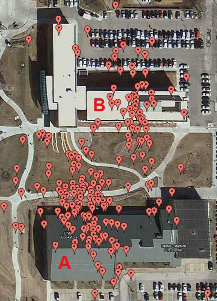
The activity pattern identification described above derives only coarse categories of human activities such as walking, staying, and driving. To infer more detailed information on staying activities such as location(s), trip purpose, contextual environment, and duration, GPS points that are classified as staying activities must be further processed. For example, two staying activities with a short time gap may be identified as one staying activity at preliminary classification (Figure 1). In this case, the two activities may exhibit as two sub-locations of the combined activity and need to be distinguished at subsequent analyses. The preliminary classification is also inadequate for inferring trip purposes or indoor/outdoor environments. It is also widely accepted that a single GPS point cannot be used to determine the exact activity location, which should be inferred based on the spatial pattern of points (Wan et al. 2013, Thierry, Chaix, and Kestens 2013). Cluster methods provide a potential solution to this type of uncertainty.
Figure 1.
An example of mixed staying activities reflected by smartphone collected GPS points. In this figure, the subject first stayed inside building A before going to building B. However, the inaccuracy of GPS points made it difficult to distinguish the two sub-locations and to derive contextual information (e.g., inside or outside a building) about the subject’s activities.
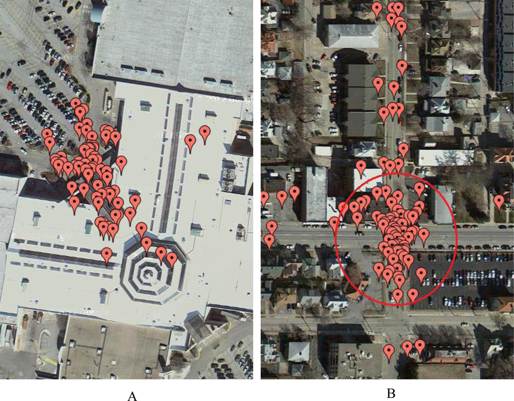
Point cluster analysis has long been a topic in the fields of GIScience, computer science, and electronic engineering and has been widely applied in environment-health studies to explore disease patterns. One important branch of point cluster methods focuses on data mining or machine learning from point groups, without controlling for background factors such as population density (Ester et al. 1996, Ankerst et al. 1999, Kaufman and Rousseeuw 1990, Ng and Han 1994,). These methods have proved effective in detecting clustering of points. However, they are not directly applicable for discovering the structure of GPS points, which include both spatial attributes and temporal characteristics. The structure of GPS points should be characterized by spatio-temporal clusters rather than by purely spatial clusters. In this article, a spatio-temporal cluster of GPS points is defined as a group of GPS points which exhibit both spatial clustering and temporal continuity. Figure 2 shows an example of the differences between a spatial cluster and a spatio-temporal cluster. Points in Figures 2a and 2b both exhibit a spatial clustering trend. However, only Figure 2A shows spatio-temporal clustering because the points are both spatially clustered and temporally connected. Temporal connection requires incorporating time information into cluster analysis of GPS points.
Figure 2.
Examples of spatio-temporal cluster (A) and spatio-non-temporal cluster (B). The spatio-temporal cluster shown in (A) reflects a staying activity for which the GPS points were sequentially observed (Note: this is an activity where a subject stayed inside a building for 35 minutes. The subject spent most of the time close to the entrance of the building. The GPS points exhibit a cluster regardless of the temporal sequence). The spatio-non-temporal cluster noted in the red circle in (B) is composed of GPS points that were observed during multiple days when the subject drove past the road intersection. The latter is categorized as a spatio-non-temporal cluster because the GPS points were not sequentially observed and therefore do not fulfill the temporal continuity criterion.
Scale space theory
Scale space theory is a theoretical framework for multi-scale representation of natural or social phenomena (Witkin 1983;Koenderink 1984; Lindeberg 1993, Lindeberg 1998). It represents a branch of the broader field of scale studies which deal with phenomena representation in multiple disciplines such as geography, physics, and computer science. The notion of scale space was inspired by the unique characteristic of scale: a phenomenon can be perceived in different ways with the change of scale, as local details gradually disappear or merge into new features when the scale transitions from fine to coarse. By monitoring this change, important features can be discovered that are not necessarily reflected by a single-scale representation, and an optimal scale can be determined that best exhibits a pattern of interest (Lindeberg 1998). Multi-scale representation allows researchers to explore the structure of the phenomenon and to capture features of interest such as local clusters. These advantages have made scale space widely applicable in fields such as computer science and geography to understand and explore spatial and non-spatial patterns (Lindeberg 1993, Mu and Wang 2008).
In general, a scale space representation of a phenomenon (or image) I(x,y) is expressed as
| (1) |
where S(σ) represents a Gaussian smoothing process, with σ being the smoothing parameter. The scale space of this image can be constructed as a group of gradually increased σ (i.e., the level of smoothing) and the corresponding smoothed images.
The two major advantages of scale space methods are that they can be used to identify both local features and the overall structure and that they rely less on priori knowledge of the probability distribution of events than do model-based methods. These advantages have inspired researchers to incorporate scale space methods into various spatial clustering methods, especially hierarchical methods (Leung, Zhang, and Xu 2000, Luo, Zhou, and Leung 2002, Wong and Posner 1993, Ciucu et al. 2003; Mu and Wang 2008). Although sharing the same theoretical background, these methods are generally implemented differently. For example, by simulating how human eyes capture the structure of a scene, blurring algorithms have been developed to detect significant features and to remove disturbing features within a scene (Leung, Zhang, and Xu 2000; Luo et al. 2002). In general, a phenomenon or scene is processed as an image, and the human lateral retina recognizes the phenomenon structure based on pixel brightness or color. As the distance between the individual and the scene gradually increases, the image gets blurred in the retina. In this case, the distance behaves as the scale parameter. By applying the principles of thermodynamics, Wong et al. (1993) developed a melting algorithm to classify crop types from a synthetic aperture radar image (Wong 1993; Ciucu et al. 2003). In this algorithm, the effect of scale is represented by a temperature parameter T, which could be interpreted as the inverse of σ in formula 1. The hierarchical clustering structure is captured by simulating the melting process caused by increased temperature, and a cluster center is detected as the local maximum of information entropy based on pixel values.
Based on the blurring and the melting algorithms, Luo et al. (2002) and Mu and Wang (2008) further extended raster-based scale-space clustering methods to analyze vector data. Different from regularly arrayed pixels in raster processing, vector data is characterized by irregularly grouped polygons (e.g., census tracts) within a two-dimensional space. To address this challenge, Mu and Wang (2008) used attribute distance to measure the similarity of adjacent polygons and melt each polygon into the neighbor with the shortest attribute distance. By doing this, both spatial proximity and attribute homogeneity are accounted for during polygon melting. In Mu and Wang (2008), each round of melting leads to more aggregated (and fewer) polygons, which mimics the scale-space blurring process. By reducing neighbor-homogeneity, vector-based scale-space methods have great applicability in addressing the methodological limitations of social studies, such as the small number problem, the modifiable area unit problem, and limitations brought about by spatial autocorrelations.
The advantages of scale-space theory make it applicable for exploring meaningful information about staying activities from GPS points. For example, in the case of multiple sub-locations (i.e., the subject stayed in several locations, or sub-locations, during a detected staying activity) in Figure 1, the point density will exhibit several clusters at specific levels of smoothing that correspond to the sub-locations. Sub-locations can be extracted to represent the two indoor activities at an appropriate level of scale. However, these advantages received little attention in the cluster detection domain. In addition, similar to point clustering methods, current scale-space clustering methods are unable to adjust for the temporal information, which poses a further challenge for the implementation.
3. Methodology Development
The methodology presented in this article is an integrated scheme that enhances the two basic steps of GPS-based activity classification: a fuzzy classification method for differentiating activity patterns and a scale-adaptive method for inferring activity locations. The fuzzy classification method derives coarse categories of an individual’s continuous activities. Then, the scale-adaptive method further refines the location(s) of staying activities to identify trip purposes and distinguish indoor/outdoor environments.
3.1 Fuzzy classification of GPS points
Before describing the fuzzy classification method, we first explain the concept of activities in GPS data processing. Activities could be defined as behaviors that individuals take to fulfill specific purposes. Following Wan and Lin (2016), this study groups an individual’s everyday activities into three statuses that could be well represented by GPS data: staying, walking, and other transportation. A detailed explanation and justification of these activity types is provided in Table 1. Table 1 also lists and explains other terms of this paper.
Table 1.
Explanations of terms used in this article
| Term | Meaning |
|---|---|
| Activity Types for
Fuzzy Classification |
|
| Walking* | Walking activities are those when an individual walks outdoors. |
| Staying | Staying activities are those performed when an
individual stays at or around a location, such as shopping, staying at home, indoor walking, and dining out. |
| Other Transportation | Other transportation activities include other
motorized or non- motorized transportation such as driving a car, bus riding, and cycling. |
| Baseline Activities | Baseline activities are the group of
activities that 1) were recorded by the three subjects in journals and confirmed/corrected by the subsequent GIS validation and 2) that were not recorded by the journals but identified by the subject during the GIS validation. Information of baseline activities serves as the reference for evaluating the performance of the two methods developed in this study. |
| Membership Function | In fuzzy logic methods, membership functions
are defined as the function that projects an input crispy value into a membership degree that ranges between 0 and 1. |
| Spatio-temporal cluster | In this article, a spatio-temporal cluster of
GPS points is defined as a group of GPS points which exhibit both spatial clustering and temporal continuity. |
| Sub-location | During a staying activity, the subject may
actually stayed at several locations (for example, a subject’s staying at home activity may include sub-locations in the living-room and the yard) within the geographic range. Correspondingly, GPS points of the staying activity may exhibit several spatio-temporal clusters which denotes these sub- locations. |
The reason why we emphasize outdoor for walking activities is that when an individual walks inside a building (for example, walking inside a gym, shopping at Walmart), the GPS points may still exhibit a cluster around the building location, which makes it difficult for algorithms to distinguish. Therefore, indoor walking would be categorized into staying activities.
Conventional GPS data classification relies on the characteristics of single points, which tend to be inaccurate due to GPS errors. The influence and homogeneity of neighboring points has seldom been used to refine the inaccuracy of single point characteristics. Fuzzy logic, a type of reasoning theory that deals with ambiguous data, could help solve this problem. A major advantage of fuzzy classification methods is that they can process approximate input values, which makes them suitable for processing inaccurate GPS points. Wan and Lin (2016) developed a fuzzy classification and aggregation method to address uncertainties of point location inaccuracy and to account for the non-linear relationship between GPS data and activity patterns. This current study will primarily follow the method in Wan and Lin (2016) to identify activity patterns.
A fuzzy classification method is composed of three steps: input fuzzification, fuzzy inference, and output estimation (Mamdani and Assilian 1975, Takagi and Sugeno 1985). The input fuzzification uses predefined functions to transform crisp input values (e.g., quantitative numbers) into descriptive terms (e.g., qualitative values) that are suitable for fuzzy inference. For example, in terms of an individual’s motion status, a speed of 2 m/s (i.e., a crisp value) could be fuzzified into probabilities for descriptive terms such as fast, slow, and zero. The fuzzy inference then uses a set of pre-defined rules to infer the likelihood of each output variable. One example of the inference rules is “if the speed is zero, then the probability of staying is high.” In this case, the output variable is “staying” and the corresponding probability is “high.” Last, the descriptive output terms (e.g., “high” in the inference example) are defuzzified into crisp values (e.g., 90 percent probability of staying). A thorough explanation of the fuzzy classification of GPS points could be found in Wan and Lin (2016).
In this study, the selections of input variables, fuzzification functions, and the fuzzy inference follow those of Wan and Lin (2016). Specifically, we used two GPS point indicators, point speed and point angle, as input variables. Since we are interested in three outcomes (i.e., walking, staying, and other transportation), three inference systems were adopted, each focusing on one outcome. For each inference engine, the inference and the output estimation generated a probability for the specific outcome (i.e., walking, staying, and other transportation). The output variable with the largest probability was then selected as the preliminary status of the point. After all points were assigned a status, a segment-aggregation strategy (Wan and Lin 2016) was adopted to generate continuous segments that represent the classified activities.
3.2 A scale-adaptive clustering method for inferring activity locations
Overall strategy of the scale adaptive method
As revealed in Figure 1, staying activities derived by fuzzy classification may contain several sub-locations that cannot be differentiated by point speed or point angle. The lack of such information may impede investigation into topics such as exposure modeling (Wu et al. 2011) and functional status assessment (Schenk et al. 2011). In this section, a scale-adaptive method is developed to identify these sub-locations. Rooted in the scale-space theory, hierarchical clustering methods, and density clustering methods, this proposed method adopts an iterative strategy to explore the spatio-temporal structure of GPS points within a staying activity. The spatio-temporal structure is then used to estimate sub-locations. The overall strategy is composed of several major steps:
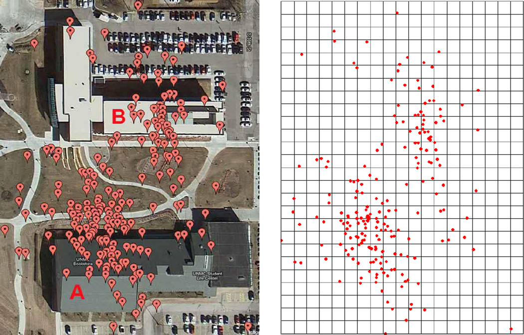
Rasterize the covering area of the GPS points, Da, of a staying activity by dividing the area into regular square cells with a pre-defined size (e.g., 7 meters). The rasterized cells along with the original GPS points (shown in Figure 3) will serve as the major inputs for subsequent calculation. Define a Gaussian function and set the Gaussian smoothing parameter σ to 0.
- Increase σ by 1 and calculate the density of each cell (i, j) by
Where dk,i,j is the distance between the cell center and point k, and G(d, σ) is the Gaussian function . Gaussian function is considered the best filter for image smoothing in scale-space studies because of its advantage in avoiding creating new spurious structure at coarse scales (Babaud et al. 1986; Yuille and Poggio 1986; Lindeberg 1990). Use a spatio-temporal criterion to find all clusters within the covering area, and record them in a new layer. The details of the spatio-temporal criterion will be described later.
For each identified spatio-temporal cluster, determine its affiliation status by linking it to clusters of the previous layer. The determination of affiliation status will be illustrated in a subsequent section.
Repeat steps 2, 3, and 4. The iteration continues until all clusters stop growing. The result of the iteration will be a pyramid-shaped structure that contains clusters detected at different levels, with the bottom level being the first layer of clusters and the top level being the level at which the iteration stops.
Figure 3.
Original GPS points and rasterized cells (cell size = 7 meters) for the staying activity in Figure 1.
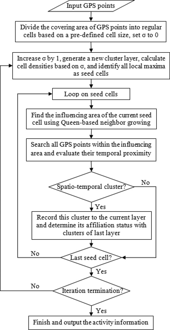
The above-mentioned steps ensure that all sub-locations within the same staying activity can be identified and indexed in a bottom-up structure. These steps are illustrated in the flow chart in Figure 4. Below we will use GPS points in Figure 1 to explain how each step works.
Figure 4.
Flow chart of the scale-adaptive clustering method (Note: this flow chart does not contain procedures of the fuzzy classification method developed in this study)
Spatio-temporal cluster identification
Correct identification of spatio-temporal clusters to represent sub-locations of a staying activity is the key to the proposed scale-adaptive method. Our conceptual criterion for a spatio-temporal cluster is that the GPS points containing the cluster should be spatially clustered, and temporally connected. We designed a two-step procedure to address the spatial and temporal requirements. In the first step, the spatial clustering of cells was determined using a seed-growing strategy. Specifically, cells with local maxima (i.e., those whose density value is larger than their neighbors) of density were first selected as seed cells. The influencing region of each seed cell was then constructed by expanding it to neighbor cells. During the expansion, if any neighbor of a cell within the influencing region had a smaller density value than the current cell, then this neighbor cell was added to the region. To avoid including zero-value cells in the expansion, we excluded cells whose density was significantly lower than the average density of all cells. Borrowing the concept of significance from statistics, we defined the exclusion threshold to be 0.05 times the average density. Therefore, the expansion only applied to cells whose density was higher than 0.05 times the average density of all cells. The expansion continued until all boundary cells of the influencing region had a smaller density value than their out-of-region neighbors. Queen topology was employed during the seed growing. Unlike Rook topology, which links only neighboring cells that have common boundaries, Queen topology links both those that have common boundaries and those that have common vertexes. This characteristic of the Queen-based expansion makes it possible to reach all neighboring cells and avoid missed cells during the expansion. Following traditional literature, we call the final influencing region of each local maxima a ‘spatial cluster’.
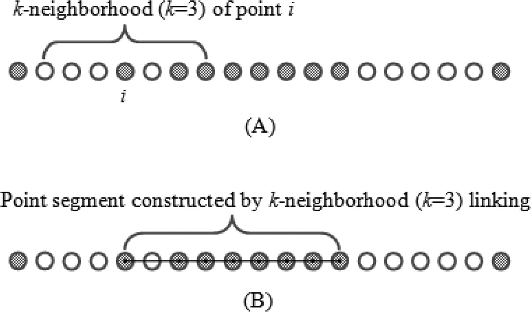
After the whole cover area has been decomposed into one or more spatial clusters, the second step identifies spatio-temporal clusters from the spatial clusters. For each spatial cluster, all GPS points within it are sorted according to their observational time, and their temporal continuity is checked. Due to the existence of point outliers (e.g., points that deviate greatly from the true location), it may not be appropriate to use the time difference between the first point and the last point to represent the duration of a spatial cluster. In addition, points that are recorded between the first and last points but are not included in the cluster may introduce further uncertainties. To address these challenges, we introduced a modified point aggregation process to assess point continuity within a spatial cluster and to identify ‘true’ starting and ending points for it. This approach is based on the definition of k-neighborhood, a concept that is commonly used in density-based clustering methods (Ester et al. 1996, Ankerst et al. 1999, Duan et al. 2007). In general, the k-neighborhood of a point, p, is defined as the collection of points that are within the k Euclidean distance from p. In this article, we modified the definition by changing Euclidean distance to sequential distance: the k-neighborhood of p was defined as the collection of points whose observational sequence in the original GPS dataset was less than k units from that of p. In practice, if two sequentially observed points in the cluster are within the k-neighborhood of each other, then these two points are considered k-neighbors and are linked. After the linking process is finished for all pairs of sequential points within the cluster, one can identify several segments that are composed of linked points. The processes of k-neighborhood linking and segment construction are illustrated in Figure 5. The duration of a linked point segment could be calculated as the time difference between the first and the last point of the segment. After the segments were determined, we defined a spatio-temporal cluster as a spatial cluster in which there was at least one segment with a duration longer than a threshold value (e.g., 300 seconds). All of these long-duration segments were selected and recorded to represent this current spatio-temporal cluster. Note that due to point deviations, there were still time gaps between the selected segments (if there are more than one long-duration segments). These gaps will be gradually filled during the cluster aggregation process which will be described in the next section. The duration of the spatio-temporal cluster was therefore represented by the time gap between the first point of the first segment and the last point of the last segment.
Figure 5.
Definition of k-neighborhood (A) and linked point segment (B). The dots represent sequentially observed GPS points, with the dark dots being those within the same spatial cluster and the white dots being outside of the cluster. Note that the spatial location information of each point was removed so that they were ranked by the temporal sequence only.
The k-neighborhood aggregation allowed us to examine the temporal continuity of points while excluding possible outliers within the cluster. In addition, point aggregation can automatically correct the overlapping area of different clusters within the same layer. This correction is possible because, if some overlapping points belong to the sub-activities of one cluster, they would be the outlier to other clusters. Using the spatio-temporal process, one can determine the correct affiliation of these points. A potential limitation of the aggregation, however, is how to determine the value of k. When k is one, the point aggregation uses a strict point-connecting criterion. An increased value of k would lead to longer segments but would also lead to an increased likelihood of aggregation errors. We set the value of k to be three in this study because according to our preliminary assessment, the probability of two consecutive points being outliers was very low.
After a spatial cluster was determined as a spatio-temporal cluster using the above-mentioned temporal continuity criterion, the seed cell of the entire cluster and the contained GPS points of each detected sub-activity were recorded at the layer that corresponds to the Gaussian coefficient σ.
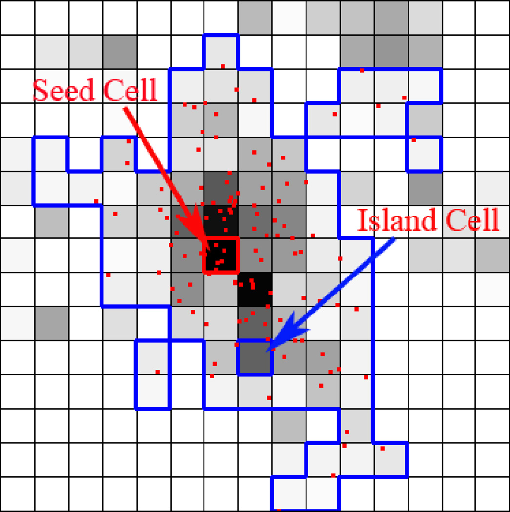
The spatio-temporal clustering process may lead to some island cells that are within but do not belong to a spatio-temporal cluster. For example, if a seed cell cannot form a spatio-temporal cluster but is within the boundary of an existing cluster, then this cell exhibits an ‘island’ within the detected cluster (illustrated in Figure 6). In these cases, the island cells are set to be automatically merged into the containing cluster.
Figure 6.
An example of a spatio-temporal cluster detected by the Queen-based growing method. The cluster area is delineated by blue lines; red points are the GPS points within the cluster; the cell with a red boundary is the cluster center (seed cell); there is also an island cell located near the bottom of the cluster. The island cell would be merged into the existing cluster.
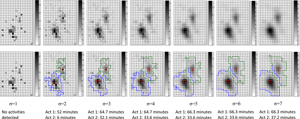
Figure 7 shows the spatio-temporal clusters detected at different smoothing levels. The first smoothed image (shown in the first column of images in the figure, σ=1) did not yield any spatio-temporal clusters. However, two sub-locations (which correspond to the stays at buildings A and C) appeared at the second iteration (σ=2). The size and duration of the two clusters grew gradually with the increase of σ. This pattern of cluster evolution will be captured in the next section.
Figure 7.
Spatio-temporal clusters detected at different levels of smoothing. The upper image for each σ value represents the smoothed cells, and the lower image depicts the extent of the detected spatio-temporal clusters, which are used to represent sub-locations. The cluster depicted by the blue boundary represents the first staying activity in building A shown in Figure 1; the cluster depicted by the green boundary represents the second staying activity in building B. The red cell denotes the cluster center. The duration of each activity is calculated using the k-neighborhood point aggregation method.
Cluster affiliation and sub-location identification
A unique characteristic of scale space representation is that, as smoothing increases, local features gradually merge into larger features, which better denote the overall structure of the image (Leung et al. 2000). As shown in Figure 7, a spatio-temporal cluster identified at a specific σ may be only a part of a larger cluster (which would be identified at a larger σ) and may not be able to represent an entire sub-location. Therefore, we took advantage of the pyramid structure of clusters to derive complete sub-locations of a detected activity. This work was based on two definitions of cluster linkage: temporal link and spatial link. A temporal link was established between two clusters at neighboring layers (i.e., σi and σi+1) if the duration period (i.e., measured from the starting point of the first long segment to the ending point of the last long segment) of the cluster at the lower level, σi, was included in that of the cluster at the higher level, σi+1. A spatial link was established between two clusters at neighboring layers if their seed cells were within the queen neighborhood of each other. Using these two criteria, each cluster identified at a specific σi was assigned an affiliation status that could be No Affiliation, False Affiliation, or True Affiliation. No Affiliation was defined as a situation in which the current cluster, cit, had no temporal link to any clusters at σi+1. False Affiliation was defined as a situation in which cit was temporally linked but not spatially linked to a cluster at σi+1. And True Affiliation was defined as a situation in which cit was both temporally and spatially linkable to the same cluster at σi+1. From the definitions, we can see that clusters with No Affiliation can be interpreted as independent clusters because they cannot be merged into any upper level clusters. A False Affiliation is primarily caused by the smoothing effect of the Gaussian function or random errors instead of the inherent relationship between clusters. However, a True Affiliation represents a self-adaptation of an activity that was not completed derived at a lower level. In other words, a temporal link (resulting in either a False Affiliation or a True Affiliation) identifies pairs of clusters that are potentially linkable. The differentiation between False Affiliation and True Affiliation ensures that the linkage is due to spatio-temporal connectedness instead of to the effect of smoothing. Therefore, at each layer that corresponds to σi, clusters with No Affiliation or False Affiliation were retained and recorded to represent a sub-location of the staying activity. Clusters with True Affiliation remained in the iteration until they became nonaffiliated or falsely affiliated, or until they reached the iteration stop criterion, whichever occurred first. We defined the iteration stop criterion as a situation in which a cluster’s duration period remained unchanged for four consecutive σs.
Next, we used the group of spatio-temporal clusters listed in Figure 7 to illustrate the process of cluster affiliation and sub-location identification. For the first spatio-temporal cluster, c21, (i.e., the one with blue boundary and a duration of 52 minutes) identified at σ=2, we found that its duration was within that of the first cluster, c31, (i.e., the one with blue boundary and a duration of 64.7 minutes) identified at σ=3. Therefore, a temporal link was established between c21 and c31. Since the seed cells of the two clusters were queen neighbors of each other, a spatial link was also established between them. On the basis of the two links, we concluded that c21 was truly affiliated to c31. Similarly, the second cluster, c22, identified at σ=2 was determined to be truly affiliated to c32 at σ=3. No cases of False Affiliation or No Affiliation were found during the process. The affiliation process of the first cluster continued until the σ value reached 8 (the images for σ=8 are not shown in Figure 7 due to space constraints), because at this value the duration value remained stable (i.e., 66.3 minutes) for four consecutive σ values. Therefore, this sub-location was identified and recorded. Similarly, the affiliation process of the second cluster stopped at the σ value of ten (image not shown), with the stable duration of 37.2 minutes. The scale-adaptive clustering method stopped here because all sub-locations of the activity had been determined. The center cells of the sub-locations were then overlayed with GIS layers to obtain information about indoor/outdoor environments and to infer trip purposes. Note that due to systematic errors of GPS location and the influence of indoor-shielding, the detected seed cell may have fallen at or close to the border of the building. To address this problem, we used the three-meter buffer area of the building instead of the real foot print to infer indoor/outdoor environments: if the seed cell fell within the buffer, then the sub-location was determined as indoor. Using this criterion, we determined that both sub-locations identified in Figure 7 were inside the building. The trip purpose of the sub-location could be inferred by the building attribute (e.g., office building, shopping center, gym).
4. Methodology Evaluation
Since the accuracy of the fuzzy classification method has already been evaluated in a previous study (Wan and Lin 2016), the evaluation in this current study will primarily focus on the scale-adaptive method. Specifically, we first assessed the robustness of the scale-adaptive method on model parameters based on GPS points shown in Figure 1. Then, the overall accuracy of the method was evaluated based on historical GPS data sets.
4.1 Robustness evaluation
The robustness evaluation focused on two parameters that may influence the clustering and iteration results: cell size and segment threshold duration. The evaluation was implemented on the staying activity shown in Figure 1 only. For both parameters, we wanted to know how their variations influenced the robustness of the algorithm. Specifically, for the first parameter, we tested a group of cell sizes ranging from one to ten meters, in one meter increments. We evaluated the growing pattern of activity duration with different cell sizes. For the segment threshold duration parameter, we tested eleven values ranging from sixty seconds to 600 seconds, with the increment of sixty seconds. We evaluated the probability of misclassifications with the change of the threshold value.
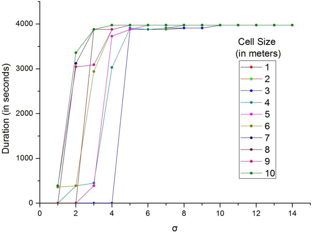
Figure 8 shows the evaluation result based on different cell sizes for the first activity in Figure 1. To be consistent with previous illustrations, the duration threshold value was set to be 300 seconds. In general, iterations based on all cell sizes were able to detect the spatio-temporal cluster, as the iterations all stopped at the duration of 3975 seconds. However, it was also observed that larger cell sizes corresponded to quicker detection of the cluster and faster iteration stopping. For example, the spatio-temporal cluster was first detected at the σ of four for the cell size of 1 meter. For larger cell sizes, such as six, nine, and ten meters, the cluster was already identified at the first σ value. In addition, the iteration stopped at the σ value of twelve for the cell size of one meter, but at the σ value of seven for the cell size of ten meters. It is worth noting that the increased speed was based on the sacrifice of location accuracy, as larger cell sizes generated coarser locations of the activity. A separate evaluation on the second activity revealed a similar pattern to that of the first activity. Therefore, the result of the second activity is not shown here.
Figure 8.
The influence of cell size on spatio-temporal cluster detection by the scale-adaptive method (note: the evaluation was based on the first sub-location in Figure 1; the duration value of 0 means that the activity was not detected at the specific σ value for the specific cell size).
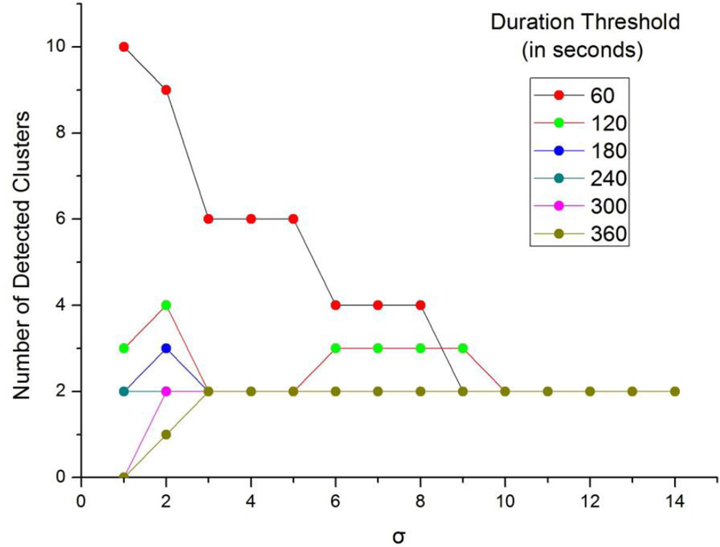
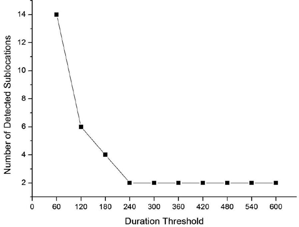
Figures 9 and 10 show how the number of detected spatio-temporal clusters (Figure 9) and the number of detected sub-locations (Figure 10) changed with the duration threshold. Generally, smaller duration thresholds led to more spatio-temporal clusters and sub-locations. For example, the threshold value of sixty seconds yielded ten spatio-temporal clusters at the σ value of one. The cluster iteration at this same threshold value detected fourteen sub-locations, which was many more than the actual number (i.e., two). However, an increased threshold value could help eliminate this type of error. As can be seen from the figures, with the increase of the threshold, the numbers of spatio-temporal clusters and the detected sub-locations both decreased until reaching the threshold of 240 seconds, where both numbers remained at two. Sub-locations detected at thresholds larger than 240 seconds both had the same duration as those shown in Figure 8.
Figure 9.
The influence of duration threshold on spatio-temporal cluster detection and iteration (Note: the evaluation was based on the two sub-locations shown in Figure 1.)
Figure 10.
The influence of duration threshold on sub-location identification (Note: the evaluation was based on the two sub-locations shown in Figure 1.)
4.2 Overall accuracy evaluation
The overall performance of the proposed methodology was evaluated on a set of GPS datasets collected in two previous studies (Wan and Lin 2013; Wan and Lin 2016). These datasets were collected between January 1, 2012, through March 30, 2013, by three free-living subjects using different types of smartphones, including a Nokia N900, a Samsung Galaxy Note I, and a Motorola Droid. These phones were set to automatically record GPS data at a five-second interval when the phone was on. The observation period was fourteen days for the subject who carried the Nokia phone, seventeen days for the subject who carried the Samsung phone, and fifteen days for the subject who carried the Motorola phone. During the observation period, each subject was asked to turn on the phone when they get up and turn it off before doing to bed, to carry the phone with them as much as possible, and to record information of their activities (e.g., start time, end time, trip purpose) in a notebook. A total of 88,833 GPS points were collected during the data collection period. This number is smaller than expected because two subjects’ working places are inside a building where GPS signals were barely received. This leads to extensive data loss when the subjects were working during weekdays. After the GPS data was downloaded to a computer every week, each subject performed a GIS-based recall to correct mistakenly-recorded activities and to recover activities that were not recorded in the notebook but were reflected in the GPS data (Wan and Lin 2013). Subjects were also asked to identify sub-locations of staying activities by overlaying the GPS points with GIS layers and Google Earth. The validation process identified a total of 448 activities that were labeled as either staying, walking, or other transportation based on our definition of activities. Information (e.g., starting time, ending time, trip purpose, sub-locations (if any)) on these activities will be used as the reference for result evaluation. These activities are referred to as ‘baseline activities’ in subsequent parts of this article. The data collection and analysis were reviewed and approved by the IRB of the University of Nebraska Medical Center.
Before the fuzzy classification, the original five-second dataset was re-sampled at fifteen-seconds because point characteristics such as speed and angle are believed to be more reliable at this interval (Wan and Lin 2013; Wan and Lin 2016). All GPS data underwent a pre-processing procedure to remove any blatantly incorrect points and to overcome data loss caused by GPS cold start or indoor shielding (Wan and Lin 2013). The fuzzy classification method was then implemented on the entire dataset to differentiate activity patterns. Next, the scale-adaptive algorithm was applied on all staying activities to identify sub-locations. On the basis of the results of robustness evaluation in last section, we set the raster cell size to be seven meters and the duration threshold to be 300 seconds.
The fuzzy classification method estimated 474 activities, among which 422 matched with a specific baseline activity and 20 did not match any baseline activities. Among the correctly identified activities, 210 were staying activities and the rest are staying and other transportation activities. 32 of the staying activities were ascertained by the subjects as having more than one sub-locations. Since the major purpose of the scale-adaptive method is to determine sub-locations of staying activities, our evaluation will focus on these 210 activities only. For walking and other transportation activities, map matching methods could be used to determine routes and street names of the routes (Ghys et al. 2009).
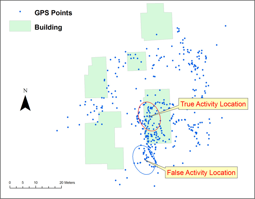
The scale-adaptive method determined that 34 out of the 210 correctly identified staying activities had sub-locations, of which 31 matched with the subject-recorded reference data and three corresponded to false detection (i.e., an activity was recorded by the subject as having a single location but was detected by the algorithm as a multi-location activity). We found that the major reason for these false detections was the very high level of location deviation of the GPS points (shown in Figure 11 where a subject stayed in a house with dense trees around for 17 hours). All three false detections were indoor-staying activities, for which signal shielding is a substantial concern. The long duration of these activities led to a high number of GPS points, which also increased the likelihood that several consecutive points would cluster together to form a false sub-location.
Figure 11.
An example of false detection by the scale-adaptive clustering method. The GPS points reflect an indoor staying activity (duration is approximately seventeen hours) inside the building on the lower right corner. However, the algorithm identified two sub-locations: one corresponds to the true activity location (shown inside the red circle) and the other points to a location (shown in the blue circle) that the subject had not been to during the observation period. The false activity location were observed when the subject was staying in the basement where there was substantial GPS signal shielding.
In addition, the algorithm identified a multi-location activity as a single-location activity. An examination of this activity’s point structure found that the misidentification was due to the duration threshold, as one sub-location had a duration of only 161 seconds, much shorter than the 300-seconds duration threshold used in the algorithm.
5. Discussion and Conclusion
Portable GPS units are becoming increasingly popular as a means of measuring human activities in environment-health studies. However, uncertainties that come with location inaccuracy and data inconsistency have impeded the effective use of these units. To address these challenges, this article presented an integrated approach for deriving meaningful activity information from individual-collected GPS data. Specifically, a fuzzy classification method was first adopted to derive coarse activity categories. Then, a scale-adaptive method was developed to infer detailed information about staying activities. This scheme was designed to overcome different types of uncertainties at different stages of GPS data processing. Evaluation based on smartphone-collected GPS data revealed desirable performance of this scheme.
The methodological framework described in this study contributes to both theoretical and applied aspects of geography and public health. For example, the basic idea of the scale-adaptive method stems from the theories of spatial clustering and scale-space. On the basis of these two theories, we further extended their applicability to deal with GPS point data and to incorporate temporal continuity beyond spatial proximity. In addition, by introducing a new way to infer correct activity location from incorrect point data, the two methods provide new insights into location uncertainty analyses. To the best of our knowledge, this is among the first studies to assess location uncertainties of smartphone GPS points and the first to develop a complete methodological framework to address the uncertainties. From the application perspective, the GPS data processing framework will benefit investigations into functional status, physical activity promotion, and environmental exposure. The methods are also adaptable to location data collected by sources such as the Global Navigation Satellites System (GNSS) and even indoor location sensors (e.g., Wi-Fi, RFID), which work similarly to GPS satellites.
This study used a series of historical GPS data to evaluate the two methods. A potential limitation of these datasets is that they were collected by a limited number of subjects (n= 3), which may not be representative of a large population. However, the data cover almost all types of human activities (e.g., walking, shopping, dinning, and driving) under various shielding conditions (e.g., open area, under trees, urban canyon, and inside buildings) which represent a wide range of location uncertainties to the GPS points. The high compliance of the subjects in data collection and journal recording also provides good quality data of GPS points and baseline activities, which greatly facilitated the evaluation procedure.
Some future work is needed to perfect the approach proposed in this article. First, the flexibility of the algorithm parameters should be enhanced. For example, this study evaluated the influence of the two primary parameters (i.e., cell size and duration threshold) of the scale-adaptive method. We found that larger cell sizes led to faster detection of spatio-temporal clusters but lower spatial resolution of the sub-locations. This limitation could be solved by using flexible cell sizes. For example, large cell sizes could be used at small σ values to determine the existence of spatio-temporal clusters. Then, small cell sizes could be applied on the cluster area to refine sub-locations. By using flexible cell sizes, both the iteration speed and the spatial resolution could be guaranteed.
Second, the algorithms should be enhanced to handle more complex activity patterns. The activity used for illustration in this article and those used in the comprehensive evaluation were based primarily on two sub-locations. When there are multiple and back-and-forth sub-locations within an activity (for example, when the sequence of sub-locations is “home->yard->home->yard”), the scale-adaptive method may not be effective. In such a case, it is necessary to incorporate a duration checking procedure into the cluster iteration process to identify the complex patterns.
Third, multiple data sources could be used to overcome the misclassification problem. For example, the accelerometer function of smartphones could be used to complement the GPS function, because the acceleration information provides another dimension of human activities (Schenk et al. 2011). Accelerometer data could help researchers to classify the ‘staying’ activities into more detailed categories such as indoor walking and sitting. In the case of the misclassification in Figure 11, the false activity location may have been distinguishable if the measured acceleration pattern showed little change during the entire observation period. Although integrating multi-source data to improve activity inference represents the future, a robust GPS data classification framework is the very basic step towards this goal, because GPS-derived activities provides unique information about the spatial context of various activities.
In conclusion, this article describes a methodological framework for deriving continuous activity information from individual collected GPS data while overcoming location uncertainties of the data. This framework showed satisfactory accuracy on revealing individual’s activities and indoor/outdoor environments and showed great potential in environmental health studies.
Acknowledgments
Research reported in this publication was supported by the National Institute On Aging of the National Institutes of Health under Award Number R03AG044759. The content is solely the responsibility of the authors and does not necessarily represent the official views of the National Institutes of Health.
Footnotes
Conflicts of interest: The authors identify no conflicts of interest in this work.
References
- Ankerst M, Breunig MM, Kriegel H, Sander J. Proceedings of the ACM SIGMOD’99 International Conference on Management of Data. Philadelphia PA: 1999. OPTICS: Ordering Points To Identify the Clustering Structure. 1999. [Google Scholar]
- Ashbrook D, Starner T. Using GPS to learn significant locations and predict movement across multiple users. Pers Ubiquitous Comput. 2003;7:275–286. [Google Scholar]
- Babaud J, Witkin AP, Baudin M, Duda R. Uniquenes of the Gaussian kernel for scale-space filtering. IEEE Trans Pattern Analysis and Machine Intell. 1986;8(1):26–33. doi: 10.1109/tpami.1986.4767749. [DOI] [PubMed] [Google Scholar]
- Bowling A. Mode of questionnaire administration can have serious effects on data quality. Journal of Public Health. 2005;27:281–291. doi: 10.1093/pubmed/fdi031. [DOI] [PubMed] [Google Scholar]
- Carlson RH, Huebner DR, Hoarty CA, Whittington J, Haynatzki G, Balas MC, Schenk AN, Goulding EH, Potter JF, Bonasera SJ. Treadmill gait speeds correlate with physical activity counts measured by cell phone accelerometers. Gait Posture. 2011;36(2):241–248. doi: 10.1016/j.gaitpost.2012.02.025. [DOI] [PMC free article] [PubMed] [Google Scholar]
- Chen C, Bian L, Ma J. From traces to trajectories: How well can we guess activity locations from mobile phone traces? Transportation Research Part C. Emerging Technologies. 2014;46:326–337. [Google Scholar]
- Ciucu M, Heas P, Mihai D, Tilton J. Scale space exploration for mining image information content. In: Zaiane OR, Simoff SJ, Djeraba C, editors. Mining Multimedia and Complex Data. 2003. pp. 118–133. [Google Scholar]
- Cooper AR, Page AS, Wheeler B, Griew P, Davis L, Hillsdon H, Jago R. Mapping the walk to school using accelerometry combined with a Global Positioning System. American Journal of Preventive Medicine. 2010;38(2):178–183. doi: 10.1016/j.amepre.2009.10.036. [DOI] [PubMed] [Google Scholar]
- Duan L, Xu L, Guo F, Lee J, Yan B. A local-density based spatial clustering algorithm with noise. Information Systems. 2007;32:978–986. [Google Scholar]
- Elgethun K, Yost MG, Fitzpatrick CT, Nyerges TL, Fenske RA. Comparison of global positioning system (GPS) tracking and parent-report diaries to characterize children’s time-location patterns. Journal of exposure science & environmental epidemiology. 2007;17:196–206. doi: 10.1038/sj.jes.7500496. [DOI] [PubMed] [Google Scholar]
- Ester M, Kriegel H, Sander J, Xu X. Proceedings of 2nd International Conference on Knowledge Discovery and Data Mining. Menlo Park, California: AAAI Press; 1996. A Density-Based Algorithm for Discovering Clusters in Large Spatial Databases with Noise; pp. 226–231. [Google Scholar]
- Ghys K, Kuijpers B, Moelans B, et al. Map matching and uncertainty: an algorithm and real-world experiments; Proceedings of the 17th ACM SIGSPATIAL International Conference on Advances in Geographic Information Systems; 2009. pp. 468–471. [Google Scholar]
- Guc B, May M, Saygin Y, Körner C. Proceedings of the 11th AGILE International Conference on Geographic Information Science. Girona, Spain: 2008. Semantic annotation of GPS trajectories. [Google Scholar]
- Herrmann SD, Snook EM, Kang M, Scott CB, Mack MG, Dompier TP, Ragan BG. Development and validation of a movement and activity in physical space score as a functional outcome measure. Archives of physical medicine and rehabilitation. 2011;192:1652–1658. doi: 10.1016/j.apmr.2011.05.001. [DOI] [PubMed] [Google Scholar]
- Hirsch JA, Winters M, Clarke P, McKay H. Generating GPS activity spaces that shed light upon the mobility habits of older adults: a descriptive analysis. International journal of health geographics. 2014;13(1):51. doi: 10.1186/1476-072X-13-51. [DOI] [PMC free article] [PubMed] [Google Scholar]
- Jankowska M, Schipperijn J, Kerr J. A Framework for Using GPS Data in Physical Activity and Sedentary Behavior Studies. Exercise and sport sciences reviews. 2015;43(1):48–56. doi: 10.1249/JES.0000000000000035. [DOI] [PMC free article] [PubMed] [Google Scholar]
- Kaufman L, Rousseeuw PJ. Finding Groups in Data: An Introduction to Cluster Analysis. Wiley; 1990. [Google Scholar]
- Koenderink JJ. The structure of images. Biological Cybernetics. 1984;50:363–370. doi: 10.1007/BF00336961. [DOI] [PubMed] [Google Scholar]
- Kwan MP. Analysis of human spatial behavior in a GIS environment: recent developments and future prospect. Journal of Geographical Systems. 2000;2(1):85–90. [Google Scholar]
- Leung Y, Zhang JS, Xu ZB. Clustering by scale space filtering. IEEE Transactions on Pattern Analysis and Machine Intelligence. 2000;22:1396–1410. [Google Scholar]
- Liao L, Fox D, Kautz H. Extracting places and activities from GPS traces using hierarchical conditional random fields. The International Journal of Robotics Research. 2007;26:119–134. [Google Scholar]
- Lindeberg T. Scale-space for discrete signals. IEEE Transactions on Pattern Analysis and Machine Intelligence. 1990;12(3):234–254. [Google Scholar]
- Lindeberg T. Scale-space theory in computer vision. Boston: Kluwer Academic; 1993. [Google Scholar]
- Lindeberg T. Feature detection with automatic scale selection. Int J Comput Vis. 1998;30(2):77–116. [Google Scholar]
- Luo J, Zhou C, Leung Y, Zhang Y, Huang Y. Scale-space theory based regionalization for spatial cells. ACTA Geographica Sinica. 2002;57(2):167–173. [Google Scholar]
- Mamdani EH, Assilian S. An experiment in linguistic synthesis with a fuzzy logic controller. International journal of man-machine studies. 1975;7(1):1–13. [Google Scholar]
- Montoliu R, Gatica-Perez D. Proceedings of 9th International Conference on Mobile and Ubiquitous Multimedia. MUM; 2010. Discovering human places of interest from multimodal mobile phone data. [Google Scholar]
- Mu L, Wang F. A scale-space clustering method: mitigating the effect of scale in the analysis of zone-based data. Ann Assoc Am Geogr. 2008;98:85–101. [Google Scholar]
- Ng R, Han J. Proceedings of the International Conference on Very Large Data Bases. Santiago, Chile: 1994. Efficient and Effective Clustering Method for Spatial Data Mining; pp. 144–155. [Google Scholar]
- Richardson DB, Volkow ND, Kwan MP, Kaplan RM, Goodchild MF, Croyle RT. Spatial turn in health research. Science. 2013;339(6126):1390–1392. doi: 10.1126/science.1232257. [DOI] [PMC free article] [PubMed] [Google Scholar]
- Schenk AK, Witbrodt BC, Hoarty CA, Carlson RH, Goulding EH, Potter JF, Bonasera SJ. Cellular telephones measure activity and life-space in community-dwelling adults: proof of principle. Journal of the American Geriatric Society. 2011;59:345–352. doi: 10.1111/j.1532-5415.2010.03267.x. [DOI] [PMC free article] [PubMed] [Google Scholar]
- Schüssler N, Axhausen KW. Paper presented at the 88th Annual Meeting of the Transportation Research Board. Washington, DC: 2009. Processing GPS raw data without additional information. [Google Scholar]
- Steinle S, Reis S, Sabel C, Semple S, Twigg M, et al. Personal exposure monitoring of PM 2.5 in indoor and outdoor microenvironments. Science of the Total Environment. 2015;508:383–394. doi: 10.1016/j.scitotenv.2014.12.003. [DOI] [PubMed] [Google Scholar]
- Takagi K, Sugeno M. Fuzzy identification of systems and its applications to modeling and control. IEEE Transactions on Systems, Man and Cybernetics. 1985;15:116–132. [Google Scholar]
- Thierry B, Chaix B, Kestens Y. Detecting activity locations from raw GPS data: a novel kernel-based algorithm. International journal of health geographics. 2013;12:14. doi: 10.1186/1476-072X-12-14. [DOI] [PMC free article] [PubMed] [Google Scholar]
- Tung JY, Semple JFL, Woo WX, Hsu WS, Sinn M, Roy EA, Poupart P. Proceedings of the 2011 Annual Conference of the Rehabilitation Engineering and Assistive Technology Society of North America (RESNA) Toronto, Canada: 2011. VALMA: voice, activity and location monitoring for Alzheimer's disease and related dementias. [Google Scholar]
- Wan N, Lin G. Life-space characterization from cellular telephone collected GPS data. Computers, Environment and Urban Systems. 2013;39:63–70. [Google Scholar]
- Wan N, Lin G. Classifying Human Activity Patterns from Smartphone Collected GPS data: a Fuzzy Classification and Aggregation Approach. Transactions in GIS. 2016 doi: 10.1111/tgis.12181. [DOI] [PMC free article] [PubMed] [Google Scholar]
- Wan N, Qu W, Whitington J, Witbrodt B, Henderson M, Goulding E, Schenk A, Bonasera S, Lin G. Assessing smart phones for generating life space indicators. Environmental and Planning B. Planning and Design. 2013;40(2):350–361. doi: 10.1068/b38200. [DOI] [PMC free article] [PubMed] [Google Scholar]
- Wheeler B, Cooper A, Page A, Jago R. Greenspace and children’s physical activity: a GPS/GIS analysis of the PEACH project. Preventive medicine. 2010;51:148–152. doi: 10.1016/j.ypmed.2010.06.001. [DOI] [PubMed] [Google Scholar]
- Whyatt D, Pooley C, Coulton P, Moser M, Bamford W, Davies G. Estimating personal exposure to air pollution on the journey to and from school using GPS, GIS, and mobile phone technology; Proceedings of the 11th International Conference on Harmonisation within Atmpspheric Dispersion Modeling for Regulatory Purposes; 2007. [Google Scholar]
- Wiehe SE, Carroll AE, Liu GC, Haberkorn KL, Hoch SC, Wilson JS, Fortenberry JD. Using GPS-enabled cell phones to track the travel patterns of adolescents. International journal of health geographics. 2008;7:22. doi: 10.1186/1476-072X-7-22. [DOI] [PMC free article] [PubMed] [Google Scholar]
- Witkin AP. Proc. 8th Int Joint Conf Art Intell. Karlsruhe, West Germany: 1983. Scale-space filtering; pp. 1019–1022. [Google Scholar]
- Wong YF, Posner EC. A new clustering algorithm applicable to multispectral and polarimetric SAR images. IEEE Trans Geosci RemoteSens. 1993;31(3):634–644. [Google Scholar]
- Wu J, Jiang C, Houston D, Baker D, Delfino R. Automated time activity classification based on global positioning system (GPS) tracking data. Environmental Health. 2011;10:101. doi: 10.1186/1476-069X-10-101. [DOI] [PMC free article] [PubMed] [Google Scholar]
- Yuille AL, Poggio TA. Scale theorems for zero crossings. IEEE Transactions on Pattern Analysis and Machine Intelligence. 1986;8(1):15–25. doi: 10.1109/tpami.1986.4767748. [DOI] [PubMed] [Google Scholar]
- Zhang L, Dalyot S, Eggert D, Sester M. Multi-stage approach to travel-mode segmentation and classification analysis of GPS traces. ISPRS Workshop on Geospatial Data Infrastructure: from data acquisition and updating to smarter services. 2011:87–93. [Google Scholar]
- Zheng Y, Liu L, Wang L, Xie X. Paper presented at the 17th World Wide Web conference. Beijing, China: 2008. Learning transportation mode from raw GPS data for geographic applications on the web. (available at http://research.microsoft.com/pubs/78567/fp485-Zheng.pdf) [Google Scholar]


