Analysis of remotely sensed and surface data of aerosols and meteorology for the Mexico Megalopolis Area between 2003 and 2015

Abstract

This paper presents an aerosol characterization study from 2003 to 2015 for the Mexico City Metropolitan Area using remotely sensed aerosol data, ground-based measurements, air mass trajectory modeling, aerosol chemical composition modeling, and reanalysis data for the broader Megalopolis of Central Mexico region. The most extensive biomass burning emissions occur between March and May concurrent with the highest aerosol optical depth, ultraviolet aerosol index, and surface particulate matter (PM) mass concentration values. A notable enhancement in coarse PM levels is observed during vehicular rush hour periods on weekdays versus weekends owing to nonengine-related emissions such as resuspended dust. Among wet deposition species measured, PM_2.5, PM₁₀, and PM_coarse (PM₁₀−PM_2.5) were best correlated with NH₄⁺, SO₄²⁻, and Ca²⁺, suggesting that the latter three constituents are important components of the aerosol seeding raindrops that eventually deposit to the surface in the study region. Reductions in surface PM mass concentrations were observed in 2014–2015 owing to reduced regional biomass burning as compared to 2003–2013.

1. Introduction

With increasing urbanization, it is expected that 66% of the global population will live in urban conglomerations by 2050 [United Nations, 2015]. This motivates improved understanding of air quality in megacities around the world. In Mexico, two such megacities are the Mexico City Metropolitan Area (MCMA; 2240 m above sea level (asl)), which has over 21 million inhabitants, and the larger Mexico “Megalopolis” Area, known as Megalopolis of Central Mexico, which includes metropolitan zones in the center of Mexico, containing MCMA (Mexico City and municipalities in Mexico State and Hidalgo) and surrounding metropolitan areas (Tulancingo, Pachuca, Tula, Tlaxcala Puebla, Cuautla, Cuernavaca, and Toluca), collectively accounting for over 30 million people (http://www.inegi.org.mx/). Knowledge of the abundance and physicochemical properties of air pollutants, especially particulate matter (PM), is needed to quantify the nature of their interactions with solar radiation and water vapor in the Megalopolis, in addition to their effects on public health. Furthermore, aerosol particles serve as cloud condensation nuclei and ice nuclei, and thus the chemical signature of precipitation is expected to reflect chemical properties of PM in this region.

Parts of the Mexico Megalopolis have been the subject of field measurement studies, modeling activities, and remote sensing studies [Livingston et al., 2009; Redemann et al., 2009; Kar et al., 2015]. For example, the Megacity Initiative: Local and Global Research Observations campaign in 2006 was an international collaborative effort to study the properties, evolution, and transport of atmospheric emissions generated in MCMA [Molina et al., 2010]. The region has diverse pollutant sources including biogenic emissions, biomass burning, extensive anthropogenic activity, and the Popocatepetl volcano in the southeastern part of Mexico City [Molina et al., 2010; Almanza et al., 2012]. Surface measurements of aerosol composition in MCMA suggest that about half of PM₁₀ and PM_2.5 is composed of carbonaceous components, with the remaining half split relatively evenly between dust and secondary inorganic species [Querol et al., 2008; de Foy et al., 2011]. The organic fraction was found to include about half secondary organic aerosol (SOA), with the rest divided between primary urban emissions and biomass burning emissions [Aiken et al., 2009, 2010]. Modeling has indicated that about half of the urban organic carbon in particles stems from motor vehicle emissions [Stone et al., 2008]. Furthermore, microscopy analysis has shown that most particles in MCMA are either coated or comprise aggregates [Adachi and Buseck, 2008].

Terrain and seasonal factors influence air quality in the Megalopolis. Similar to other major urban centers such as Los Angeles [Ryerson et al., 2013] and Tehran [Crosbie et al., 2014] where terrain negatively impacts air quality, mountains on three sides of the MCMA basin trap pollutants, especially during the early morning hours and in winter [de Foy et al., 2006, 2009, 2011; Molina et al., 2007, 2010]. Anthropogenic pollution reaches its maximum influence during the winter due to the shallower mixing layer [Molina et al., 2007]. Biomass burning on the other hand peaks in the spring due to burning in surrounding areas [Bravo et al., 2002; Yokelson et al., 2007].

The goal of this study is to expand upon these previous studies focused on the MCMA region by conducting an updated aerosol characterization study from 2003 to 2015 using remotely sensed aerosol data, surface monitoring data, air mass trajectory modeling, and chemical transport modeling for the broader Megalopolis Area. While the studies noted above have examined aerosol characteristics, a new addition of this study is analysis of how PM is related to precipitation chemistry in the region. This is of interest as it represents a nontraditional way of examining aerosol-cloud precipitations, and knowledge of precipitation chemistry itself has implications for effects on ecosystems after wet deposition. The subsequent analysis is aimed at addressing the following questions: (i) what are the monthly profiles of parameters related to PM in relation to meteorology? (ii) What are the diurnal and weekly profiles of surface aerosol data? (iii) What is the relationship between PM and wet deposition species concentrations? And (iv) how have pollutant concentrations changed from 2003 to 2015?

2. Data and Methods

A diverse set of data is used in this work collected between 2003 and 2015 from sources including ground-based monitoring stations, models, and remote sensors. The central region of Mexico is divided in two nested spatial domains (Figure 1a). Domain 1 (−95° to −106°W, 15° to 22°N; Figure 1b) is the spatial area over which remotely sensed fire and vegetative cover data are examined. Domain 2 (−97 to −100°W, 18 to 20°N; Figure 1c) includes the Central Megalopolis of Mexico where surface monitoring station data and the remaining satellite data were obtained. The data sets are summarized below.

Figure 1.

(a) Mexico divided in two nested spatial domains (red and black squares). The blue lines represent political divisions of the six states of the Central Megalopolis of Mexico. (b) The larger Domain 1 (red box: −95° to −106°W, 15° to 22°N) is examined for fire activity (e.g., red points in June 2011). (c) Amplification of the smaller Domain 2 (black box: −97° to −100°W, 18° to 20°N) is shown, where the salmon-colored areas correspond to populated urban centers and the markers represent surface monitoring stations in the Central Megalopolis: SIMAT-Mexico City (orange pentagons), SEMA-Puebla (blue squares), and SEMA-Toluca (light blue circles). In Figure 1c, the black airplane symbols represent airports and the red diamond marker shows the location of the Mexico City AERONET site.

2.1. Satellite Remote Sensing Data

Remotely sensed data for aerosol particles and other environmental parameters were downloaded from the Goddard Earth Sciences Data and Information Services Center via the GIOVANNI v4.19 portal (http://disc.sci.gsfc.nasa.gov/giovanni). A summary of parameters, instrument data sources, and spatiotemporal resolutions is in Table 1. It is emphasized that the focus with the remote sensing data is not absolute values but rather qualitative monthly trends. Daily aerosol optical depth (AOD) data were used from Moderate Resolution Imaging Spectroradiometer (MODIS-Aqua) Collection 6 [Levy et al., 2013] to represent aerosol abundance in the study region. AOD data were specifically used from the Deep Blue algorithm, which corrects for problems associated with bright land surfaces, including those characterized by a combination of vegetative, arid, and/or urban influence [Hsu et al., 2004, 2013]. As a measure of particle size distribution, Deep Blue Ångström Exponent (AE) data were used from MODIS Aqua/Terra. Since the temporal trends of Aqua and Terra agreed, data are only reported from Aqua. AOD data are also used from the Multiangle Imaging Spectroradiometer (MISR) [Diner and Hansen, 2012]. Data representative of the abundance of light-absorbing aerosols (e.g., dust and smoke) was obtained from the Ozone Monitoring Instrument (Aura/OMI) [Torres et al., 2007] in the form of the ultraviolet aerosol index (UV AI) parameter. There are several important factors that determine the quality assurance of remote sensing data [Kahn et al., 2010; Li et al., 2009]. Among these factors are clouds, which introduce bias in retrievals of aerosol parameters [Ostby et al., 2014; Shi et al., 2014]. To address this issue, we filtered remote sensing data when MODIS-Aqua cloud fraction exceeded 70%.

Table 1.

Summary of Satellite Data Set Details Used for This Study in Domain 2 of Figure 1 (−97° to −100°W, 18° to 20°N)^a

Variable	Short Name	Source	Temporal Resolution	Spatial Resolution	Temporal Range
AOD (550 nm)b	MYD08_D3_v6	MODIS-Aqua	D	1 × 1°	2003–2015
AOD (555 nm)	MIL3DAE v4	MISR	D	0.5 × 0.5°	2003–2015
AE (412–470 nm)b	MYD08_D3_v06	MODIS-Aqua	D	1 × 1°	2003–2015
UV aerosol index	OMTO3d_003	OMI	D	1 × 1°	2004–2015
Cloud fraction	MYD08_M3_v6	MODIS-Aqua	D	1 × 1°	2003–2015
PBLH (m)	M2TMNXFLX	MERRA	M	0.5 × 0.625°	2003–2015
Speciated AOD (550 nm)	g5e520m0c	GOCART v5	M	1 × 1.25°	1998–2009
NDVIc	MOD13C2v5	MODIS-Terra	M	5600 m	2003–2015
BT (K)c	MCD14DL	FIRMS (MODIS-Terra and Aqua)	M	1 km pixel	2003–2015

^aM = monthly, D = daily.

^bDeep blue for land-only.

^cConsiders Domain 1: broader spatial domain of −95° to −106°W, 15° to 22°N.

Intensity, frequency and location of fires between 2003 and 2015 were obtained from the MODIS Collection 6 combined Terra/Aqua (MCD14DL) from the Fire Information for Resource Management System (FIRMS; https://earthdata.nasa.gov/active-fire-data). MODIS Terra overpasses the study region around 04:30 to 05:30 Greenwich mean time (GMT; ascend) and 17:00 to 18:00 GMT (descend), while MODIS Aqua passes over between 07:30 to 08:30 GMT (descend) and 19:30 to 20:30 GMT (ascend). The method relies on detection of thermal anomalies, specifically with the brightness temperature (BT) parameter, for quantification of fire intensity [Giglio et al., 2016].

As a proxy for the influence of biogenic volatile organic compound emissions on aerosol characteristics in the study region, data from the normalized difference vegetation index (NDVI) product were used from the MODIS Terra sensor [Bhandari and Kumar, 2012].

The ensuing discussion of results includes comparisons of data with different spatial resolutions, notably between satellite data and surface measurements of aerosol particles. The comparisons of different data sets hinge on monthly mean values, which have been shown to improve the correlation between satellite and surface data [Li et al., 2013, 2014a, 2014b]. We assume in the discussion of comparisons of data sets that those measurements obtained over monthly time scales at the surface are intercomparable with the wider area around the measurement sites in the study region. This has also been done in earlier work in regions such as the United States [Li et al., 2015; Lopez et al., 2016].

2.2. Ground-Based Measurements

Figure 1c shows the area corresponding to the Mexico Central Megalopolis. Within this domain, Mexico City is located in a flat basin that is open and adjoined with Hidalgo, to the north. The remaining three sides are surrounded by high mountains that separate Mexico City from other important urban centers including Puebla (to the southeast), Toluca (west), Morelos (south), and Tlaxcala (east). Ground-based measurements were obtained from sites across the Megalopolis that had at least 70% data coverage on a yearly basis for the 2003 to 2015 period. The resulting sites include five in Mexico City affiliated with the Automatic System of Atmospheric Monitoring (SIMAT; http://www.aire.df.gob.mx), six in Toluca (SEMA-ZMVT), and five in Puebla (SEMA-Puebla). Table 2 summarizes the meteorological parameters and particulate matter (PM₁₀, and PM_2.5) measured at each station, which are briefly introduced below.

Table 2.

Summary of Surface Monitoring Station Details

SIMAT (Mexico) PM2.5, PM10, Wind Speed, Wind Direction, T, RH, Wet Deposition
Station Name	Alias	Latitude (°N)	Longitude (°W)	Time Range	Missing Dataa
Merced	MER	19.425	−99.120	2003–2015	32.4/20.2
Pedregal	PED	19.325	−99.204	2003–2015	24.4/22.4
San Agustin	SAG	19.533	−99.030	2003–2015	34.5/22.3
Tlalpan	TLA	19.529	−99.205	2003–2015	33.4/22.7
Xalostoc	XAL	19.526	−99.082	2003–2015	82.3/22.2
Puebla-SEMA PM10, Wind Speed, Wind Direction, T, RH
Station Name	Alias	Latitude (°N)	Longitude (°W)	Time Range	Missing Dataa
Tecnologico	TEC	19.057	−98.151	2003–2009	−/58.9
Normal	SER	19.067	−98.224	2003–2009	−/67.6
Ninfas	NIN	19.041	−98.214	2003–2007; 2011–2014	−/55.4
Agua Santa	AGS	18.987	−98.250	2003–2008; 2010–2014	−/33.6
Velodromo	VEL	18.987	−98.278	2012–2014	−/84.21
Toluca-SEMA PM10, Wind Speed, Wind Direction, T, RH
Station Name	Alias	Latitude (°N)	Longitude (°W)	Time Range	Missing Dataa
Centro	CE	19.278	−99.656	2003–2008; 2011–2014	−/27.5
Oxtotitlan	OX	19.283	−99.683	2003–2014	−/17.3
Aeropuerto	AP	19.334	−99.574	2003–2015	−/57.9
San Cristobal	SC	19.327	−99.634	2003–2007; 2009–2014	−/19.6
Metepec	MT	19.270	−99.595	2003–2006; 2008–2014	−/30.0
Atenco	SM	19.280	−99.542	2003–2015	−/28.0
SENEAM RH, Precipitation
Station Name	Alias	Latitude (°N)	Longitude (°W)	Time Range	Missing Dataa
Mexico Int Airport	S-Mex	19.435	−99.069	2003–2015	NA
Toluca Int Airport	S-Tol	19.337	−99.566	2003–2015	NA
Puebla Airport	S-Pue	19.158	−98.371	2003–2015	NA
AERONET
AOD, Water Vapor
Station Name	Alias	Latitude (°N)	Longitude (°W)	Time Period	Missing Dataa
Mexico City	N/A	19.334	−99.182	2003–2015	NA

^aPercentage of missing PM_2.5 and PM₁₀ data with respect to the entire 2003–2015 period (PM_2.5/PM₁₀).

2.2.1. Particulate Matter

Particulate matter (PM₁₀ and PM_2.5) data from 2003 to 2015 were obtained from the SIMAT network in the following five zones of Mexico City: Merced (MER) in the central area, Pedregal (PED) to the southeast, San Agustin (SAG) to the northwest, Tlalpan (TLA) to the north, and Xalostoc (XAL) to the northwest. For the various sites in Puebla-SEMA and Toluca-SEMA listed in Table 2, only PM₁₀ was measured. As shown in Table 2, data availability was generally higher for PM₁₀ as compared to that for PM_2.5. Continuous particulate monitors, Beta Attenuation Particle Monitor 1020, or R&P Model 1400a tapered element oscillating microbalances were used to measure PM₁₀, while the Thermo Model 1405-DF Filter Dynamics Measurement Systems method was used to measure both PM₁₀ and PM_2.5 at hourly time resolution. PM_coarse is also discussed in this work and refers to the following difference: PM₁₀−PM_2.5.

2.2.2. Meteorology

Ambient temperature, wind speed, wind direction, and relative humidity (RH) data were collected from Mexico City (SIMAT), Puebla-SEMA, and Toluca-SEMA monitoring networks. Wet deposition chemistry data were also obtained from the SIMAT monitoring network at weekly time resolution, with speciation including major water-soluble cations (Ca²⁺, K⁺, Mg²⁺, Na⁺, and NH₄⁺) and anions (Cl⁻, NO₃⁻, and SO₄²⁻). Precipitation data were obtained from the Navigation Services of Mexican Airspace (SENEAM) at airports in Toluca (−99.57°W, 19.34°N), Mexico City (−99.07°W, 19.4°N), and Puebla (−98.37°W, 19.16°N).

2.2.3. AERONET

Aerosol optical depth (AOD) and columnar water vapor data were obtained from the Aerosol Robotic Network (AERONET, Level 2.0; http://aeronet.gsfc.nasa.gov/) [Holben et al., 1998; Kahn et al., 2005; Perez-Ramirez et al., 2014] for the period between 2003 and 2015 to compare with monthly patterns of corresponding satellite remote sensing data. The AERONET monitoring site used for this study is located in the southwestern part of Mexico City (−99.18°W, 19.33°N; 2268 m asl).

2.3. Air Mass Transport Modeling

To examine air mass source origins impacting the study region, 4 day back trajectories were produced using the Hybrid Single-Particle Lagrangian Integrated Trajectory (HYSPLIT) model [Stein et al., 2015; Rolph, 2016]. The model was run using the National Center for Atmospheric Research and the National Centers for Environmental Prediction reanalysis data with the isentropic vertical velocity method. Data were collected for air masses ending 500 m above the Merced SIMAT station located in central MCMA (19.42°N, 99.12°W; 2245 m asl) between 2003 and 2015. A clustering algorithm [Jorba et al., 2004; Toledano et al., 2009] was used to construct quarterly (December–February, DJF; March–May, MAM; June–August, JJA; September–November, SON) trajectory frequency maps, which present the most frequent transport pathways of air ending in the study region. We note that while the study region is in a high-altitude tropical location with three seasons, as will be discussed further below, annual quarters will be used for discussion of air trajectories to obtain finer temporal resolution as has been done by others for the region [Carreon-Sierra et al., 2015].

2.4. Goddard Ozone Chemistry Aerosol Radiation and Transport (GOCART) Model

In order to examine the column-integrated abundance of major aerosol constituents in the study region, GOCART v5 model data for AOD were used for numerous species including dust, sea salt, sulfate, black carbon (BC), and organic carbon (OC) [Chin et al., 2014]. Data at 1° × 1.25° resolution were examined from 1998 until 2009, the last year of which such data could be obtained. The model uses assimilated meteorological data from the Goddard Earth Observing System Data Assimilation System to generate an analysis of the initial state in order to improve agreement between numerical model and available data. The model includes sulfur, dust, OC and BC, and sea salt emissions [Olivier et al., 1996; Andres and Kasgnoc, 1998; Cook et al., 1999; Duncan et al., 2003], in addition to transport, chemistry, removal via dry and wet deposition [Wesely, 1989; Lin and Rood, 1996; Helfand and Labraga, 1988], and consideration of aerosol optical thickness [Chin et al., 2002].

2.5. Modern Era-Retrospective Analysis for Research and Applications Reanalysis Data

The Modern Era-Retrospective Analysis for Research and Applications (MERRA-2) model [Rienecker et al., 2008] was used to obtain data for planetary boundary layer height (PBLH; M2TMNXFLX_V5.12.4) at 0.5° × 0.625° spatial resolution, over the region in Domain 2 (black box: −97° to −100°W, 18° to 20°N) shown in Figure 1c.

3. Results

3.1. Meteorological Context

Owing to the influence of meteorology on air quality, first we discuss the general monthly profile of meteorological parameters. The MCMA basin has been documented [de Foy et al., 2005] as having three seasons: cold and dry season (November–February), warm and dry season (March–April), and rainy season (May–October). Figure 2 demonstrates how precipitation accumulation, water vapor, cloud fraction, temperature, and RH are consistent with this general monthly profile. This behavior is driven on the synoptic scale by dry westerly flow between March and May and moist easterly flow for the remaining part of the year, which is supported by the HYSPLIT back trajectory results in Figure 3. During the wet season, precipitation is produced mainly by convective clouds originating from the gradient of temperature between the surface and the atmosphere [Jauregui, 1997]. During the dry season, there are isolated and low-intensity rainfall events that are related to cold fronts [Klaus et al., 1999].

Figure 2.

Monthly trends of meteorological and thermodynamic data between 2003 and 2015. (a) Precipitation accumulation at Mexico City, Toluca and Puebla airports. (b) AERONET columnar water vapor over Mexico City. (c) Planetary boundary layer height (PBLH) from MERRA. (d) Area-averaged cloud fraction from MODIS-Aqua. Area-averaged (e) ambient temperature and (f) relative humidity (RH) from Toluca, Puebla, and Mexico City monitoring networks.

Figure 3.

Mean trajectory frequency maps from 2003 to 2015 for (a) March to May (MAM), (b) June to August (JJA), (c) September to November (SON), and (d) December to February (DJF) using 4 day air mass back trajectories at an ending point of 500 m in MCMA. The colors indicate the minimum frequency of air parcels at a given point. For reference, the red box signifies Domain 1 in Figure 1.

Monthly mean values of PBLH (18° to 20°N, −97° to − 100°W) from MERRA are highest in the spring (March–May) ranging between 0.7 and 0.8 km and lowest in the fall (September–November) with values around ~0.5 km (Figure 2). It is cautioned that the MERRA PBLH values might be lower limits of their true values based on a comparison with a study that measured boundary layer depth with a variety of measurement techniques in Mexico City [Shaw et al., 2007]; however, we are concerned only with the qualitative monthly behavior.

3.2. Remote Sensing Aerosol Data

Remotely sensed aerosol data are presented in Figure 4, which will be contrasted later with the surface aerosol measurements. The temporal trends for AOD between MODIS-Aqua, MISR, and AERONET generally agree with peak values between April and June. The lowest MODIS AOD values were observed between December and January. Ångström Exponent (from MODIS-Aqua) exhibits minimum values in May and June, indicative of larger aerosol particles during that time of the year in contrast to other months when AE exhibited similar mean values. Values of UV AI are highest between March and April in addition to a secondary peak in December. Those 3 months presumably have greater influence from absorbing aerosol types such as dust and smoke, which will be discussed subsequently.

Figure 4.

Monthly profiles of remotely sensed aerosol parameters for the study region (−97° to −100°W, 18° to 20°N; i.e., Domain 2 of Figure 1). (a) AOD retrieved from MODIS-Aqua, MISR, and AERONET. (b) Ångström Exponent from MODIS Aqua and UV AI from the Ozone Monitoring Instrument (OMI). The whiskers represent one standard deviation.

3.3. Surface Aerosol Data

While optical depth measurements provide a quantification of columnar aerosol abundance, the impact of pollution on public health is best determined by surface measurements within the PBL. Figure 5a shows the average monthly profile of PM₁₀, PM_2.5, and PM_coarse data from five SIMAT monitoring sites in Mexico City. The annual average of PM₁₀ mass concentration is 51.79 ± 12.63 μg m⁻³, which is 23% higher than the guideline (NOM-025-SSA1-2014) of the Mexico authorities (40 μg m⁻³). The mean annual PM_2.5 concentration for the same period is 23.22 ± 4.72 μg m⁻³, which is above the recommended value of 12 μg m⁻³. PM_coarse monthly average concentrations always exceeded that of PM_2.5 with a mean annual value of 28.57 ± 8.28 μg m⁻³. The three parameters generally followed the same monthly trend exhibiting their lowest values between July and September (minimum in September), owing at least partly to aerosol scavenging via precipitation during the rainy season.

Figure 5.

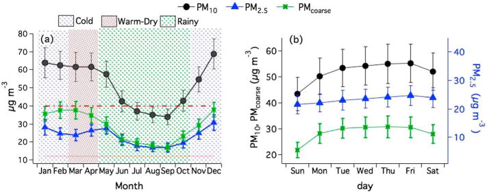
(a) Monthly and (b) weekly profiles of PM₁₀, PM_2.5, and PM_coarse from ground-based SIMAT station data between 2003 and 2015. The red horizontal lines in Figure 5a correspond to the Mexican guideline for PM₁₀ (40 μg m⁻³) and PM_2.5 (12 μg m⁻³). The whiskers represent one-fifth standard deviation.

PM₁₀ follows a weekly pattern pointing to some combination of accumulation of pollutants or increasing emissions during weekdays, leading to a peak around Thursday and Friday (55.0–55.3 μg m⁻³) and a minimum on Sunday (43.3 μg m⁻³; Figure 5b). Although PM_2.5 similarly peaks on Thursday and Friday (24.1–24.7 μg m⁻³) with a minimum on Sunday (21.6 μg m⁻³), the overall range of mean values on different days is small (~3 μg m⁻³) relative to PM₁₀ (~12 μg m⁻³) and PM_coarse (~9 μg m⁻³). PM_coarse exhibits its minimum value on Sunday (21.7 μg m⁻³) and shows similar values during weekdays (28.1–30.9 μg m⁻³). Potential signs of anthropogenic influence on temporal patterns of PM are discussed subsequently.

3.4. Surface Precipitation Data

Figure 6 shows the monthly profile of constituent concentrations in wet deposition in Mexico City between 2003 and 2015 based on SIMAT data, with no data in December any year. Sulfate and NO₃⁻ dominated in terms of aqueous-phase concentration, with peak levels between January and May and a second smaller peak in November. The next highest concentrations were for Ca²⁺ and NH₄⁺, which followed the same monthly profile as SO₄²⁻ and NO₃⁻. Accounting for much lower concentrations were Cl⁻, K⁺, Mg²⁺, and Na+.

Figure 6.

Monthly concentration profile of species in wet deposition from ground-based SIMAT station data between 2003 and 2015. No data were available for December in any year.

4. Discussion

4.1. Monthly Temporal Profiles

Other studies have shown that there are a range of factors that both govern the monthly profiles of columnar aerosol parameters (e.g., AOD and UV AI) and explain differences between columnar and surface PM data. It is pertinent to first note that the intercomparison between columnar spaceborne aerosol data and surface in situ measurements requires caution due to the different spatial fingerprints of the two types of data. When assuming that the intercomparison is fair to do, it was shown for the greater Tehran area [Crosbie et al., 2014] and South Africa [Hersey et al., 2015] that differences in temporal profiles between AOD and surface PM are due to lower PBLHs concentrating PM in a smaller volume of air leading to higher surface PM, whereas columnar AOD is immune to this issue. In our study region when PBLH is lowest (September–December), the surface PM concentrations exhibit the full range of levels including the minimum (September) and maximum (December) mean value for the entire year. Also, surface PM (PM₁₀, PM_2.5, and PM_coarse) levels are among their highest values when the PBLH is higher between March and May, concurrent with some of the higher values of columnar aerosol parameters (AOD and UV AI). The two moisture proxies in Figure 2 (water vapor and RH) are depressed between March and May, suggesting that aqueous processing to produce PM and aerosol swelling due to hygroscopic water uptake cannot explain the enhanced PM, AOD, and UV AI values during that time period.

The MAM months are shown to have more influence from air masses originating from the west as compared to other quarters (Figure 3), which can help point to why AOD and UV AI are highest in those months. Biomass burning is a stronger source of PM in the study region in the MAM months, which overlaps with the warm/dry season. Figure 7 shows the spatial distribution of fires by month in the study zone (Domain 1) between 2003 and 2015, with each red spot representing a 1 km grid cell. During the warm/dry months (March–April) and also May, more intense fires occur near coastal zones on both the western and eastern boundaries of the study domain. Over these areas the low deciduous forest, pine/oak forest, and high evergreen forest are the dominant types of vegetation (Figure 1b). During the cold/dry season (November–February), fire activity tends to be more intense in the central area of the spatial domain, especially next to Michoacan and Jalisco.

Figure 7.

Spatial frequency of monthly fires over central Mexico (the red-dotted rectangle corresponds to Domain 1 of Figure 1) based on MODIS FIRMS data between 2003 and 2015. The color is proportional to fire frequency (red = highest).

Figure 8 shows the monthly averages of brightness temperature (BT, proxy for fire intensity) and number of light spots between 2003 and 2015, with peak values in the MAM months. Conversely, the combination of the lowest frequency and intensity of fires occurs between August and October (i.e., during the rainy season). It is interesting that the total number of light spots (i.e., fires) occurs 1 month after the peak in BT. This may be explained by more numerous fires lacking intensity in May after the fires of April consume significant biomass fuel. Figures 7 and 8 help to support that biomass burning emissions contribute substantially to the high AOD, UV AI, and surface PM values between MAM when PBLH is highest. Soil dust can also contribute to enhancements of the aforementioned aerosol parameters and reductions in AE in the MAM months; Aiken et al. [2010] suggested that enhanced dust during periods of high biomass burning are due to independent emissions in the study region promoted by dry conditions rather than dust being lofted in the buoyant plumes of fires as shown in other regions [e.g., Maudlin et al., 2015].

Figure 8.

Monthly fire intensity (left axis) and total fire frequency (bottom right y axis) for central Mexico (Domain 1 of Figure 1) based on MODIS FIRMS data between 2003 and 2015. (top right y axis) Recalculated concentrations of PM_2.5, PM₁₀, and PM_coarse multiplied by average PBLH for a given month. The whiskers represent one standard deviation.

With regard to the surface PM concentration results (Figure 5), the reduction in the rainy season months of June–October is associated to a large extent with reduced biomass burning and increased wet scavenging (Figure 2a). High levels of surface PM in the colder months (November–February) are linked presumably to increased emissions from combustion for heating purposes. To remove the influence of PBLH between different months, Figure 8 repeats the results of Figure 5 except with the PM concentrations multiplied by the mean PBLH for each month. The recalculated concentrations follow the trend of BT more closely, peaking in the warm/dry season, providing support for regional biomass burning emissions in influencing both fine and coarse aerosol loadings in the study region. This result is in agreement with the recent study of Tzompa-Sosa et al. [2016].

Next we examine the monthly profile of speciated AOD contributions between 2003 to 2015 based on the GOCART model (Figure 9). The primary focus of the GOCART results is temporal monthly trends rather than relative absolute values owing to uncertainties associated with emissions inventories in the study region. Sulfate was found to have the largest AOD fraction, ranging from 0.065 to 0.1 with maximum values in May and June. Field measurements have shown that sulfate is not the most abundant species on a mass basis [e.g., Molina et al., 2007; Querol et al., 2008], which is suggestive of inaccurate emissions data used by the model. The comparable levels of SO₄²⁻ in September relative to the more fire-active months of May and June may be associated with the highest cloud fraction and columnar water vapor (Figure 2) and thus greatest potential for aqueous formation relative to other times of the year. While the current data set cannot quantify the relative contribution of different sources to SO₄²⁻ during different times of the year, its major sources are discussed. Major anthropogenic sources of SO₂ include fossil fuel combustion, industrial activity such as smelting, and biomass burning [Smith et al., 2011]. Additionally, volcanic emissions are a major source of sulfur emissions worldwide [Graf et al., 1997; Ge et al., 2016]. Two active volcanoes are located in the region: Colima, located 470 km west of Mexico City, and Popocatépetl, located 70 km southeast of Mexico City. Previous analysis of emissions from the Popocatépetl Volcano showed that the wind direction pointed northwest toward the MCMA for less than 20% of the analysis period [Grutter et al., 2008]. A previous analysis of SO₂ levels in the MCMA attributed a significant fraction of its emissions to local cement plants and industrial processes in the Tizayuca region [Almanza et al., 2014]. Other studies have demonstrated the impact of SO₂ emissions from the Tula Industrial Complex, located northwest of Mexico City [de Foy et al., 2007; Karydis et al., 2011; Ying et al., 2014].

Figure 9.

Monthly profile of speciated AOD from the Goddard Ozone Chemistry Aerosol Radiation and Transport (GOCART) model over central Mexico Megalopolis (Domain 2 of Figure 1) based on data between 2003 and 2015.

Organics exhibited a peak in April and May, overlapping with the period of strongest biomass burning influence (Figures 7 and 8). The optical depth associated with BC was similarly highest in April and May, consistent with more biomass burning emissions. Similar to BC, coarse dust AOD was also highest in April through June, both of which overlap with the highest UV AI values. Sea salt and fine dust have the smallest AOD values of the constituents studied, with their peaks also being between March–April and May, respectively.

An important source of aerosol, especially PM_2.5, is secondary production of aerosol from volatile organic compounds (VOCs) via gas-to-particle conversion. In a nearby region to the north in southern Arizona, it was shown that the combination of enhanced biogenic VOC emissions (as inferred from NDVI) and moisture between July and September resulted in significant SOA formation [Youn et al., 2013]. Figure 10 shows how NDVI is enhanced between July and October, overlapping with the wettest time of the year and enhanced plant growth as expected [Salinas-Zavala et al., 2002; Neeti et al., 2012] and thus biogenic emissions [Silveira and Oxana, 2014]. However, none of the aerosol parameters examined in this work exhibit any significant enhancement during this time period, which is an interesting finding by itself and worthy of more investigation. The current data set limits the discussion to presuming reasons as to why (i) the amount of other aerosol constituents (e.g., anthropogenic SOA) [Molina et al., 2007; Hennigan et al., 2008; Stone et al., 2008] outweighs that of SOA produced via biogenic emissions and thus cannot be observed with the data set used here; (ii) the amount of SOA produced is offset by wet scavenging during this portion of the year; and/or (iii) NDVI itself is not a fair proxy for biogenic emissions in the study region and future analyses focused on biogenic emissions should use other products.

Figure 10.

Monthly profiles of NDVI as retrieved from MODIS-Terra over Domain 1 shown in Figure 1 for the period between 2003 and 2015. The whiskers represent one standard deviation.

4.2. Influence of Anthropogenic Activity on PM

To extend upon Figure 5b where it was shown that PM, especially PM₁₀, was suppressed on weekends owing to less anthropogenic activity, here we examine how PM varied diurnally on weekdays and weekends (Figure 11). The diurnal PM₁₀ and PM_coarse profiles are similarly bimodal with a peak during the morning and evening rush hours (07:00–09:00 and 17:00–19:00). In contrast, PM_2.5 exhibits a unimodal profile with a dominant peak in the late morning (10:00–12:00). The data suggest that traffic results in some combination of resuspension of PM_coarse (e.g., road dust) and vehicular emissions enriched with PM_coarse. The source of PM_2.5 during the late morning may be associated with secondary production of aerosol via photochemistry as has been shown by others [Hennigan et al., 2008].

Figure 11.

Diurnal profile of (a) meteorological parameters and (b) PM₁₀, (c) PM_2.5, and (d) PM_coarse from ground-based SIMAT station data between 2003 and 2015. Figures 11b–11d report profiles for all data (cumulative), weekdays only, and weekend days only (Saturday–Sunday) with whiskers representing one-fifth of standard deviation.

The diurnal profiles of key meteorological parameters are summarized in Figure 11a to help interpret the PM data. It is shown that RH is highest at around 06:00 (71%) and lowest at 14:00 (32%), which alone cannot help explain any of the PM diurnal profiles. Moisture promotes production of secondary inorganic (e.g., ammonium nitrate) and organic species, as evident in other megacities such as Los Angeles [Hersey et al., 2011; Ryerson et al., 2013]. Earlier studies [e.g., Hennigan et al., 2008] showed that ammonium nitrate dominated the inorganic aerosol fraction in Mexico City with rapid morning production and a peak near 11:00, followed by a rapid midday reduction in concentration owing to boundary layer deepening (and thus dilution) and, to a lesser extent, volatilization. They also showed similar temporal characteristics for water-soluble organic carbon, which is also mainly produced via a secondary formation mechanism in Mexico City. Approximately 75% of the morning concentration increases were said to be due to secondary formation in that study. Figure 11 shows that temperature exhibits its highest levels between 11:00 and 15:00, which is just after PM_2.5 peaks at 10:00. Thus, it is likely that secondary production of aerosol species contributes to the growth in the PM_2.5 profile in the morning, and the subsequent reduction can be linked to higher temperatures, concurrent with more volatilization of aerosol, and a deepening boundary layer that dilutes its concentrations. The precursor emissions leading to the secondary aerosol have been noted to mainly be from anthropogenic sources [e.g., Molina et al., 2007; Hennigan et al., 2008], especially vehicular emissions [Velasco et al., 2007], in the study region. Wind speed does not follow the temporal profile of any of the PM species and thus is ruled out as a key driver of diurnal PM profiles in the study region.

Figures 11b–11d show diurnal profiles for weekends and weekdays. A clear anthropogenic signature is evident with higher levels of PM on weekdays at all times of the day except from ~00:00 to 06:00. The “weekday-weekend” difference for PM₁₀ followed the same bimodal profile as the cumulative PM₁₀ temporal profile in Figure 11b, with maximum values of the difference being around the two rush hours: 07:00 = 16.1 μg m⁻³ and 18:00 = 11.5 μg m⁻³. Expectedly, the same characteristics apply to PM_coarse with its maximum difference values being during the rush hours: 07:00 = 14.0 μg m⁻³ and 18:00 = 10.1 μg m⁻³. For PM_2.5 the differences between weekends and weekdays were less severe, with the maximum values being between 06:00 and 13:00 (1.2–2.3 μg m⁻³) and the peak at 08:00. These results indicate that an anthropogenic effect during the vehicular rush hours accounts for a significant amount of PM_coarse emissions (i.e., primary anthropogenic aerosol) and, to a lesser extent, PM_2.5. The source of these particles in the PM_coarse fraction is most likely primary particles unrelated to engines such as resuspended dust.

4.3. Interrelationships Between Precipitation and Aerosol Species

Table 3 displays the correlation matrix between major soluble ions in precipitation and surface PM₁₀ and PM_2.5, based on monthly averaged SIMAT data for the period between 2003 and 2015. Correlations discussed here and reported in Table 3 are statistically significant based on 95% confidence using a twotailed Student’s t test. We note that while the correlations are not proof for causation, they can still be used to speculate as to what major sources impact precipitation chemistry in the study region. The two mechanisms by which the subsequently discussed species could partition to rainwater are either via aerosol scavenging of these species (i.e., activation into drops) or by their gaseous precursors (if they exist, such as HNO₃ for NO₃⁻) transferring into the aqueous phase [Van der Swaluw et al., 2011].

Table 3.

Correlation Matrix Between Major Rainwater Ionic Constituents and Surface PM₁₀ and PM_2.5 Between 2003 and 2015^a

	Ca2+: Rain	NO3− : Rain	NH4+: Rain	Na+: Rain	Mg2+: Rain	K+: Rain	Cl− : Rain	SO42− -: Rain	PM2.5	PM10	PMcoarse
Ca2+: rain		78	78	78	78	78	78	78	73	78	73
NO3−: rain	0.71		78	78	78	78	78	78	73	78	73
NH4+: rain	0.81	0.81		78	78	78	78	78	73	78	73
Na+: rain	0.34	0.44	0.39		78	78	78	78	73	78	73
Mg2+: rain	0.52	0.56	0.59	0.56		78	78	78	73	78	73
K+: rain	0.56	0.67	0.74	0.51	0.76		78	78	73	78	73
Cl−: rain	0.34	0.57	0.42	0.37	0.38	0.50		78	73	78
SO42−-: rain	0.68	0.80	0.85	0.47	0.64	0.79	0.47		73	78	73
PM2.5	0.74	0.63	0.79	0.32	0.51	0.62	0.41	0.72		140	140
PM10	0.85	0.66	0.84	0.37	0.54	0.63	0.31	0.75	0.89		140
PMcoarse		0.80	0.59	0.75	0.37	0.58	0.55	0.66	0.97	0.75

^aThe analysis is based on data collected during periods with coincident precipitation and PM measurements at Mexico City SIMAT stations. The lower left triangular matrix displays r values for the correlations, while the upper right triangular matrix displays the number of samples (n) for each respective correlation.

PM₁₀ and PM_coarse exhibit their highest correlations with NH₄⁺, SO₄²⁻, NO₃⁻, and Ca²⁺. As the highest correlation of PM₁₀ and PM_coarse was with the dust tracer Ca²⁺, dust presumably plays a significant role in seeding the precipitation drops in the study region. A similar result has been shown for the Sonoran Desert to the north of the Mexico border by southern Arizona [Sorooshian et al., 2013]. This latter study suggested that the secondary inorganic species (NH₄⁺, SO₄²⁻, and NO₃⁻) in wet deposition were correlated with fine soil levels owing likely to partitioning of these species onto coarse aerosol surfaces; it is plausible that the same explanation could apply to the study region. The data suggest that sea salt is not a major source for Cl⁻ and Na⁺ in precipitation because both species exhibit the weakest correlations with PM₁₀ and PM_coarse, and additionally, the relation between Cl⁻ and Na+ is not very strong (r = 0.37, n = 78).

PM_2.5 was best correlated with NH₄⁺, SO₄²⁻, and Ca²⁺ (r = 0.72–0.79, n = 73) among the eight wet deposition constituents examined. This is suggestive of these three constituents being important components of the particles seeding precipitation drops. The precipitation species with the lowest correlation with PM_2.5 included Cl⁻ and Na⁺, indicative of little influence from fine sea salt particles. Previous studies in the area have shown a link between garbage burning and emissions of Cl⁻ and PM_2.5 in the MCMA [Li et al., 2012; Hodzic et al., 2012], which may partly help explain the peculiar correlation results for Cl⁻ where it is not correlated with Na⁺. Li et al. [2012] found that Cl⁻ contributed a significant fraction (10%) of the PM_2.5 mass emitted through garbage burning in the MCMA.

In terms of interrelationships among precipitation species, SO₄²⁻ and NH₄⁺ exhibited the highest correlation (r = 0.85, n = 78), suggestive of influence from anthropogenic sources leading to their gaseous precursors (SO₂ and NH₃, respectively). In addition, NO₃⁻ and SO₄²⁻ exhibited good correlation (r = 0.80, n = 78), in agreement with Dias et al. [2012]. Ammonium and SO₄²⁻ often exhibit the same mass size distribution with peaks in the accumulation mode, indicative of secondary formation via acid-base chemistry [e.g., Maudlin et al., 2015; Youn et al., 2015]. Sources of NH₃ include livestock waste, fertilizer, biomass burning, and vehicular emissions [Battye et al., 2003].

Some of the next strongest correlations are between NO₃⁻ and either SO₄²⁻ (r = 0.80, n = 78) or NH₄⁺ (r = 0.81, n = 78). Nitrate’s main precursor, nitric acid (formed from NO_x emissions), participates in acid-base chemistry with NH₃ and other bases such as amines to form NO₃⁻ salts, analogous to the process by which sulfuric acid forms SO₄²⁻ salts. Ammonium sulfate production is thermodynamically more favorable as compared to ammonium nitrate, which is why NO₃⁻ is thought to partition more effectively to the aerosol phase once SO₄²⁻ is fully neutralized [e.g., Stelson et al., 1979]. The main source of NO_x in Mexico City is mobile emissions [Karydis et al., 2011], with other major sources including biomass burning and industrial activity [Garg et al., 2001; Reis et al., 2009]. Other studies in the region have shown that these three species, representing the major secondary inorganic aerosol species in the study region, are fairly similar in concentration with a regional character owing to their homogeneity, but with enhancements near major industrial/urban sources [e.g., Salcedo et al., 2006; Querol et al., 2008].

The five species that typically are associated with coarse matter such as sea salt or crustal particles (i.e., Ca⁺², Na⁺, Cl⁻, Mg⁺², and K⁺) exhibit significant correlations with one another (r = 0.34–0.76, n = 78). The dry Texcoco Lake bed to the east of Mexico City is a noteworthy source of these species [Karydis et al., 2011]. These five species, however, exhibit comparable or even higher correlations with NO₃⁻, SO₄²⁻, and NH₄⁺ than among each other. For example, Ca²⁺ exhibits correlation coefficients between 0.68 and 0.81 with NO₃⁻, SO₄²⁻, and NH₄⁺, while it exhibits values between 0.34 and 0.56 with Na⁺, Mg²⁺, K⁺, and Cl⁻. There are at least two explanations for this result: (i) reactions of acids (e.g., nitric and sulfuric acids) with coarse aerosol surfaces (most likely dust), which has been documented for other regions such as southwestern parts of the United States [Sorooshian et al., 2011, 2013], India [Satyanarayana et al., 2010], and by the California coastal zone [Prabhakar et al., 2014], and (ii) Ca²⁺, Na⁺, Cl⁻, Mg²⁺, and K⁺ could be major components in PM_2.5 (and do not stem mainly from coarse particle types such as dust and sea salt) and can become internally mixed with particles enriched with NO₃⁻, SO₄²⁻, and NH₄⁺. For example, one possible source of Ca²⁺ is cement plants, which, during a study in Spain, were linked to increased levels of Ca²⁺ in PM_2.5 [Galindo et al., 2011]. Other point sources, such as garbage burning, could account for the strong correlations of Ca²⁺, Na⁺, Cl⁻, Mg²⁺, and K⁺ with NO₃⁻, SO₄²⁻, and NH₄⁺ in PM_2.5 but weaker correlations among one another.

4.4. Interannual Trends

Table 4 presents a summary of how PM species (PM₁₀, PM_2.5, and PM_coarse) and wet deposition have changed between 2003 and 2015 as a function of season. For PM₁₀, PM_2.5, and PM_coarse, concentrations have generally decreased over time based on the slopes of best fit lines; the P-values using a two-tailed Student’s t test indicate that the PM trends are not statistically significant with a P-value threshold of 0.15 for any annual quarter shown. It is worth noting though that the lowest slopes were for the JJA months and the highest ones were for MAM and DJF.

Table 4.

Interannual Trend Analysis Results for Wet Deposition Species and Surface PM₁₀, PM_2.5, and PM_coarse Between 2003 and 2015 as a Function of Annual Quarters Based On SIMAT Data^a

	r2	DJF		r2	MAM		r2	JJA		r2	SON
		Slope	P-value		Slope	P-value		Slope	P-value		Slope	P-value
PM10	0.01	−0.37	0.52	0.02	−0.45	0.37	0.00	−0.07	0.80	0.00	−0.19	0.74
PM2.5	0.06	−0.35	0.16	0.04	−0.24	0.27	0.00	0.03	0.82	0.03	−0.21	0.30
PMcoarse	0.00	−0.02	0.96	0.01	−0.21	0.58	0.01	−0.10	0.63	0.00	0.03	0.94
Ca2+: rain	–	–	–	0.04	−0.08	0.49	0.01	−0.01	0.51	0.07	−0.07	0.23
Cl− : rain	–	–	–	0.18	−0.04	0.13	0.00	0.00	0.80	0.00	0.00	0.80
K+ : rain	–	–	–	0.11	−0.04	0.24	0.10	−0.01	0.06	0.10	−0.01	0.12
Mg2+ : rain	–	–	–	0.35	−0.03	0.02	0.11	−0.01	0.05	0.13	−0.01	0.07
Na+ : rain	–	–	–	0.24	−0.03	0.08	0.00	0.00	0.93	0.01	0.00	0.60
NH4+ : rain	–	–	–	0.13	−0.11	0.20	0.10	−0.05	0.05	0.08	−0.06	0.18
NO3− : rain	–	–	–	0.09	−0.25	0.30	0.00	0.00	0.99	0.04	−0.15	0.35
SO42− : rain	–	–	–	0.09	−0.21	0.29	0.01	−0.03	0.66	0.01	0.05	0.62

^aSlopes correspond to units of μg m ⁻³ y ⁻¹ for PM species and mg L ⁻¹ y⁻¹ for wet deposition species. The correlation coefficients (r²) and P-values correspond to the line of best fit. No wet deposition data were available for the DJF quarter.

The wet deposition species concentrations also generally exhibited negative slopes but with lower P-values, indicative of more statistical significance in the trend over time. Of all wet deposition species, Mg²⁺ exhibited the lowest P-values (0.02–0.07) with slopes ranging from −0.01 to −0.03 mg L⁻¹ y⁻¹. In the MAM months, Na⁺ exhibited the next most statistically significant reduction (−0.03 mg L⁻¹ y⁻¹; P-value = 0.08). In MAM, SO₄²⁻ and NO₃⁻ exhibited the highest slope of any species in any annual quarter, albeit in the negative direction (−0.21 and −0.25 mg L⁻¹ y⁻¹, respectively). Lastly, K⁺ also exhibited reductions in JJA (−0.01 mg L⁻¹ y⁻¹) and SON (−0.01 mg L⁻¹ y ⁻¹) with P-values (0.06–0.12) exceeding most other species. Of relevance to air quality, the interannual profiles of fire-related parameters are evaluated. Figure 12 reports the interannual variation in average and maximum BT and total number of light spots. The highest values for number of light spots were observed in 2005, 2011, and 2013, while the lowest values were in the most recent years of 2014 and 2015. Although fire frequency varies annually, fire intensity (i.e., BT) remains mostly constant, with the mean annual BT usually being ~327 K. It is interesting that slightly lower values have been observed in 2014–2015 (325.5–325.7 K). The maximum intensity of fires, based on BT values, does not exhibit any relationship with mean BT or light spots and varied between 429 and 500 K. Thus, the fire data do not reveal a clear trend since 2002 other than an interesting reduction in mean BT and light spots in 2014–2015, which warrants additional investigation as to whether this trend continues in upcoming years.

Figure 12.

Interannual profile of light spot frequency and brightness temperature (BT) for central Mexico (Domain 1 of Figure 1). The maximum and standard deviation (divided by 5) of BT is also shown for each year.

A natural question arises as to whether air quality improved in 2014 and 2015 as compared to earlier years owing to reduced fire activity. Figure S1 in the supporting information further shows changes in PM_2.5, PM₁₀, and PM_coarse for the period between before and after the start of 2014, further confirming the reductions in PM_2.5, PM₁₀, and PM_coarse specifically for the latter two parameters. Therefore, even though statistically significant improvements in surface PM levels were not observed during the study period as a result of regulatory policies, a noticeable improvement occurred coincident with reduced biomass burning in the region. Interestingly, more reductions were observed in PM_coarse as compared to PM_2.5, which motivates more research to identify what the source is of those larger particles and how much of it can be accounted for by soil dust and other primary particles advected within fire plumes.

5. Conclusions

This study presents a 13 year comprehensive analysis of aerosol characteristics over the Megalopolis of Central Mexico region, using remotely sensed data, ground-based in situ measurements, and modeling. The results of this study are as follows following the order of questions posed at the end of section 1:

1. The highest values of AOD and UV AI are observed between March and May, when PBLH is high and surface PM (PM₁₀, PM_2.5, and PM_coarse) concentrations are also enhanced relative to most other months. Analysis reveals that a major contributor to the pollution in those months is biomass burning, especially near coastal zones to the west of the country, an area that is mainly covered by low deciduous forest, pine/oak forest, and high evergreen forest. The reduction of PM and remotely sensed AOD values during the rainy season months is associated with reduced biomass burning and increased wet scavenging.

2. Weekly analysis reveals the lowest values of PM on weekends with an even clearer anthropogenic signature evident when examining differences in diurnal profiles between weekend and weekdays. A striking result is the sharp enhancement of PM_coarse during the two rush hours on weekdays relative to weekends owing to nonengine-related vehicular traffic emissions such as dust resuspension. The difference between weekends and weekdays was less prominent for PM_2.5.

3. Intercomparison of surface PM and wet deposition chemistry data suggests that NH₄⁺, SO₄²⁻, and Ca²⁺ are important components of the aerosol seeding the precipitation drops that eventually fall as wet deposition in the Megalopolis. Dust in particular is likely an active agent in leading to enhanced Ca²⁺ levels in precipitation. In contrast, Cl⁻ and Na⁺ were the two wet deposition species exhibiting the weakest relationship with PM levels.

4. Interannual analysis between 2003 and 2015 of PM concentrations shows that trends are not statistically significant at 95% confidence. Of note though is that PM concentration reductions were observed for 2014–2015 owing to reduced regional biomass burning as compared to 2003–2013 during the warm-dry season.

Key Points.

• Reductions in surface particulate matter were observed in 2014–2015 (versus 2003–2013) owing to reduced regional fire activity

• Primary emissions, such as resuspended dust, result in enhanced aerosol mass concentrations during most of the diurnal cycle on weekdays versus weekend days

• Among wet deposition species, NH4⁺, SO₄²⁻, and Ca²⁺ are best correlated with PM_2.5 and PM₁₀

References

- Adachi K, Buseck PR. Internally mixed soot, sulfates, and organic matter in aerosol particles from Mexico City. Atmos Chem Phys. 2008;8(21):6469–6481. doi: 10.5194/acp-8-6469-2008. [DOI] [Google Scholar]
- Aiken AC, et al. Mexico City aerosol analysis during MILAGRO using high resolution aerosol mass spectrometry at the urban supersite (T0)—Part 1: Fine particle composition and organic source apportionment. Atmos Chem Phys. 2009;9(17):6633–6653. [Google Scholar]
- Aiken AC, et al. Mexico City aerosol analysis during MILAGRO using high resolution aerosol mass spectrometry at the urban supersite (T0)—Part 2: Analysis of the biomass burning contribution and the non-fossil carbon fraction. Atmos Chem Phys. 2010;70(12):5315–5341. doi: 10.5194/acp-10-5315-2010. [DOI] [Google Scholar]
- Almanza VH, Molina LT, Sosa G. Soot and SO2 contribution to the supersites in the MILAGRO campaign from elevated flares in the Tula refinery. Atmos Chem Phys. 2012;12(21):10,583–10,599. doi: 10.5194/acp-12-10583-2012. [DOI] [Google Scholar]
- Almanza VH, Molina LT, Li G, Fast J, Sosa G. Impact of external industrial sources on the regional and local SO2 and O-3 levels of the Mexico megacity. Atmos Chem Phys. 2014;14(16):8483–8499. doi: 10.5194/acp-14-8483-2014. [DOI] [Google Scholar]
- Andres RJ, Kasgnoc AD. A time-averaged inventory of subaerial volcanic sulfur emissions. J Geophys Res. 1998;103(D19):25,251–25,261. doi: 10.1029/98JD02091. [DOI] [Google Scholar]
- Battye W, V, Aneja P, Roelle PA. Evaluation and improvement of ammonia emissions inventories. Atmos Environ. 2003;37(27):3873–3883. doi: 10.1016/S1352-2310(03)00343-1. [DOI] [Google Scholar]
- Bhandari AK, Kumar A. Feature extraction using normalized difference vegetation index (NDVI): A case study of Jabalpur City, proceedings of communication, computing & security. Proced Tech. 2012;6:612–621. [Google Scholar]
- Bravo AH, Sosa ER, Sanchez AP, Jaimes PM, Saavedra RMI. Impact of wildfires on the air quality of Mexico City, 1992–1999. Environ Pollut. 2002;117(2):243–253. doi: 10.1016/S0269-7491(01)00277-9. [DOI] [PubMed] [Google Scholar]
- Carreon-Sierra S, Salcido A, Castro T, Celada-Murillo AT. Cluster analysis of the wind events and seasonal wind circulation patterns in the Mexico City region. Atmos Basel. 2015;6(8):1006–1031. doi: 10.3390/atmos6081006. [DOI] [Google Scholar]
- Chin M, Ginoux P, Kinne S, Torres O, Holben BN, Duncan BN, Martin RV, Logan JA, Higurashi A, Nakajima T. Tropospheric aerosol optical thickness from the GOCART model and comparisons with satellite and Sun photometer measurements. J Atmos Sci. 2002;59(3):461–483. doi: 10.1175/1520-0469(2002)059<0461:Taotft>2.0.Co;2. [DOI] [Google Scholar]
- Chin M, et al. Multi-decadal aerosol variations from 1980 to 2009:A perspective from observations and a global model. Atmos Chem Phys. 2014;14(7):3657–3690. doi: 10.5194/acp-14-3657-2014. [DOI] [Google Scholar]
- Cook ER, Meko DM, Stahle DW, Cleaveland MK. Drought reconstructions for the continental United States. J Clim. 1999;12(4):1145–1162. doi: 10.1175/1520-0442(1999)012<1145:Drftcu>2.0.Co;2. [DOI] [Google Scholar]
- Crosbie E, Sorooshian A, Monfared NA, Shingler T, Esmaili O. A multi-year aerosol characterization for the greater Tehran area using satellite, surface, and modeling data. Atmos Basel. 2014;5(2):178–197. doi: 10.3390/atmos5020178. [DOI] [PMC free article] [PubMed] [Google Scholar]
- de Foy B, Caetano E, Magana V, Zitacuaro A, Cardenas B, Retama A, Ramos R, Molina LT, Molina MJ. Mexico City basin wind circulation during the MCMA-2003 field campaign. Atmos Chem Phys. 2005;5:2267–2288. [Google Scholar]
- de Foy B, Varela JR, Molina LT, Molina MJ. Rapid ventilation of the Mexico City basin and regional fate of the urban plume. Atmos Chem Phys. 2006;6:2321–2335. [Google Scholar]
- de Foy B, et al. Modelling constraints on the emission inventory and on vertical dispersion for CO and SO2 in the Mexico City Metropolitan Area using solar FTIR and zenith sky UV spectroscopy. Atmos Chem Phys. 2007;7:781–801. [Google Scholar]
- de Foy B, Krotkov NA, Bei N, Herndon SC, Huey LG, Martinez AP, Ruiz-Suarez LG, Wood EC, Zavala M, Molina LT. Hit from both sides: Tracking industrial and volcanic plumes in Mexico City with surface measurements and OMI SO2 retrievals during the MILAGRO field campaign. Atmos Chem Phys. 2009;9(24):9599–9617. doi: 10.5194/acp-9-9599-2009. [DOI] [Google Scholar]
- de Foy B, Burton SP, Ferrare RA, Hostetler CA, Hair JW, Wiedinmyer C, Molina LT. Aerosol plume transport and transformation in high spectral resolution lidar measurements and WRF-Flexpart simulations during the MILAGRO field campaign. Atmos Chem Phys. 2011;11(7):3543–3563. doi: 10.5194/acp-11-3543-2011. [DOI] [Google Scholar]
- Dias VRD, Sanches L, Alves MD, Nogueira JD. Spatio-temporal variability of anions in wet precipitation of Cuiaba, Brazil. Atmos Res. 2012;107:9–19. doi: 10.1016/j.atmosres.2011.11.003. [DOI] [Google Scholar]
- Diner DJ, Hansen E. Tech Rep. Jet Propulsion Laboratory, California Institute of Technology; 2012. Multi-Angle Imaging Spectroradiometer (MISR): Data product specification for the MISR level 3. Joint aerosol product. [Google Scholar]
- Duncan BN, Martin RV, Staudt AC, Yevich R, Logan JA. Interannual and seasonal variability of biomass burning emissions constrained by satellite observations. J Geophys Res. 2003;108(D2):4040. doi: 10.1029/2002JD002378. [DOI] [Google Scholar]
- Galindo N, Yubero E, Nicolas JF, Crespo J, Pastor C, Carratala A, Santacatalina M. Water-soluble ions measured in fine particulate matter next to cement works. Atmos Environ. 2011;45(12):2043–2049. doi: 10.1016/j.atmosenv.2011.01.059. [DOI] [Google Scholar]
- Garg A, Shukla PR, Bhattacharya S, Dadhwal VK. Sub-region (district) and sector level SO2 and NOx emissions for India: Assessment of inventories and mitigation flexibility. Atmos Environ. 2001;35(4):703–713. doi: 10.1016/S1352-2310(00)00316-2. [DOI] [Google Scholar]
- Ge C, Wang J, Carn S, Yang K, Ginoux P, Krotkov N. Satellite-based global volcanic SO2 emissions and sulfate direct radiative forcing during 2005-2012. J Geophys Res Atmos. 2016;121:3446–3464. doi: 10.1002/2015JD023134. [DOI] [Google Scholar]
- Giglio L, Schroeder W, Justice CO. The collection 6 MODIS active fire detection algorithm and fire products. Remote Sens Environ. 2016;178:31–41. doi: 10.1016/j.rse.2016.02.054. [DOI] [PMC free article] [PubMed] [Google Scholar]
- Graf HF, Feichter J, Langmann B. Volcanic sulfur emissions: Estimates of source strength and its contribution to the global sulfate distribution. J Geophys Res. 1997;102(D9):10,727–10,738. doi: 10.1029/96JD03265. [DOI] [Google Scholar]
- Grutter M, Basaldud R, Rivera C, Harig R, Junkerman W, Caetano E, Delgado-Granados H. SO2 emissions from Popocatepetl volcano: Emission rates and plume imaging using optical remote sensing techniques. Atmos Chem Phys. 2008;8(22):6655–6663. [Google Scholar]
- Helfand HM, Labraga JC. Design of a nonsingular level 2.5 2nd-order closure-model for the prediction of atmospheric-turbulence. J Atmos Sci. 1988;45(2):113–132. doi: 10.1175/1520-0469(1988)045<0113:Doanls>2.0.Co;2. [DOI] [Google Scholar]
- Hennigan CJ, et al. On the volatility and production mechanisms of newly formed nitrate and water soluble organic aerosol in Mexico City. Atmos Chem Phys. 2008;8(14):3761–3768. [Google Scholar]
- Hersey SP, Craven JS, Schilling KA, Metcalf AR, Sorooshian A, Chan MN, Flagan RC, Seinfeld JH. The Pasadena Aerosol Characterization Observatory (PACO): Chemical and physical analysis of the western Los Angeles basin aerosol. Atmos Chem Phys. 2011;11(15):7417–7443. doi: 10.5194/acp-11-7417-2011. [DOI] [Google Scholar]
- Hersey SP, Garland RM, Crosbie E, Shingler T, Sorooshian A, Piketh S, Burger R. An overview of regional and local characteristics of aerosols in South Africa using satellite, ground, and modeling data. Atmos Chem Phys. 2015;15(8):4259–4278. doi: 10.5194/acp-15-4259-2015. [DOI] [PMC free article] [PubMed] [Google Scholar]
- Hodzic A, Wiedinmyer C, Salcedo D, Jimenez JL. Impact of trash burning on air quality in Mexico City. Environ Sci Technol. 2012;46(9):4950–4957. doi: 10.1021/es203954r. [DOI] [PubMed] [Google Scholar]
- Holben BN, et al. AERONET—A federated instrument network and data archive for aerosol characterization. Remote Sens Environ. 1998;66(1):1–16. doi: 10.1016/S0034-4257(98)00031-5. [DOI] [Google Scholar]
- Hsu NC, Tsay SC, King MD, Herman JR. Aerosol properties over bright-reflecting source regions. IEEE Trans Geosci Remote Sens. 2004;42(3):557–569. doi: 10.1109/Tgrs.2004.824067. [DOI] [Google Scholar]
- Hsu NC, Jeong MJ, Bettenhausen C, Sayer AM, Hansell R, Seftor CS, Huang J, Tsay SC. Enhanced deep blue aerosol retrieval algorithm: The second generation. J Geophys Res Atmos. 2013;118:9296–9315. doi: 10.1002/jgrd.50712. [DOI] [Google Scholar]
- Jauregui E. Heat island development in Mexico City. Atmos Environ. 1997;31(22):3821–3831. doi: 10.1016/S1352-2310(97)00136-2. [DOI] [Google Scholar]
- Jorba O, Perez C, Rocadenbosch F, Baldasano JM. Cluster analysis of 4-day back trajectories arriving in the Barcelona area. Spain, from 1997 to 2002. J Appl Meteorol. 2004;43(6):887–901. doi: 10.1175/1520-0450(2004)043<0887:Caodbt>2.0.Co;2. [DOI] [Google Scholar]
- Kahn RA, Gaitley BJ, Martonchik JV, Diner DJ, Crean KA, Holben B. Multiangle Imaging Spectroradiometer (MISR) global aerosol optical depth validation based on 2 years of coincident Aerosol Robotic Network (AERONET) observations. J Geophys Res. 2005;110:D10S04. doi: 10.1029/2004JD004706. [DOI] [Google Scholar]
- Kahn RA, Gaitley BJ, Garay MJ, Diner DJ, Eck TF, Smirnov A, Holben BN. Multiangle Imaging Spectroradiometer global aerosol product assessment by comparison with the Aerosol Robotic Network. J Geophys Res. 2010;115:D23209. doi: 10.1029/2010JD014601. [DOI] [Google Scholar]
- Kar J, Vaughan MA, Liu Z, Omar AH, Trepte CR, Tackett J, Fairlie TD, Kowch R. Detection of pollution outflow from Mexico City using CALIPSO lidar measurements. Remote Sens Environ. 2015;169:205–211. doi: 10.1016/j.rse.2015.08.009. [DOI] [Google Scholar]
- Karydis VA, Tsimpidi AP, Lei W, Molina LT, Pandis SN. Formation of semivolatile inorganic aerosols in the Mexico City Metropolitan Area during the MILAGRO campaign. Atmos Chem Phys. 2011;11(24):13,305–13,323. doi: 10.5194/acp-11-13305-2011. [DOI] [Google Scholar]
- Klaus D, Jauregui E, Poth A, Stein G, Voss M. Regular circulation structures in the tropical basin of Mexico City as a consequence of the urban heat island effect. Erdkunde. 1999;53:231–243. [Google Scholar]
- Levy RC, Mattoo S, Munchak LA, Remer LA, Sayer AM, Patadia F, Hsu NC. The collection 6 MODIS aerosol products over land and ocean. Atmos Meas Tech. 2013;6(11):2989–3034. doi: 10.5194/amt-6-2989-2013. [DOI] [Google Scholar]
- Li G, Lei W, Bei N, Molina LT. Contribution of garbage burning to chloride and PM2.5 in Mexico City. Atmos Chem Phys. 2012;12(18):8751–8761. doi: 10.5194/acp-12-8751-2012. [DOI] [Google Scholar]
- Li J, Carlson BE, Lacis AA. Application of spectral analysis techniques in the intercomparison of aerosol data: 1. An EOF approach to analyze the spatial-temporal variability of aerosol optical depth using multiple remote sensing data sets. J Geophys Res Atmos. 2013;118:8640–8648. doi: 10.1002/jgrd.50686. [DOI] [Google Scholar]
- Li J, Carlson BE, Lacis AA. Application of spectral analysis techniques in the intercomparison of aerosol data. Part II: Using maximum covariance analysis to effectively compare spatiotemporal variability of satellite and AERONET measured aerosol optical depth. J Geophys Res Atmos. 2014a;119:153–166. doi: 10.1002/2013JD020537. [DOI] [Google Scholar]
- Li J, Carlson BE, Lacis AA. Application of spectral analysis techniques in the intercomparison of aerosol data: Part III. Using combined PCA to compare spatiotemporal variability of MODIS, MISR, and OMI aerosol optical depth. J Geophys Res Atmos. 2014b;119:4017–4042. doi: 10.1002/2013JD020538. [DOI] [Google Scholar]
- Li J, Carlson BE, Lacis AA. How well do satellite AOD observations represent the spatial and temporal variability of PM2.5 concentration for the United States? Atmos Environ. 2015;102:260–273. doi: 10.1016/j.atmosenv.2014.12.010. [DOI] [Google Scholar]
- Li Z, Zhao X, Kahn R, Mishchenko M, Remer L, Lee KH, Wang M, Laszlo I, Nakajima T, Maring H. Uncertainties in satellite remote sensing of aerosols and impact on monitoring its long-term trend: A review and perspective. Ann Geophys. 2009;27(7):2755–2770. [Google Scholar]
- Lin SJ, Rood RB. Multidimensional flux-form semi-Lagrangian transport schemes. Mon Weather Rev. 1996;124(9):2046–2070. doi: 10.1175/1520-0493(1996)124<2046:Mffslt>2.0.Co;2. [DOI] [Google Scholar]
- Livingston JM, et al. Comparison of aerosol optical depths from the Ozone Monitoring Instrument (OMI) on Aura with results from airborne sunphotometry, other space and ground measurements during MILAGRO/INTEX-B. Atmos Chem Phys. 2009;9(18):6743–6765. [Google Scholar]
- Lopez DH, et al. Frequency and character of extreme aerosol events in the southwestern United States: A case study analysis in Arizona. Atmos Basel. 2016;7(1) doi: 10.3390/atmos7010001. [DOI] [PMC free article] [PubMed] [Google Scholar]
- Maudlin LC, Wang Z, Jonsson HH, Sorooshian A. Impact of wildfires on size-resolved aerosol composition at a coastal California site. Atmos Environ. 2015;119:59–68. doi: 10.1016/j.atmosenv.2015.08.039. [DOI] [Google Scholar]
- Molina LT, et al. Air quality in North America’s most populous city—Overview of the MCMA-2003 campaign. Atmos Chem Phys. 2007;7(10):2447–2473. [Google Scholar]
- Molina LT, et al. An overview of the MILAGRO 2006 campaign: Mexico City emissions and their transport and transformation. Atmos Chem Phys. 2010;10(18):8697–8760. doi: 10.5194/acp-10-8697-2010. [DOI] [Google Scholar]
- Neeti N, Rogan J, Christman Z, Eastman JR, Millones M, Schneider L, Nickl E, Schmook B, Turner BL, Ghimire B. Mapping seasonal trends in vegetation using AVHRR-NDVI time series in the Yucatan Peninsula, Mexico. Remote Sens Lett. 2012;3:433–442. [Google Scholar]
- Olivier JGJ, et al. Description of EDGAR version 2.0: A set of global emission inventories of greenhous gases and ozone-depleting substances for all anthropogenic and most natural sources on a per country basis and on 1 × 1 grid. National Institute of Public Health and the Environment (RIVM) report no. 771060 002/TNO-MEP Report no. R96/119 1996 [Google Scholar]
- Ostby TI, Schuler TV, Westermann S. Severe cloud contamination of MODIS land surface temperatures over an Arctic ice cap, Svalbard. Remote Sens Environ. 2014;142:95–102. doi: 10.1016/j.rse.2013.11.005. [DOI] [Google Scholar]
- Perez-Ramirez D, Whiteman DN, Smirnov A, Lyamani H, Holben BN, Pinker R, Andrade M, Alados-Arboledas L. Evaluation of AERONET precipitable water vapor versus microwave radiometry, GPS, and radiosondes at ARM sites. J Geophys Res Atmos. 2014;119:9596–9613. doi: 10.1002/2014JD021730. [DOI] [Google Scholar]
- Prabhakar G, Ervens B, Wang Z, Maudlin LC, Coggon MM, Jonsson HH, Seinfeld JH, Sorooshian A. Sources of nitrate in stratocumulus cloud water: Airborne measurements during the 2011 E-PEACE and 2013 NiCE studies. Atmos Environ. 2014;97:166–173. doi: 10.1016/j.atmosenv.2014.08.019. [DOI] [Google Scholar]
- Querol X, et al. PM speciation and sources in Mexico during the MILAGRO-2006 campaign. Atmos Chem Phys. 2008;8(1):111–128. doi: 10.5194/acp-8-111-2008. [DOI] [Google Scholar]
- Redemann J, Zhang Q, Livingston J, Russell P, Shinozuka Y, Clarke A, Johnson R, Levy R. Testing aerosol properties in MODIS collection 4 and 5 using airborne sunphotometer observations in INTEX-B/MILAGRO. Atmos Chem Phys. 2009;9(21):8159–8172. [Google Scholar]
- Reis S, Pinder RW, Zhang M, Lijie G, Sutton MA. Reactive nitrogen in atmospheric emission inventories. Atmos Chem Phys. 2009;9(19):7657–7677. doi: 10.5194/acp-9-7657-2009. [DOI] [Google Scholar]
- Rienecker MM, et al. The GEOS-5 data assimilation system documentation of versions 5.0.1, 5.1.0, and 5.2.0. Tech rep ser on global modeling and data assimilation 104606. 2008;27 [Google Scholar]
- Rolph GD. Real-time environmental applications and display system (ready) 2016 [Available at http://ready.arl.noaa.gov.]
- Ryerson TB, et al. The 2010 California research at the nexus of air quality and climate change (CalNex) field study. J Geophys Res Atmos. 2013;118:5830–5866. doi: 10.1002/jgrd.50331. [DOI] [Google Scholar]
- Salcedo D, et al. Characterization of ambient aerosols in Mexico City during the MCMA-2003 campaign with aerosol mass spectrometry: Results from the CENICA supersite. Atmos Chem Phys. 2006;6:925–946. [Google Scholar]
- Salinas-Zavala CA, Douglas AV, Diaz HF. Interannual variability of NDVI in northwest Mexico. Associated climatic mechanisms and ecological implications. Remote Sens Environ. 2002;82:417–430. [Google Scholar]
- Satyanarayana J, Reddy LAK, Kulshrestha MJ, Rao RN, Kulshrestha UC. Chemical composition of rain water and influence of airmass trajectories at a rural site in an ecological sensitive area of western Ghats (India) J Atmos Chem. 2010;66(3):101–116. doi: 10.1007/s10874-011-9193-2. [DOI] [Google Scholar]
- Shaw WJ, Pekour MS, Coulter RL, Martin TJ, Walters JT. The day time mixing layer observed by radiosonde, profiler, and lidar during MILAGRO. Atmos Chem Phys Discuss. 2007;7:15,025–15,065. doi: 10.5194/acpd-7-15025-2007. [DOI] [Google Scholar]
- Shi Y, Zhang J, Reid JS, Liu B, Hyer EJ. Critical evaluation of cloud contamination in the MISR aerosol products using MODIS cloud mask products. Atmos Meas Tech. 2014;7(6):1791–1801. doi: 10.5194/amt-7-1791-2014. [DOI] [Google Scholar]
- Silveira C, Oxana T. Influence of the spatial resolution of satellite-derived vegetation parameters on the biogenic volatile organic compounds (VOC) emission modeling, first international conference on remote sensing and Geoinformation of environment-RSCy2013. Open Geosci. 2014;6(1):104–111. [Google Scholar]
- Smith SJ, van Aardenne J, Klimont Z, Andres RJ, Volke A, Arias SD. Anthropogenic sulfur dioxide emissions: 1850–2005. Atmos Chem Phys. 2011;11(3):1101–1116. doi: 10.5194/acp-11-1101-2011. [DOI] [Google Scholar]
- Sorooshian A, Wonaschutz A, Jarjour EG, Hashimoto BI, Schichtel BA, Betterton EA. An aerosol climatology for a rapidly growing arid region (southern arizona): Major aerosol species and remotely sensed aerosol properties. J Geophys Res. 2011;116:D19205. doi: 10.1029/2011JD016197. [DOI] [PMC free article] [PubMed] [Google Scholar]
- Sorooshian A, Shingler T, Harpold A, Feagles CW, Meixner T, Brooks PD. Aerosol and precipitation chemistry in the southwestern United States: Spatiotemporal trends and interrelationships. Atmos Chem Phys. 2013;13(15):7361–7379. doi: 10.5194/acp-13-7361-2013. [DOI] [PMC free article] [PubMed] [Google Scholar]
- Stein AF, Draxler RR, Rolph GD, Stunder BJB, Cohen MD, Ngan F. NOAA’s HYSPLIT atmospheric transport and dispersion modeling system. Bull Am Meteorol Soc. 2015;96(12):2059–2077. [Google Scholar]
- Stelson AW, Friedlander SK, Seinfeld JH. Note on the equilibrium relationship between ammonia and nitric-acid and particulate ammonium-nitrate. Atmos Environ. 1979;13(3):369–371. doi: 10.1016/0004-6981(79)90293-2. [DOI] [Google Scholar]
- Stone EA, Snyder DC, Sheesley RJ, Sullivan AP, Weber RJ, Schauer JJ. Source apportionment of fine organic aerosol in Mexico City during the MILAGRO experiment 2006. Atmos Chem Phys. 2008;8(5):1249–1259. doi: 10.5194/acp-8-1249-2008. [DOI] [Google Scholar]
- Toledano C, V, Cachorro E, de Frutos AM, Torres B, Berjon A, Sorribas M, Stone RS. Airmass classification and analysis of aerosol types at El Arenosillo (Spain) J Appl Meteorol Climatol. 2009;48(5):962–981. doi: 10.1175/2008jamc2006.1. [DOI] [Google Scholar]
- Torres O, Tanskanen A, Veihelmann B, Ahn C, Braak R, Bhartia PK, Veefkind P, Levelt P. Aerosols and surface UV products from Ozone Monitoring Instrument observations: An overview. J Geophys Res. 2007;112:D24S47. doi: 10.1029/2007JD008809. [DOI] [Google Scholar]
- Tzompa-Sosa ZA, Sullivan AP, Retama A, Kreidenweis SM. Contribution of biomass burning to carbonaceous aerosols in Mexico City during May 2013. Aerosol Air Qual Res. 2016;16(1):114–124. doi: 10.4209/aaqr.2015.01.0030. [DOI] [Google Scholar]
- United Nations. World population prospects: The 2015 revision, key findings and advance tables. Department of Economic and Social Affairs, Population Division; 2015. (Working paper no. esa/p/wp.241). [Google Scholar]
- Van der Swaluw E, Asman WAH, van Jaarsveld H, Hoogerbrugge R. Wet deposition of ammonium, nitrate and sulfate in the Netherlands over the period 1992–2008. Atmos Environ. 2011;45(23):3819–3826. doi: 10.1016/j.atmosenv.2011.04.017. [DOI] [Google Scholar]
- Velasco E, et al. Distribution, magnitudes, reactivities, ratios and diurnal patterns of volatile organic compounds in the Valley of Mexico during the MCMA 2002 & 2003 field campaigns. Atmos Chem Phys. 2007;7:329–353. [Google Scholar]
- Wesely ML. Parameterization of surface resistances to gaseous dry deposition in regional-scale numerical-models. Atmos Environ. 1989;23(6):1293–1304. doi: 10.1016/0004-6981(89)90153-4. [DOI] [Google Scholar]
- Ying Q, I, Cureno V, Chen G, Ali S, Zhang HL, Malloy M, Bravo HA, Sosa R. Impacts of stabilized Criegee intermediates, surface uptake processes and higher aromatic secondary organic aerosol yields on predicted PM2.5 concentrations in the Mexico City metropolitan zone. Atmos Environ. 2014;94:438–447. doi: 10.1016/j.atmosenv.2014.05.056. [DOI] [Google Scholar]
- Yokelson RJ, et al. Emissions from forest fires near Mexico City. Atmos Chem Phys. 2007;7(21):5569–5584. doi: 10.5194/acp-7-5569-2007. [DOI] [Google Scholar]
- Youn JS, Wang Z, Wonaschutz A, Arellano A, Betterton EA, Sorooshian A. Evidence of aqueous secondary organic aerosol formation from biogenic emissions in the North American Sonoran Desert. Geophys Res Lett. 2013;40:3468–3472. doi: 10.1002/grl.50644. [DOI] [PMC free article] [PubMed] [Google Scholar]
- Youn JS, Crosbie E, Maudlin LC, Wang Z, Sorooshian A. Dimethylamine as a major alkyl amine species in particles and cloud water: Observations in semi-arid and coastal regions. Atmos Environ. 2015;122:250–258. doi: 10.1016/j.atmosenv.2015.09.061. [DOI] [PMC free article] [PubMed] [Google Scholar]
Associated Data
This section collects any data citations, data availability statements, or supplementary materials included in this article.