Numerical simulations of aerosol delivery to the human lung with an idealized laryngeal model, image-based airway model, and automatic meshing algorithm

Abstract

The authors proposed a new method to automatically mesh computed tomography (CT)-based three-dimensional human airway geometry for computational fluid dynamics (CFD)-based simulations of pulmonary gas-flow and aerosol delivery. Traditional methods to construct and mesh realistic geometry were time-consuming, because they were done manually using image-processing and mesh-generating programs. Furthermore, most of CT thoracic image data sets do not include the upper airway structures. To overcome these issues, the proposed method consists of CFD grid-size distribution, an automatic meshing algorithm, and the addition of a laryngeal model along with turbulent velocity inflow boundary condition attached to the proximal end of the trachea. The method is based on our previously developed geometric model with irregular centerlines and cross-sections fitted to CT segmented airway surfaces, dubbed the “fitted-surface model.” The new method utilizes anatomical information obtained from the one-dimensional tree, e.g., skeleton connectivity and branch diameters, to efficiently generate optimal CFD mesh, automatically impose boundary conditions, and systematically reduce simulation results. The aerosol deposition predicted by the proposed method agreed well with the prediction by a traditional CT-based model, and the laryngeal model generated a realistic level of turbulence in the trachea. Furthermore, the computational time was reduced by factor of two without losing accuracy by using the proposed grid-size distribution. The new method is well suited for branch-by-branch analyses of gas-flow and aerosol distribution in multiple subjects due to embedded anatomical information.

1. Introduction

A better understanding of the regional distribution of inhaled aerosols in the human lung improves targeted delivery of pharmaceutical drugs to the regions of interest in aerosol therapy (Bennett et al., 2002). Numerical (in silico) models based on computational fluid dynamics (CFD) are commonly used to study pulmonary aerosol delivery with, e.g., breathing patterns, carrier gases, inhalers, and aerosol types (e.g., Longest et al. (2012) and Miyawaki et al. (2012)). Realistic in silico models require image-based subject-specific airway geometry because aerosol transport is sensitive to air flow structures in central airways, and the flow structures depend on local geometric features such as airway cross-sectional shape, transitions between parent and child branches (including bifurcations and trifurcations), bends, and constrictions.

One of the most important airway geometric features is the normal narrowing within the glottal region. This narrowing is responsible for generation of unsteady turbulent laryngeal jet during inspiration, which plays an important role in gas-flow and aerosol delivery in the human lung (e.g., Dekker (1961), Lin et al. (2007), and Miyawaki et al. (2012)). Nonetheless, most of CT images do not include the extra-thoracic airway regions. Prior to CFD simulation, one needs to construct the geometry, generate a CFD mesh, and specify boundary conditions. After the simulation, one needs to count aerosol particle depositions in the regions of interest, e.g., branch-by-branch. Thus, it is time-consuming to perform subject-specific CFD analyses yet the strength of such analyses lies in the personalization of the methodologies.

Geometric airway models have been presented by others. However, automated methods to construct the geometry are lacking (e.g., van Ertbruggen et al. (2005), Gemci et al. (2008), Tian et al. (2011), and Walters et al. (2011)). Tawhai et al. (2009) proposed a centerline (CL)-based method to semi-automatically construct the three-dimensional (3-D) geometry using the skeleton and the associated branch diameters in the one-dimensional (1-D) tree. This CL-based 3-D geometry is a collection of cylinder-like branches corresponding to their respective branches in the 1-D tree. Thus, we can use the anatomical information obtained from the 1-D tree such as skeleton connectivity and branch diameters to facilitate pre- and post-processing. This method can represent the airway branch-scale geometry (e.g., direction and diameter), although sub-branch-scale geometry (e.g., bending and constrictions) and diameter-scale geometry (e.g., cartilage rings) are simplified and trifurcation geometry was not represented. Later Miyawaki et al. (2016) improved this method to account for diameter-scale geometry and trifurcations by fitting cylindrical branches to CT-resolved airway surface, dubbed the “fitted-surface (FS) geometric model.” Miyawaki et al.’s geometric model is not only subject-specific, but also directly associated with anatomical information, greatly facilitating data analysis, e.g., branch-by-branch. What remains to be developed is a convenient implementation for multi-subject CFD simulations.

The CFD meshes for airway geometries have been manually generated in most previous studies (e.g., Lin et al. (2007)), but the meshes could have been generated automatically as follows. For example, in the CL-based geometric model proposed by Tawhai et al. (2009), each branch is represented as a cylinder-like surface, which can define the volume for a 3-D CFD mesh. The optimal grid size in the volume can be roughly determined by the diameter and flow rate in the branch (e.g., Yin et al. (2010)). Open source mesh-generation programs Gmsh (Geuzaine and Remacle, 2009) and TetGen (Si, 2013) can automatically generate the mesh using the 3-D geometry and grid size distribution as input data. Therefore, the 3-D airway geometry could be discretized automatically and seamlessly from the trachea to the terminal bronchioles. Furthermore, boundary conditions on the top, bottom, and side wall of the cylinder-like volume can be systematically specified. Marchandise et al. (2013) proposed a method to automatically mesh image-based geometry, but this method was not centerline-based as it required airway surface geometry for 3-D geometry construction.

The objectives of this study are three-fold. First, within the framework of the FS model (Miyawaki et al., 2016), we propose a laryngeal model that can be attached to the FS central airway geometric model, and synthetic turbulence at the proximal end of the trachea can generate a realistic turbulent laryngeal jet during inspiration of CFD simulations, which is important to mix inhaled aerosols. Second, we propose grid-size distribution and automatic meshing algorithm to generate CFD meshes for the above airway models. Third, by performing CFD simulations we demonstrate that our proposed methods are able to accurately predict the regional aerosol distribution in the human lung and facilitate data analyses branch-by-branch with the embedded anatomical information.

The remainder of the paper is organized as follows. We first propose a laryngeal model and then describe in detail the methods to semi-automatically construct and mesh image-based subject-specific airway geometry. To assess the accuracy of the proposed method, we compare the prediction of aerosol deposition by the FS model with that of a traditional CT-based model. Finally, we discuss the performance, advantages, and potential improvements of the proposed methods.

2. Material and Methods

A CFD-based numerical simulation of aerosol transport in the human lung consists of four major steps: construction of a geometric model, generation of the CFD mesh, simulation of gas-flow, and simulation of aerosol deposition. First, we constructed the geometric model as in Miyawaki et al. (2016) and attached the geometric laryngeal model to the trachea. Second, we computed the grid size in each cross-section using the diameter and flow rate in each branch, automatically generated the CFD mesh using open-source mesh-generation programs Gmsh (Geuzaine and Remacle, 2009) and TetGen (Si, 2013), and systematically specified boundary conditions using skeleton connectivity. Third, we performed gas-flow simulations with turbulent inflow boundary conditions designed for the geometric laryngeal model to produce inspiratory laryngeal jets with physiologically realistic turbulent intensities. Finally, we performed aerosol simulations and systematically post-processed the results using the skeleton connectivity. The four sub-sections below explain the four steps in detail.

2.1. Geometric human laryngeal and airway models

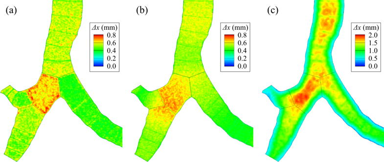
The CL-based geometric airway models proposed by Miyawaki et al. (2016) consist of straight-CL, curved-CL, and fitted-surface (FS) models, in which a branch is a cylinder, a curved pipe, and a pipe with irregular CL and cross-sections, respectively. In this study we compared the FS model to the CT-based model used by Miyawaki et al. (2012) in terms of air-flow field and aerosol distribution. In the CT-based model, a wall boundary was obtained from a CT-image, and inlet, outlet, and internal boundaries were defined manually. In contrast, the CL-based model is constructed in a way that anatomical information regarding branches are embedded and external and internal boundaries, surrounding each branch, can be easily defined (Figure 1). As described in detail below, these features of the CL-based model greatly facilitate pre- and post-processing of the input and output data of gas-flow and aerosol deposition simulations.

Figure 1.

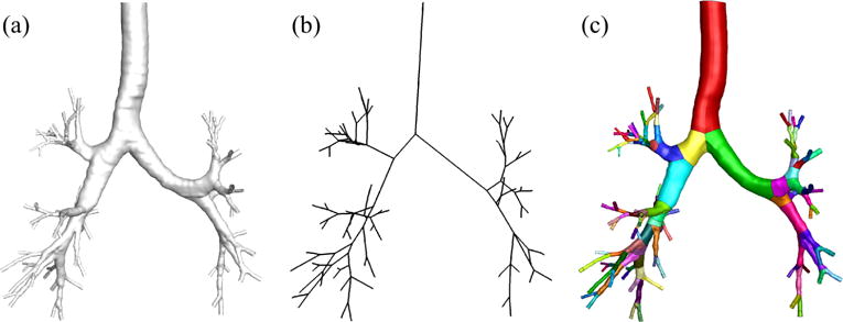
(a) The surface of computed tomography-based model, (b) skeleton, and (c) surface of fitted-surface model.

When constructing the geometric model, we extended the 1-D tree from the trachea to larynx using the average imaged tracheal diameter. From the fluid mechanical point of view, the normal narrowing within the glottal region plays a crucial role in creating turbulent laryngeal jet during inhalation (Dekker (1961), Lin et al. (2007), and Miyawaki et al. (2012)), but CT data usually do not include the region proximal to the trachea. Therefore, the geometry around the larynx needs to be modeled to replace missing extra-thoracic images. The geometry of larynx varies from subject to subject, so our goal is to devise a laryngeal model that can create a realistic level of turbulence in the trachea. We modeled the geometry of larynx using five parameters: location of the glottis L_g, (hydraulic) diameter at the glottis D_h,g, (hydraulic) diameter proximal to the glottis D_h,gu, length of the larynx proximal to the glottis l_gu, and length of the larynx peripheral to the glottis l_gl (Figure 2). We normalized the five parameters by the subject-specific hydraulic diameters of their trachea D_h,t, e.g., $L_g^{\ast }=L_g/D_{h,t}$, thus facilitating the application of the developed methodologies to future subjects.

Figure 2.

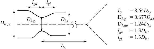
The definition and the values of the parameters to construct the geometric laryngeal model. The hydraulic diameter of the trachea D_h,t, the location of the glottis L_g, the (hydraulic) diameter at the glottis D_h,g, the (hydraulic) diameter proximal to the glottis D_h,gu, the length of upper part of the glottis l_gu, and the length of lower part of the glottis l_gl.

To empirically determine the five parameters, we used the data in the literature and the CT images of healthy subjects. We primarily used the data reported by Cheng et al. (1997) together with CT images of two healthy subjects. The University of Iowa Institutional Review Board and radiation safety committee approved the associated prior human studies and the use of these data for the current purposes. Cheng et al. (1997) did not report the inflation level, while the inflation levels for the CT images of the two healthy subjects were 90 percent vital capacity (“end inspiration”). In the previous imaging studies, the extra-thoracic airway was imaged during inhalation so as to assure that the glottis was fully open. Imaging of the lung itself was achieved with a linked spiral scan commencing after arrival at 90% vital capacity at which point the subject remained apneic (Lin et al. (2007), Choi et al. (2009), Yin et al. (2013)). There is no precise definition of the beginning of trachea, and CT imaging would not necessarily start from the beginning of trachea even if there was such a definition. The nearest benchmark that is included in most CT image data is carina occurring at the bifurcation of the right and left main stem bronchi. Thus, we empirically determined the distance between the glottis and the carina $L_g^{\ast }$. Since Cheng et al. (1997) did not report this distance, we obtained the distance from the data reported by Choi et al. (2009). We plotted the distribution of $D_h^{\ast }$ around the larynx to empirically determine $D_{h,g}^{\ast }$ and $D_{h,gu}^{\ast }$, and to empirically determine $l_{\mathit{gu}}^{\ast }$ and $l_{\mathit{gl}}^{\ast }$ by manually fitting the cubic Hermite spline curve (Fernandez et al., 2004). The normalized location of the glottis, $L_g^{\ast }(=L_g/D_{h,t})$, was 8.64 (± 0.58). The value in the parenthesis indicates the standard error. The normalized hydraulic diameters at the glottis and proximal to the glottis were 0.677 (± 0.054) and 1.24 (± 0.06), respectively. The optimal normalized lengths of the larynx proximal and peripheral to the glottis, $l_{\mathit{gu}}^{\ast }$ and $l_{\mathit{gl}}^{\ast }$, were both 1.3 (Figure 3)

Figure 3.

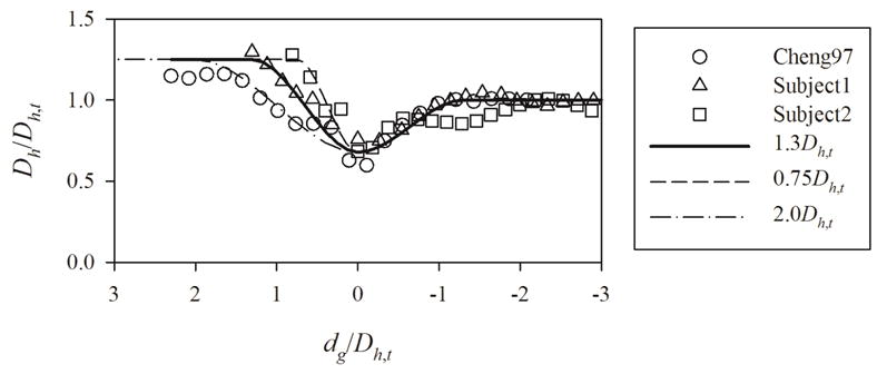
The geometric laryngeal model constructed using the geometries of Cheng et al. (1997) (Cheng97) and two healthy subjects (Subject1 and Subject2). The lengths of larynx proximal the glottis normalized by the (hydraulic) diameter of the trachea $l_{\mathit{gu}}^{\ast }$ for the model represented by solid, dashed, and dash-dotted curves are 1.3, 0.75, and 2.0, respectively. D_h,t, D_h, and d_g denote the hydraulic diameter of the trachea, hydraulic diameter of a cross-section in the larynx, and the distance from the glottis to the cross-section, positive in upward direction, respectively.

2.2. CFD mesh generation

We meshed the FS geometric model using Gmsh (Geuzaine and Remacle, 2009) and TetGen (Si, 2013) so that we can (a) partition the domain branch-by-branch, (b) automatically generate mesh, (c) generate mesh branch-by-branch, and (d) generate non-uniform mesh. Because the mesh is based on the 1-D tree, we can

• correlate simulation results with anatomical information regarding branches,

• use idealized 3-D airway geometry with arbitrary 1-D tree,

• systematically specify grid size, specify boundary conditions,

• reduce the data obtained from simulations branch-bybranch,

• generate volume mesh in parallel,

• easily identify errors while meshing volume, and

• generate non-uniform mesh in axial and radial directions.

To guarantee mesh consistency on the internal boundaries between neighboring branches, we first generated the surface mesh of the whole geometric model in serial, and then generated the volume mesh in parallel, preserving the surface mesh.

We computed the grid size using branch diameters and flow rates such that the grid size in every branch is similar to each other in terms of wall units. The image registration of two CT images can predict the flow rate in each branch (Yin et al., 2010). To compute the grid size in a cross-section of branch Δx_b, we used the following equation:

$$\mathrm{\Delta }{x}_b=\min \left(\mathrm{\Delta }{x}_t\sqrt{\frac{D_b^3}{r_{Q,b}{D}_t^3},}\frac{D_b}{6}\right)$$ (1)

where Δx_t is the grid size in the trachea, D_t is the trachea diameter, D_b is the branch diameter, and r_Q,b is the ratio of branch to trachea flow rate. Derivation of Equation 1 is presented in Appendix, and we determined Δx_t on the wall so that the grid size is comparable to the thickness of viscous sub-layer in the trachea, where flow is the most turbulent. The grid size Δx_b is not greater than D_b/6 to guarantee the accuracy of the flow field.

We generated non-uniform meshes in each branch by means of a background mesh. Volume grid size can be non-uniform in the axial direction of the lung-scale even if the size is uniform in each branch (uniform mesh), and the uniform mesh can be used for our CFD simulation since the surface grid size is consistent across the internal boundaries. However, the uniform mesh may yield inaccurate results, and the volume grid size should be non-uniform at the branch-scale such that size varies smoothly in the axial direction across internal boundaries (non-uniform mesh). In addition, depending on the flow rate, volume grid size near the lumen centers can be larger than the size near the walls to reduce computational time. The algorithm to generate non-uniform mesh in both axial and radial directions is as follows:

• Construct surface geometry using the FS method (Miyawaki et al., 2016) (Figure 4(a))

• Generate uniform background mesh by providing surface geometry and branch grid sizes to Gmsh (Figure 4(b))

• Compute non-uniform grid size distribution in each branch using diameter and flow rate (Figure 4(c))

• Generate non-uniform surface mesh by providing surface geometry and non-uniform grid size distribution to Gmsh (Figure 4(d))

• Generate non-uniform volume mesh by providing surface geometry, non-uniform grid size distribution, and non-uniform surface mesh to TetGen (Figure 4(d))

Figure 4.

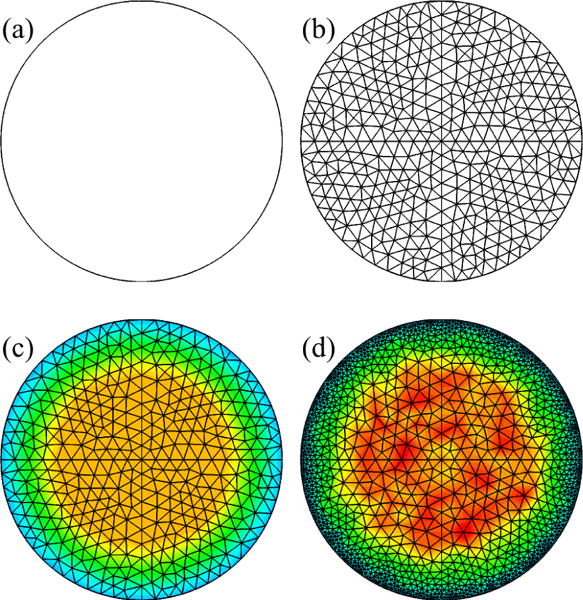
Generation of non-uniform mesh using background mesh: (a) geometry, (b) background mesh, (c) grid-size distribution, and (d) non-uniform mesh.

Again, the surface mesh was generated in serial, while the volume mesh was generated in parallel, preserving the surface mesh.

We obtained the grid-size distribution in the radial direction using a geometric progression such that the grid size increases from the wall to the free stream by a factor of a common ratio, until the grid size reaches the size in the free stream:

$$\mathrm{\Delta }{x}_d=\min (\mathrm{\Delta }{x}_w{r}_x^{n-1},\mathrm{\Delta }{x}_f)$$ (2)

$$n=\max \left\{\frac{\ln \left[1-\frac{(1-r_x)d}{\mathrm{\Delta }{x}_w}\right]}{\ln r_x},1\right\}$$ (3)

where Δx_d is the grid size at a point where distance from the wall is d, Δ_w is the grid size at the first node from the wall, Δx_f is the grid size in the free stream, r_x is the common ratio, 1.3 in this study. Note that grid size on the wall is Δx_w as well, and n is not necessarily an integer number, depending on d. We used three Δx_f, (1.0, 1.5, 2.8)Δx_w in the trachea or (2.3, 3.3, 6.3)×10⁻² D_t, to find the optimal value in terms of accuracy and computational cost, although Δx_f could be the same as Δx_w due to relatively small Reynolds number (Re), ~ 1000 – 2000, in the trachea (Re_t).

After generating the mesh, we extracted the boundary and volume meshes for each branch to specify the boundary conditions in the gas-flow simulation and to post-process the results from the aerosol simulation. The CFD mesh for each branch consists of top, bottom, and side boundary meshes and one volume mesh. The top and bottom are internal boundaries in most of branches, but they can be external boundaries in beginning and ending branches. It is straightforward to specify the boundary conditions in the gas-flow simulation and to count the number of aerosols passing through the internal or external boundaries for each segment in the aerosol simulation, because the boundary and volume meshes are consistent with the branches in 1-D tree (Figure 1).

2.3. Gas-flow simulation

To simulate air flow in the human airway model, we used the large eddy simulation (LES) model validated by Lin et al. (2005) and Choi et al. (2009). For comparison purposes, the breathing pattern was the same as that used by Miyawaki et al. (2012), i.e., steady inspiratory flow rate of 342 mL/s (~ 20 L/min) for a time period of 2.16 sec. The Reynolds number at the trachea Re_t was about 1,300. We imposed a turbulent flow above the glottis as explained later, the laminar parabolic flow at the end of the model as in Yin et al. (2010), and no-slip boundary condition on the airway wall.

We fed a homogeneous isotropic turbulent flow proximal to the glottis to use the laryngeal geometric model for CT-images without the extra-thoracic region. The flow becomes turbulent in the oral cavity and the time-averaged velocity profile is nearly uniform over the cross-section proximal the glottis when the parabolic laminar flow is fed at the mouth piece (Choi et al., 2009). It is also known that the turbulence of the flow upstream of a narrowing greatly affects the characteristics of the jet downstream of the narrowing. Therefore, a turbulent flow with a uniform time-averaged velocity profile needs to be fed proximal to the glottis if the geometric model does not include the extra-thoracic region. The geometry of the larynx was unknown and approximated, so using isotropic turbulent flow is the best approximation.

To reproduce the homogeneous isotropic turbulent flow proximal the glottis, we used the synthetic eddy method (SEM) proposed by Jarrin et al. (2009). The SEM is one of the simplest methods to reproduce synthetic turbulent flows that have correlation in time and space. The SEM does not require a 3-D turbulent flow field a priori, but instead reproduces synthetic turbulence as simulations go at the inlet surface. The only input parameters for the SEM are the length scale and Reynolds stress tensor of the turbulent flow. The Reynolds stress tensor of a homogeneous isotropic turbulent flow can be built using only turbulent intensity. Therefore, the SEM requires only the length scale and intensity of homogeneous isotropic turbulence. We obtained the two parameters as functions of Re_t from the results of simulations performed by Miyawaki et al. (2012) (Figure 5):

$$L_v/D_t=\{\begin{array}{ll}2.20\hfill & (R{e}_t\le 460)\hfill \\ 5300\times R{e}_t^{-1.27}\hfill & (460\le R{e}_t\le 2800)\hfill \\ 0.222\hfill & (2800\le R{e}_t)\hfill \end{array}$$ (4)

$$v_{\mathit{rms}}/U_t=\{\begin{array}{ll}0\hfill & (R{e}_t\le 202)\hfill \\ 0.0411\times \text{ln}(R{e}_t)-0.218\hfill & (202\le R{e}_t\le 2800)\hfill \\ 0.108\hfill & (2800\le R{e}_t)\hfill \end{array}$$ (5)

where L_v is the largest eddy size, v_rms is the space-averaged velocity root-mean-square in a cross-section proximal to the glottis, the parameters were normalized by the trachea diameter (D_t), 18.8 mm, and the bulk velocity in the trachea (U_t), 1.24 m/s, and the correlation coefficients of linear regression for L_v/D_t and v_rms/U_t were −0.98 and 0.97, respectively.

Figure 5.

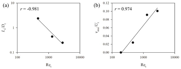
Distributions of (a) largest eddy size (L_v) and (b) space-averaged velocity root-mean-square (v_rms) in a cross-section at epiglottis level for the three Reynolds numbers based on the trachea diameter (Re_t) 460, 1300, and 2800, normalized by the trachea diameter (D_t), 18.8 mm, and bulk velocity in the trachea (U_t), 1.24 m/s, respectively. “r” denotes the correlation coefficient of linear regression. See Equations 4 and 5 for the equations of the regression curves in (a) and (b), respectively.

2.4. Aerosol simulation

To simulate the aerosol transport in the numerical airway model, we used the Lagrangian tracking algorithm validated by Miyawaki et al. (2012). Miyawaki et al. (2012) found the aerosols are well distributed over the cross-section proximal to the glottis when air was used as the carrier gas. According to Grgic et al. (2004), about 50% of 20-μm particles would pass oral cavity given the geometry and flow rate in Miyawaki et al. (2012) and this study. In this study, 88, 87, 82, 50, and 3% of 1.0, 2.5, 5.0, 10, and 20-μm particles exited the computational domain, i.e., large airways, respectively. As a result, 20-μm particles deposited in the large airways most, and thus we used them in our analysis to minimize the influence of uncertainty in our model. We considered the oral deposition using the empirical curve proposed by Grgic et al. (2004) when determining the size of the aerosols that deposit most in the central branches. In this study, we released 100,000 of 20-μm aerosols uniformly over the cross-section proximal the glottis so that at least 10 particles enter more than 95% of branches. We updated the flow field every 0.006 sec and released the aerosols 8 times with interval of 0.048 sec to account for the unsteady nature of air flow as in Miyawaki et al. (2012). To evaluate the performance of the FS model, we computed deposition efficiency (DE) for each branch:

$$DE=N/M$$ (6)

where M and N are the numbers of aerosols entered and deposited in the branch. We computed N using the side boundary mesh, and computed M by adding N of own and descendant branches using skeleton connectivity.

3. Results

3.1. Aerosol deposition

To evaluate the performance of the proposed method in predicting aerosol deposition, we compared the DE predicted by the current method that sets Δx_f = Δx_w with that predicted by the CT-based model used by Miyawaki et al. (2012). To compute DE in the CT-based model in the way that is consistent with the FS model used by the proposed method, we first repeated the aerosol simulations performed by Miyawaki et al. (2012) using 220,000, instead of 10,000, particles so approximately 100,000 particles enter the trachea. Second, we partitioned the surface of the CT-based model into branches using the surface of the FS model. The correlation coefficient, slope, and intercept of linear regression between the DE in branches of the FS model and that in the CT-based model were 0.93, 0.95, and 0.0037, respectively (Figure 6). There exist some outliers in Figure 6 for 20-μm particles. To examine whether these outliers are branch-specific, we also computed the correlations for 10-μm particles (not shown). The results showed that the outliers for 20-μm particles are not necessarily those for 10-μm particles.

Figure 6.

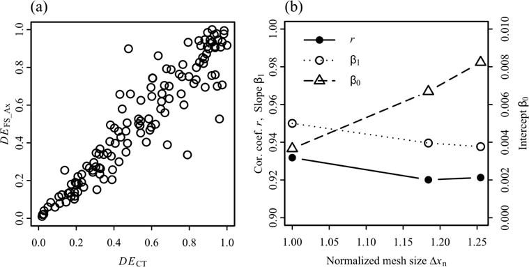
The correlations between the deposition efficiencies (DE) of 20-μm aerosols in computed tomography (CT)-based model and fitted-surface (FS) models: (a) the CT-based model vs. the FS model with non-uniform mesh in axial direction, (b) correlation coefficients, slopes, and intercepts of linear regression lines for the CT-based model vs. the FS models. The number of elements (N_e,n) and normalized average grid size (Δx_n) in the FS models with non-uniform mesh in axial direction, non-uniform fine mesh in axial and radial direction, and non-uniform coarse mesh in axial and radial direction are (N_e,n, Δx_n) = (1.00, 1.00), (0.60, 1.18), and (0.51, 1.25), respectively, where Δx_n = (1/N_e,n)^1/3.

3.2. Laryngeal model

To examine the performance of the approximate laryngeal model, we compared the turbulent kinetic energy (TKE) distribution in the trachea predicted with the CT-based and laryngeal (Δx_f = Δx_w) models (Figure 7). In the CT-based model, we imposed laminar flow at the mouthpiece, while we used SEM to feed turbulent flow proximal to the glottis in the laryngeal model. The laryngeal jet was not parallel to the airway direction in the CT-based model, and TKE was amplified in the shear layer around the jet (Figure 7(a)). The jet was parallel to the airway direction in the approximate model, and the approximate model captured the amplification of TKE in the shear layer around the laryngeal jet (Figure 7(b)).

Figure 7.

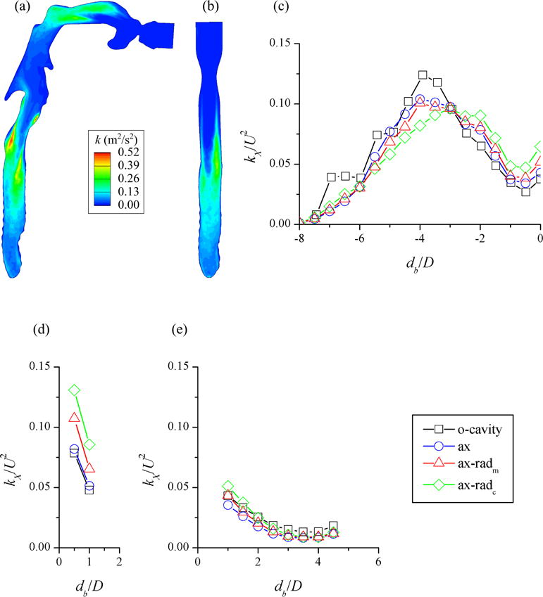
The turbulent kinetic energy (TKE, k) distributions in the plane through the center of the trachea predicted with the (a) CT-based model with oral cavity (“o-cavity”) and (b) fitted-surface model with non-uniform CFD mesh in axial direction (“ax”). The distributions of cross-sectional averaged TKE (k_X) normalized by the bulk velocity squared (U²) in the (c) trachea, (d) RMB, and (e) LMB for “o-cavity” (fine mesh), “ax” (fine mesh), non-uniform medium mesh in axial and radial directions (“ax-rad_m”), and non-uniform coarse mesh (“ax-rad_c”). d_b and D are distance from the first bifurcation and branch hydraulic diameter, respectively.

Since cross-sections in the trachea were not axisymmetric, we compared the cross-sectional averaged TKE (k_X) distributions along the trachea of the two models (“o-cavity” and “ax” in Figure 7(c)). The distance between the peaks of k_X distributions was shorter than a half trachea hydraulic diameter, while the simulation with the laryngeal model underestimated highest cross-sectional averaged TKE by 16%. When we fed laminar flow proximal to the glottis in the approximate model (not shown), TKE was negligible compared to the CT-based model. The average relative differences in k_X/U² along the right main bronchus (RMB) and the left main bronchus (LMB) were 6 and 33%, respectively (Figures 7(d)(e)). Note k_X/U² in the LMB (~ 0.02 on average) was about a third of that in the RMB. Overall, k_X/U² in the trachea, RMB, and LMB for the two models agreed reasonably well.

3.3. Non-uniform mesh

To find the optimal grid size in the free stream, Δx_f, we compared the aerosol deposition in the central airway and TKE distribution along the trachea predicted with the FS models with three different Δx_f: fine, medium, and coarse. The numbers of elements (N_e) and average grid sizes (Δx) for the mesh Δx_f = (1.0, 1.5, 2.8)Δx_w normalized by the respective values for the fine mesh were N_e,n = (1.00, 0.60, 0.51) and Δx_n = (1.00, 1.18, 1.25), respectively, where N_e for the fine mesh was 18.5 million and Δx_n = (1/N_e,n)^1/3 (Figure 8). In the non-uniform mesh in axial direction (Figure 9(b)), grid size varied more continuously across internal boundaries between neighboring branches than in uniform mesh (Figure 9(a)). In addition, mesh is refined near the wall in the non-uniform mesh in axial and radial directions (Figure 9(c)).

Figure 8.

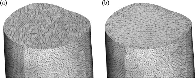
The (a) fine (“ax” in Figure 7) and (b) coarse (“ax-rad_c” in Figure 7) meshes at the proximal end of the trachea.

Figure 9.

The distributions of grid size (Δx) around the first bifurcation: (a) uniform mesh in each branch, (b) non-uniform mesh in axial direction (“ax” in Figure 7), and (c) non-uniform mesh in axial and radial directions (“ax-rad_c” in Figure 7).

Similar to the fine mesh, we computed the correlation coefficient, slope, and intercept of linear regression between deposition efficiencies predicted with the other two meshes and the CT-based model (Figure 6(b)). The correlation coefficients for medium and coarse meshes were larger than 0.92, slopes were both 0.94, and intercepts were less than 0.009. In addition, we compared the TKE distributions along the trachea of the other two meshes and the CT-based model. The medium and coarse meshes underestimated the peak TKE by 19% and 22%, respectively. The distance between the location of peak TKE in the medium mesh and that in the CT-based model was less than a half hydraulic diameter of the trachea; while the location of peak TKE in the coarse mesh was one hydraulic diameter downstream of that in the CT-based model. The average relative differences in k_X/U² along the RMB were 73 and 37% for the coarse and medium mesh, respectively, while those along the LMB were 21 and 24% (Figures 7(d)(e)). Again, k_X/U² in the LMB was small (~ 0.02 on average).

4. Discussion

4.1. Aerosol deposition

To evaluate the ability of the FS model in predicting aerosol deposition, we compared the depositions of 20 μm-aerosols in the FS model developed by Miyawaki et al. (2016) and the CT-based model used by Miyawaki et al. (2012). The deposition efficiencies (DEs) in the branches of the FS model were strongly correlated with those in the CT-based model. In addition, the slope of the linear regression between the DEs in the FS and CT-based models deviated from one by 0.05, and the intercept of the correlation was less than 0.01. Based on the comparison between the numerical simulations by Miyawaki et al. (2012) and the experiments by Grgic et al. (2004), the uncertainty in the prediction of deposition efficiency is about 0.07 at low Stk·Re^0.37. Therefore, as expected, the quality of the automatically generated CFD mesh based on the FS model is high enough to predict aerosol deposition. The FS model may be used especially for studies that involve multiple subjects because this method requires much less time to pre- and post-process data compared to the CT-based models constructed manually.

4.2. Laryngeal model

To construct an idealized laryngeal model, we empirically determined the dimensions of larynx. The fitted curve represented the distributions of $D_h^{\ast }$ in the geometries of three subjects reasonably well. According to Choi and Wroblewski (1998), the ratio of cross-sectional area at the glottis to trachea is 0.40 at mid-inspiration, i.e., $D_{h,g}^{\ast }$ is 0.63 with the assumption of circular cross-section. The $D_{h,g}^{\ast }$ found in this study is consistent with the published value for mid-inspiration.

We used the empirically determined parameters to model laryngeal geometry and SEM to reproduce turbulent laryngeal jet. The approximate laryngeal model captured overall distribution of TKE in the trachea, and the highest TKE values predicted by the laryngeal and CT-based models were of the same order of magnitude. We concluded that the laryngeal model reproduced a realistic level of turbulence given that (a) we defined the geometry of the larynx with only five parameters, (b) we only specified the largest eddy size and turbulent intensity as input to generate isotropic turbulent flow proximal the glottis, and (c) we did not optimize the parameters specifically for this subject.

If the airway geometry proximal to the trachea is unknown, the turbulent flow generated with this laryngeal model would be accurate enough. If the applications are concerned with particle depositions in the central airways, subject-specific models in the extra thoracic regions may not be important. On the other hand, if the applications are concerned with flow structures and particle deposition close to the glottis, subject-specific models in that region are certainly important.

4.3. Non-uniform mesh

In addition to a non-uniform mesh in the axial direction, we used two more meshes with non-uniform grid-size distributions in the radial direction to find the optimal grid size away from the wall in terms of computational speed and accuracy. The aerosol depositions assessed via the medium and coarse meshes, whose free stream grid sizes were 18% and 25% larger than the size in fine mesh, respectively, were as accurate as that observed using the fine mesh. The TKE distribution in the trachea of the medium mesh was also as accurate as the fine mesh, while the location of the peak TKE in the coarse mesh was down stream of the other meshes by one hydraulic diameter of the trachea. The computational cost for the medium mesh was 51% of that for the fine mesh. Therefore, one may save computational time by factor of two without losing accuracy by using the medium mesh, whose free stream grid size is 3.3% of the diameter in the trachea, for the same breathing pattern.

We calculated the grid size in each branch relative to the trachea using the branch diameter and flow rate relative to the trachea (Equation 1). This method can be applied to subject-specific models as well as representative models. In this study, we obtained subject-specific branch diameter and flow rate by CT image segmentation and registration. If such data are not available, one could instead use, e.g., the model by Horsfield et al. (1971) based on a healthy subject, to obtain the branch diameter and flow rate.

4.4. Advantages

The CL-based model is basically an extension of 1-D tree to 3-D geometry, and the major advantages of these models are related to this modeling philosophy. Since these models are extended from 1-D tree, one sub-domain corresponds to one branch. This is a very important feature of numerical models for the following nine reasons. First, we can create the geometry via generated or idealized skeletons using the straight-CL model. Second, we can create the geometry with idealized diameters using the curved-CL model. Third, we can create the geometry that includes CT-resolved and CT-unresolved branches combining the FS and curved-CL models. Fourth, we can generate CFD mesh for branches in parallel. Fifth, we can easily impose boundary conditions using, e.g., flow rate and diameter even for a large number of branches. Sixth, we can map the surface and volume elements in the CT-based model to branches using FS model. Seventh, we can easily compute branch-averaged quantity during/after gas-flow simulations. Eighth, we can easily count the number of aerosol particles entering and depositing along branches during/after aerosol simulations. Because of the seventh and eighth features, we can investigate the correlation between the quantities for branches with the geometric properties of the branches, e.g., diameter, length, curvature, branching angle, and gravity angle. Ninth, we can investigate multiple subjects more easily than has previously been possible when using more traditional, manual methods. For example, the method proposed by Marchandise et al. (2013) does not have the first three features, despite the high quality of their CFD mesh for CT-resolved branches. The elements in their CFD mesh can be mapped to branches using the FS model for post-processing.

4.5. Limitations

In this study we did not consider the other functions of extra-thoracic region in drug delivery, but they could be included depending on the purpose of the simulations. An important function is the filtering of aerosols due to oral deposition. This can be implemented using the similarity curve based on the experiments conducted by Grgic et al. (2004) (Grgic’s curve). The seven parameters, five for geometry and two for gas-flow, for the approximate laryngeal model could be improved by studying more subjects. It would be ideal to find an empirical formula for those parameters based on the clinical characteristics of the subjects, the subject-specific breathing patterns, and the geometry of trachea such that the parameters can be determined even if CT images do not include the extra-thoracic region. In addition, the differences in inhalation pattern and mouthpiece geometry should be incorporated in the future by investigating the correlation between the particle distributions at the mouthpiece and proximal to the glottal constriction under different inhalation patterns.

Since grid size distribution can be arbitrary using the proposed method, grid size distribution can be obtained using the results from preliminary simulations to determine if a higher quality mesh is needed. In this study, we used only tetrahedral elements due to relatively low Re and complex geometry around branching points. In the future, prism elements could be used near airway wall to efficiently resolve boundary layer for breathing patterns with higher Re.

5. Conclusions

The aerosol deposition in the central airways and turbulence in the trachea predicted by the proposed model agreed well with the prediction by a traditional CT-based model. This implies that the semi-automatically constructed geometric model, including the idealized laryngeal model, can be used for the CFD-based simulations of aerosol depositions in individual human lungs with a reasonable level of accuracy. The new method would allow researchers to simulate aerosol depositions in multiple subjects and study pulmonary aerosol delivery to the human lungs, taking inter-subject variabilities into consideration.

Highlights.

• We developed an idealized laryngeal model to replace missing extrathoracic images.

• The new method automatically meshed human airway geometries.

• The new method accurately predicted the aerosol depositions in the central airways.

• The laryngeal model generated a realistic level of turbulence in the trachea.

• The new method is suited for analysis of aerosol distribution in multiple subjects.

Appendix A. Derivation of local grid size

In a laminar fully-developed pipe (Poiseuille) flow the wall shear stress τ_w is

$${\tau }_w=\frac{8\mu U_b}{D_b}$$ (A.1)

where μ is the dynamic viscosity of the fluid, U_b is the branch bulk velocity, and D_b is the branch diameter. Equation A.1 can be expressed using the ratio of branch to the trachea flow rate r_Q,b as

$${\tau }_w=8\mu \frac{4Q_t{r}_{Q,b}}{\pi D_b^2}\frac{1}{D_b}=c\frac{r_{Q,b}}{D_b^3}$$ (A.2)

where Q_t is the flow rate in the trachea and c is a constant for any branch. Equation A.2 is used to get the friction velocity u* as

$$u^{\ast }=\sqrt{{\tau }_w/\rho }=c\sqrt{r_{Q,b}/D_b^3}$$ (A.3)

and the grid size in wall unit y⁺ as

$$y^{+}=\frac{u^{\ast }y}{v}=c\mathrm{\Delta }{x}_b\sqrt{\frac{r_{Q,b}}{D_b^3}}$$ (A.4)

where ρ is the density of the fluid and Δx_b is the branch grid size. When y⁺ is constant for any airway, the local grid size can be obtained using the trachea grid size Δx_t:

$$\mathrm{\Delta }{x}_b=\mathrm{\Delta }{x}_t\sqrt{\frac{D_b^3}{r_{Q,b}{D}_t^3}}$$ (A.5)

where the flow rate ratio for the trachea r_Q,t is 1.

References

- Bennett WD, Brown JS, Zeman KL, Hu SC, Scheuch G, Sommerer K. Targeting delivery of aerosols to different lung regions. Journal of aerosol medicine. 2002;15:179–188. doi: 10.1089/089426802320282301. [DOI] [PubMed] [Google Scholar]
- Cheng KH, Cheng YS, Yeh HC, Swift D. Measurements of airway dimensions and calculation of mass transfer characteristics of the human oral passage. Journal of Biomechanical Engineering. 1997;119:476. doi: 10.1115/1.2798296. [DOI] [PubMed] [Google Scholar]
- Choi J, Tawhai MH, Hoffman EA, Lin CL. On intra-and inter-subject variabilities of airflow in the human lungs. Physics of Fluids. 2009;21:101901. doi: 10.1063/1.3247170. [DOI] [PMC free article] [PubMed] [Google Scholar]
- Choi Y, Wroblewski D. Characteristics of glottis-induced turbulence in oscillatory flow: An empirical investigation. Journal of Biomechanical Engineering. 1998;120:217. doi: 10.1115/1.2798305. [DOI] [PubMed] [Google Scholar]
- Dekker E. Transition between laminar and turbulent flow in human trachea. Journal of applied physiology. 1961;16:1060–1064. doi: 10.1152/jappl.1961.16.6.1060. [DOI] [PubMed] [Google Scholar]
- van Ertbruggen C, Hirsch C, Paiva M. Anatomically based three-dimensional model of airways to simulate flow and particle transport using computational fluid dynamics. Journal of applied physiology. 2005;98:970–980. doi: 10.1152/japplphysiol.00795.2004. [DOI] [PubMed] [Google Scholar]
- Fernandez J, Mithraratne P, Thrupp S, Tawhai M, Hunter P. Anatomically based geometric modelling of the musculo-skeletal system and other organs. Biomechanics and Modeling in Mechanobiology. 2004;2:139–155. doi: 10.1007/s10237-003-0036-1. [DOI] [PubMed] [Google Scholar]
- Gemci T, Ponyavin V, Chen Y, Chen H, Collins R. Computational model of airflow in upper 17 generations of human respiratory tract. Journal of Biomechanics. 2008;41:2047–2054. doi: 10.1016/j.jbiomech.2007.12.019. [DOI] [PubMed] [Google Scholar]
- Geuzaine C, Remacle JF. Gmsh: A 3-D finite element mesh generator with built-in pre-and post-processing facilities. International Journal for Numerical Methods in Engineering. 2009;79:1309–1331. doi: 10.1002/nme.2579. [DOI] [Google Scholar]
- Grgic B, Finlay WH, Burnell PKP, Heenan AF. In vitro intersubject and intrasubject deposition measurements in realistic mouth-throat geometries. Journal of Aerosol Science. 2004;35:1025–1040. [Google Scholar]
- Horsfield K, Dart G, Olson DE, Filley GF, Cumming G. Models of the human bronchial tree. Journal of Applied Physiology. 1971;31:207–217. doi: 10.1152/jappl.1971.31.2.207. [DOI] [PubMed] [Google Scholar]
- Jarrin N, Prosser R, Uribe JC, Benhamadouche S, Laurence D. Reconstruction of turbulent fluctuations for hybrid rans/les simulations using a synthetic-eddy method. International Journal of Heat and Fluid Flow. 2009;30:435–442. doi: 10.1016/j.ijheatfluidflow.2009.02.016. [DOI] [Google Scholar]
- Lin CL, Lee H, Lee T, Weber LJ. A level set characteristic galerkin finite element method for free surface flows. International Journal for Numerical Methods in Fluids. 2005;49:521–547. [Google Scholar]
- Lin CL, Tawhai MH, McLennan G, Hoffman EA. Characteristics of the turbulent laryngeal jet and its effect on airflow in the human intra-thoracic airways. Respiratory physiology & neurobiology. 2007;157:295–309. doi: 10.1016/j.resp.2007.02.006. [DOI] [PMC free article] [PubMed] [Google Scholar]
- Longest PW, Tian G, Walenga RL, Hindle M. Comparing mdi and dpi aerosol deposition using in vitro experiments and a new stochastic individual path (sip) model of the conducting airways. Pharmaceutical research. 2012;29:1670–1688. doi: 10.1007/s11095-012-0691-y. received: 21 October 2011/Accepted: 19 January 2012/Published online: 31 January 2012. [DOI] [PubMed] [Google Scholar]
- Marchandise E, Geuzaine C, Remacle J. Cardiovascular and lung mesh generation based on centerlines. International journal for numerical methods in biomedical engineering. 2013;29:655–682. doi: 10.1002/cnm.2549. [DOI] [PubMed] [Google Scholar]
- Miyawaki S, Tawhai MH, Hoffman EA, Lin CL. Effect of carrier gas properties on aerosol distribution in a CT-based human airway numerical model. Annals of biomedical engineering. 2012;40:1495–1507. doi: 10.1007/s10439-011-0503-2. [DOI] [PMC free article] [PubMed] [Google Scholar]
- Miyawaki S, Tawhai MH, Hoffman EA, Wenzel SE, Lin CL. Automatic construction of subject-specific human airway geometry including trifurcations based on a ct-segmented airway skeleton and surface. Biomechanics and Modeling in Mechanobiology. 2016:1–14. doi: 10.1007/s10237-016-0838-6. [DOI] [PMC free article] [PubMed] [Google Scholar]
- Si H. TetGen: A Quality Tetrahedral Mesh Generator and 3D Delaunay Triangulator. (1.5) 2013 [Google Scholar]
- Tawhai MH, Hoffman EA, Lin CL. The lung physiome: merging imaging-based measures with predictive computational models. Wiley Interdisciplinary Reviews: Systems Biology and Medicine. 2009;1:61–72. doi: 10.1002/wsbm.17. [DOI] [PMC free article] [PubMed] [Google Scholar]
- Tian G, Longest P, Su G, Walenga RL, Hindle M. Development of a stochastic individual path (SIP) model for predicting the tracheobronchial deposition of pharmaceutical aerosols: Effects of transient inhalation and sampling the airways. Journal of Aerosol Science. 2011;42:781–799. doi: 10.1016/j.jaerosci.2011.07.005. [DOI] [Google Scholar]
- Walters D, Burgreen G, Lavallee D, Thompson D, Hester R. Efficient, physiologically realistic lung airflow simulations. Biomedical Engineering, IEEE Transactions on. 2011;58:3016–3019. doi: 10.1109/TBME.2011.2161868. [DOI] [PubMed] [Google Scholar]
- Yin Y, Choi J, Hoffman EA, Tawhai MH, Lin CL. Simulation of pulmonary air flow with a subject-specific boundary condition. Journal of Biomechanics. 2010;43:2159–2163. doi: 10.1016/j.jbiomech.2010.03.048. [DOI] [PMC free article] [PubMed] [Google Scholar]
- Yin Y, Choi J, Hoffman EA, Tawhai MH, Lin CL. A multiscale MDCT image-based breathing lung model with time-varying regional ventilation. Journal of Computational Physics. 2013;244:168–192. doi: 10.1016/j.jcp.2012.12.007. [DOI] [PMC free article] [PubMed] [Google Scholar]