Accelerating physical simulations of proteins by leveraging external knowledge

Abstract

It is challenging to compute structure-function relationships of proteins using molecular physics. The problem arises from the exponential scaling of the computational searching and sampling of large conformational spaces. This scaling challenge is not met by today’s methods, such as Monte Carlo, simulated annealing, genetic algorithms, or molecular dynamics (MD) or its variants such as replica exchange. Such methods of searching for optimal states on complex probabalistic landscapes are referred to more broadly as Explore-and-Exploit (EE), including in contexts such as computational learning, games, industrial planning and modeling military strategies. Here we describe a Bayesian method, called MELD, that ‘melds’ together explore-and-exploit approaches with externally added information that can be vague, combinatoric, noisy, intuitive, heuristic, or from experimental data. MELD is shown to accelerate physical MD simulations when using experimental data to determine protein structures; for predicting protein structures by using heuristic directives; and when predicting binding affinities of proteins from limited information about the binding site. Such Guided Explore-and-Exploit approaches might also be useful beyond proteins and beyond molecular science.

Introduction: Global optima of complex landscapes can be found by explore-and-exploit methods

A challenge of computational modeling is how to search complex high-dimensional probability distributions efficiently, to find the states that are at the global maxima of highest probability. This problem is common across broad areas of statistical inference, industrial planning and optimization, science and technology research policy, ensemble weather forecasting^1,2, military strategies, biological evolution by mutation and natural selection, animal strategies of foraging for food, and in playing games such as chess and Go^3,4.

A major area of application is in the Computational Physical Modeling of Molecules (CPMM). CPMM is widely applied toward understanding molecular conformations, reaction mechanisms, adsorption and self assembly; to estimate the partitioning or transfer of molecules from one medium to another; and to compute the folding and binding properties of biomolecules such as proteins. Such modeling entails extensive conformational searching on very high-dimensional and rugged energy landscapes to seek the states having low free energies. States of low free energy are important because they dominate in nature, and in experiments, because they are the states of highest population. Various computational methods are used for searching (seeking particular states) and sampling (collecting sufficient statistics about those states to estimate populations), including Monte Carlo (MC)^5,6, Molecular Dynamics (MD)⁷, Replica Exchange⁸, Hamiltonian Exchange⁹, umbrella sampling¹⁰, steered Molecular Dynamics¹¹, metadynamics¹², simulated annealing¹³, and genetic algorithms¹⁴.

Search-and-sample methods can be described more broadly under the general term of Explore-and-Exploit^15–17. Explore refers to the parts of a search and sampling process that are relatively undirected forays into unexplored territory. Exploit refers to the parts of the search and sampling process that are relatively directed towards locally promising goals. Interestingly, humans appear to make decisions this way; there are different brain regions for explore vs. exploit as a neural mechanism for action selection¹⁸. A paradigmatic illustrative model in this area is the multi-armed bandit problem¹⁹, in which there are different slot machines, each having different probabilities of payoffs when a lever is pulled. Some machines pay a lot, but you do not know which. If some particular machine is paying off, you continue pulling that lever, but at the opportunity cost of possibly missing out on a machine having a bigger payoff. Exploitation is when you continue to pull a lever you already know is paying off. Exploring is when you pulling a new lever that you haven’t tried before, in the hopes of an even bigger payoff. The best strategies are known to begin with full exploration, then evolve towards more exploitation, but never to ‘full’ exploitation^20,21. Successful searching and sampling usually results from many alternating steps of exploring and exploiting. In attempting to fold a protein using this strategy, the computer exploits when searching downhill on local minima on free-energy landscapes, and explores when it traverses uphill or sideways on the landscape seeking deeper – possibly global – minima (see Figure 1).

Figure 1.

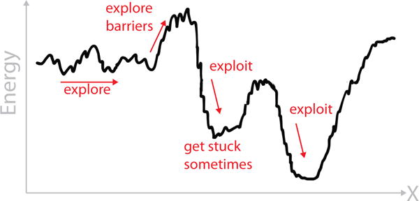
Explore-and-exploit is a general strategy for seeking a global optimum of an objective function (in this case, a free-energy minimum), on a landscape that is usually bumpy and high dimensional.

Here, we review a computational strategy, called MELD, that uses external knowledge, in guided exploring and exploiting, to accelerate goal finding. We illustrate it by application to three problems of protein modeling. MELD ‘melds’ together knowledge or heuristics or insights of some kind, with Molecular Dynamics forcefield simulations.

Searching and sampling is a challenge in computational protein modeling

Computer modeling is a major route for understanding the actions of the proteins, and for discovering new drugs. Modeling is challenging because of a protein’s several thousands of atoms and bonds, which are free to arrange in combinatorially many ways. And, a protein’s space of viable conformations is complex. Its free-energy surface is rugged and high-dimensional²² because the chain is a physical object that cannot pass through itself. A protein is a linear chain of 50 – 1000 amino acids, strung together like beads on a necklace. Each amino acid is composed of tens of atoms. Like a string in space, a protein molecule can adopt different possible conformations. Each protein conformation can be represented by a coordinate vector of its component atoms²³. The protein has many different atom types, and different atoms interact differently. A protein has a conformational energy^7,24 that is a function of its coordinate vector. Proteins are subject to the laws of thermodynamics, so the stable states of proteins are those conformations having globally minimal free energies. To find the structures that have the highest populations in nature, we seek the states of lowest free energy in computational models. And, populations are the essential starting point for understanding protein motions, binding, folding and biological actions.

A common way to simulate the physical properties of proteins is to use long unbiased MD simulations at an atomistic level of representation. In 1998, Duan and Kollman collected the first microsecond-long trajectories of the folding of the villin headpiece, among the smallest known folded proteins²⁵. The Duan-Kollman milestone paper appears to have been a key motivation for IBM’s development, very soon thereafter, of its Blue Gene computer³. Improvements in forcefields^26–33 and computer architecture^34,35 in the last 20 years have increased the accuracy and reduced the time needed to fold small proteins^36–42. The most recent advances in simulating larger and more interesting proteins comes from GPUs³⁷ and from a special-purpose supercomputer, called Anton, developed by DE Shaw Research^42,43. Despite these advances, physical simulations of folding, for example, are still limited to only the very smallest proteins and smallest motions and actions (see Box 1). Below, we describe an acceleration method that combines loose guidance based on some knowledge of the target objective, with explore-and-exploit searching-and-sampling methods.

Box 1. Why do physical modeling rather than knowledge-based modeling?

There have been two main computational approaches to harnessing experimental data in modeling protein structures. First, in an approach called Integrative Structural Biology, multiple sources of data are brought together, some noisy and ambiguous, with inferences about known protein structures, to make useful predictions of protein structures^44,45. In homology modeling, you draw inferences about the structure of your target protein by using knowledge of a template protein, which is a different protein that has known sequence and structure that is assumed to resemble your target molecule. This approach draws from a knowledgebase such as the Protein DataBank (PDB)^46,47. Such bioinformatic modeling is most useful when there are good templates in a knowledgebase^48,49 and when you seek a single optimal structure, rather than an ensemble or distribution of structures. One goo,,,,,,,d strategy has been to extract information from the PDB, either local (e.g. fragments) or global, to guide the search, and in so doing sample conformational space more efficiently and with correct “local free energies”^50–52. Even though this method entails exploration (via Monte Carlo or other sampling tools), it does not fully satisfy detailed balance.

The second approach, of interest here, is to use physics-based models of the energies (a forcefield), and to do explore-and-exploit simulations that obey detailed balance; this produces ensembles of states that are populated in accordance with the principles of statistical mechanics. Physics-based methods have the advantage of going beyond just structural information, to include energies, and therefore to predict populations, free energies, binding affinities, dynamics and mechanisms. Today’s disadvantages of physics-based approaches are that they are computationally slow – it has traditionally been relegated to sampling around native states^53–56 or refining structures derived from bioinformatics methods^49,57. Furthermore, these methods are only able to harness external information that is specific, accurate and unambiguous.

Physics-based methods are of growing importance thanks to recent advances in computers, forcefields and sampling methods. (1) While past simulations have been able to postdict known protein structures^{24,25,36–43,58–65}, more recent modeling is now fast enough to be predictive in blind tests^66,67. (2) Physical simulations are providing the atom-by-atom, picosecond by picosecond narratives for how we understand biological mechanisms^68–70) (3) forcefields continue to improve^71,72, and are even now applicable outside of protein modeling to other foldameric materials, where bioinformatics is not an option⁷³.

MELD: a method of ‘Loosely Guided’ Explore-and-Exploit

A general problem with computational exploring-and-exploiting is its inefficiency. Exploring large spaces can be slow. The need for searching grows exponentially with the number of degrees of freedom. In principle, if something is known about the target objective – even vaguely, it could accelerate the search to find the global optimum. In typical explore-exploit processes, the search process ‘doesn’t know what it’s looking for’. Physical simulations of biomolecules seek states of lowest free energy. But sometimes, we may have additional knowledge of where the target goal lies. For example, we might like to instruct an MD simulation of protein folding to ‘make a good hydrophobic core’, or ‘make good secondary structures’, or ‘make the folded state compact’ while it is simultaneously seeking the state of minimum free energy of a forcefield’s energy landscape. Furthermore, we may want to direct an MD simulation of a ligand binding to a protein to seek a binding site ‘in roughly the following vicinity’. Such instructions can capture our chemical intuition – resembling the way that computer algorithms in games such as chess or Go use heuristics and machine learning as a way of reproducing player intuition. But such instructions have been difficult to incorporate into MD simulations because they are too vague or combinatoric or fraught with misdirecting information.

An important example is combining experimental data with MD simulations to determine protein structures. At one extreme – when there is sufficient experimental data having plenty of good-quality restraints – MD may not be needed at all. Then, molecular structures can be determined directly from experiments alone. However, the opposite extreme is quite common – where experimental data is insufficient, either because it is too sparse, noisy or ambiguous. For an overview of data limitations from Nuclear Magnetic Resonance (NMR), Electron-Spin Resonance (ESR), probe-label methods or sequence-structure homologies see reference⁶⁴. Here are examples. NMR data has been used in modeling native states^74,75, dynamics of proteins⁷⁶ and ensembles of disordered proteins^77–79. Laio and Vendruscolo use this kind of data as objective seeking⁸⁰ by using chemical shifts from NMR as collective variables to explore the conformational landscape of protein G. Their approach is able to give free energies and populations because they use the data as a search method, not to restrain the energies. To make the sampling more efficient they use bias-exchange metadynamics (BE-META) where each replica has a collective variable. This approach converges much faster than regular metadynamics^12,81, wherein convergence is an exponential function of the number of collective variables. Another approach is based on metainference⁸², which combines elements of Bayesian inference and maximum entropy. Hummer and Kofinger have recently developed a Bayesian technique somewhat similar to MELD; it too treats the force-field as a prior distribution, and obtains the likelihood from experimental data⁷⁹. However, unlike in MELD, which seeks specific states corresponding to sub-collections of noisy information, their approach seeks distributions of disordered states of proteins where experimental information coincides with averages over the structural ensemble. A very exciting area of structure determination, for proteins or their complexes that are not currently accessible by other methods, is coming from X-ray Free-Electron Lasers (XFEL) and from Cryo-Electron Microscopy (CryoEM)^83–85.

We want a way to harness vague information in explore-and-exploit strategies. For biomolecule simulations, we want to harness vague information to speed up molecular dynamics simulations, without sacrificing the important capability that proper physical sampling methods have of preserving Boltzmann populations. Here, we describe a method called MELD that uses a Bayesian approach to find structures that both satisfy these insights and are compatible with the forcefield.

MELD uses Bayesian inference to choose favored options

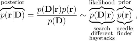
The problem of finding the native structure of a protein – the ‘one’ conformation at the global minimum of free energy – is like seeking the proverbial needle in a haystack. MELD does this using a Bayesian approach to guide molecular mechanics with external information. Its efficiency comes from dividing the haystack into many smaller sub-haystacks, each of which is consistent with one particular subset of the external information. To show the idea, we start by expressing Bayes’ theorem as

(1)

where p(r) is the prior probability of finding a chain in conformation r; p(D|r) is the likelihood of finding the vector D of data, knowledge or observables, given that the chain is in configuration r; and p(r|D) is the quantity we want to predict, the posterior, i.e. the probability of the conformation r, given the data D.

MELD takes the prior distribution to be the Boltzmann distribution using the force-field energy:

$$p(r)\sim [e^{-\beta E^{\text{forcefield}}(r)}],$$ (2)

Molecular dynamics can be employed to sample from this distribution. In the limit of exhaustive sampling where all relevant conformations are visited with sufficient frequency, the simulations will converge and free energies can be recovered from the state probabilities. Indeed, if the forcefield is accurate, brute-force MD would find the needle in the haystack on its own, if given enough time. However, this is not computationally practical for most proteins.

MELD takes the likelihood to be a product over many subsets of data, each of which can be though of as a sub-haystack to search. Given the reliability of the data, M, which is a fraction, and given the total number of restraints, R, we derive the number of active restraints (the ones enforced in each sub-haystack), N = M ∗ R; with N being held constant throughout the simulation:

$$p(D|r)\sim [{\displaystyle \prod _i^N{e}^{-\beta E_i^{\text{restraint}}(r)}}],$$ (3)

where E^restraint is the restraint energy and the product is taken over the subset of active restraints that are being imposed on conformation, r. Substituting eq 2 and 3 into 4 we recover the posterior distribution from which the MELD simulation samples:

$$p(r|D)\sim p(D|r)p(r)=e^{-\beta \left({\displaystyle {\sum }_i^N{E}_i^{\text{restraint}}(r)+E^{\text{force}\text{field}}(r)}\right)}.$$ (4)

This distribution will focus the computational sampling around regions that are consistent with different possible subsets of the external data. How are the sub-haystacks chosen? How does MELD overcome the problem that parsing the haystacks can be, itself, a combinatorial problem? Which restraints are enforced depends on the current structure being sampled in the MD simulation⁶⁴. The active restraints are deterministically chosen to be the ones having the lowest restraint energy for that structure. A given conformation will always ‘select out’ the same data restraints from a given data vector. The only input to MELD is M, representing how reliable is the given type of data we are using (i.e. what fraction of that type of restraint is correct).

Fig. 2 illustrates the MELD sampling process. The left picture is the energy landscape of the forcefield, showing a global minimum at the right. The right picture shows in white where MELD samples the landscape because of the compatibility of those regions with different subsets of the external data. The red regions are not sampled in MELD because they have high energies due to inconsistency with any subsets of data. In MELD, the right landscape is sampled using a widely used method, called Hamiltonian and Temperature Replica-Exchange Molecular Dynamics (HT-REMD). In HT-REMD, different replicas of the molecular structure are simulated under different conditions in parallel. A replica is a given conformation at a given temperature and Hamiltonian. Two different replica structures swap temperatures (and hamiltonian) periodically if they are sufficiently similar to have overlapping populations. In this way, confirmations sample through conditions, some geared towards ‘exploitation’ and others ‘exploration.’ Within MELD, the lowest replica describes the system at the temperature of interest with restraints imposed. Higher replicas sample higher temperatures, and with the restraint conditions relaxed. The Hamiltonian (energy function) is completely determined for the whole conformational landscape. The trajectories obey detailed-balance, meaning that they sample from equilibrium populations. Further details of the MELD protocol are given in Box 2.

Figure 2. The MELD method.

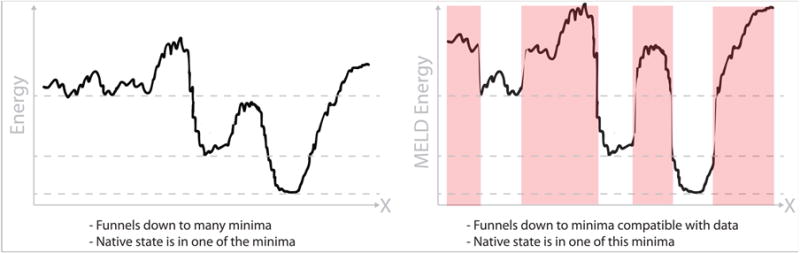
(Left) The energy function given by the forcefield at the lowest replica in a traditional REMD approach. (Right) The same energy function with an arbitrary energy penalty in regions that are not compatible with data (red). MELD uses a one-dimensional replica-exchange ladder approach in which the Hamiltonian and the temperature are both changed together. At the top replica the highest temperature is enforced and the Hamiltonian is the one determined by the forcefield – exactly the same as in a traditional temperature replica exchange approach.

Box 2. Further details of MELD.

Knowledge or data enters into MELD in the form of distance restraints. The restraint energy is given by the following flat-bottomed potential:

$$E(r_{ij})=\{\begin{array}{ll}\frac{1}{2}k(r_1-r_2)(2r_{ij}-r_1-r_2)\hfill & \text{if}{r}_{ij}<r_1\hfill \\ \frac{1}{2}k{(r_{ij}-r_2)}^2\hfill & \text{if}{r}_1\le r_{ij}<r_2\hfill \\ 0\hfill & \text{if}{r}_2\le r_{ij}<r_3\hfill \\ \frac{1}{2}k{(r_{ij}-r_3)}^2\hfill & \text{if}{r}_3\le r_{ij}<r_4\hfill \\ \frac{1}{2}k(r_4-r_3)(2r_{ij}-r_4-r_3)\hfill & \text{if}{r}_4\le r_{ij},\hfill \end{array}$$ (5)

where the coordinates r₁ through r₄ are distance cutoffs delineating the linear, quadratic, and flat regions of the potential, and k is the force constant. Typically the data is broken down into a series of restraining terms between pairs of residues (or atoms in a residue, with distance, r_ij, between two atoms i and j). Agreement with a piece of the data is defined as a distance lying within the flat region of the piecewise function.

MELD can use different possible schemes for scaling the temperature and restraints as the system moves up the replica ladder. But typically the following protocol is followed. First, the temperature is increased with a standard geometric scheme⁸⁶ in the lower replicas and then kept constant at the highest temperature for the remaining replicas, at which point the MELD protocol weakens the restraint term in the Hamiltonian. Restraints are weakened by decreasing the force constant k(n) as a function of replica index, n. The dependence of k on n can take different forms⁶⁴.

The spacing between replicas is adaptive – some automatically increase and some decrease during the equilibration stage of the simulation, to increase the efficiency and avoid sampling bottlenecks^58,64. This is how HT-REMD finds its balance between exploration and exploitation – with exploitation occurring in the lower replicas and exploration in the higher ones.

Figure 3 shows a toy example of how MELD works. We seek the native conformation of a 2-dimensional HP-lattice-model protein. In this model, H-H interactions have a stabilizing energy of 1 unit each. So, in the HP model, finding the native state requires finding the chain conformation(s) having the largest possible number of H-H contacts⁸⁷.

Figure 3. The MELD method explained using a toy HP lattice model.

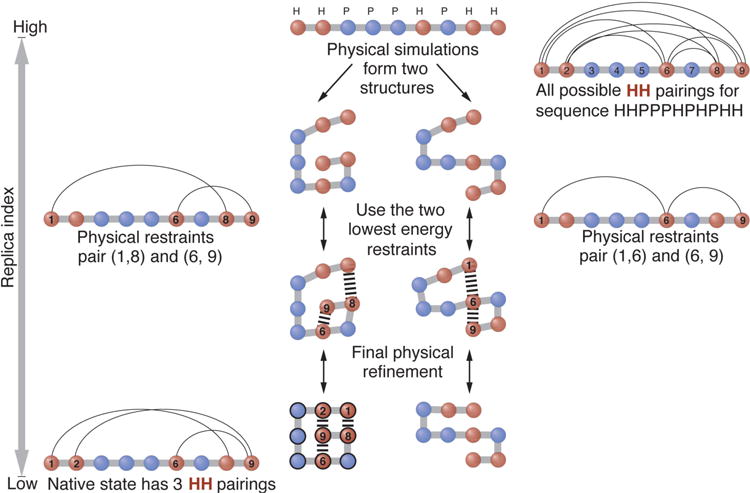
Adapted with permission from A. Perez, J. L. MacCallum, and K. Dill, Proc. Natl. Acad. Sci. U. S. A. 112, 11846 (2015). Copyright 2015 National Academy of Sciences, USA.

Here’s how MELD accelerates finding the native structure of an HP protein. MELD starts by allowing restraints between all possible pairs of H-H residues. However, we know that most of those contacts cannot be satisfied in the native state. Suppose that prior tests have already shown that native HP proteins of this length can usually have only about 2 such contacts. In our REMD ladder, at high-replica index, MELD would sample many possible conformations, and the imposed constraints are weak. A given conformation will now be restrained by the 2 least-stretched H-H interactions available among all possible H-H interactions. At lower replicas, the restraints will be stronger. As the replica ladder is sampled high and low, the restraints tend to drive the conformations to certain subregions of conformational space. In this way, a chain that is in a conformation consistent with the ‘right’ two H-H contacts (i.e. the native contacts) will be found much more efficiently than without having used that information. Since there is no energy bias inside conformational envelopes (because the restraint potentials are zero inside those envelopes), the relative state populations are reflective of the original forcefield. Below, we show some applications of MELD in protein modeling.

Application: Determining protein structures by MELDing experimental data with MD simulations

Much of what’s known about proteins comes from insights gleaned from their native conformations. The PDB now holds over 130,000 atomically detailed biomolecule structures. These structures were obtained from experiments such as X-ray crystallography and NMR. The experimental data alone is often insufficient to fully specify a structure; details must be filled in by computational modeling. The problem is that experimental data has limitations of various types. For example, in solid state NMR, the problem is the sparsity of data. The amount of information is about 0.4 restraints per amino acid, whereas solution-phase NMR gives between 10 and 20 restraints per amino acid. In the former case, physical modeling can fill in where information is insufficient.

Another problem with data is noise and errors. Figure 4 shows an example. This is a situation that uses so-called evolutionary information^88,89. The goal is to infer the structure of a target protein by comparing many different sequences of other proteins that are evolutionarily related to the target. These sequence comparisons are used to draw inferences about which pairs of amino acids might be in contact with each other in the target protein. The problem is that not all the inferred pairings are correct. However, this data can be used with MELD, in short simulations (less than 1 μsec) to give reasonably accurate determinations of the true native structure. Evolutionary sequence modeling is of growing value because of the explosive growth in databases of sequences^90,91.

Figure 4. MELD can make accurate predictions starting from sequence using noisy data.

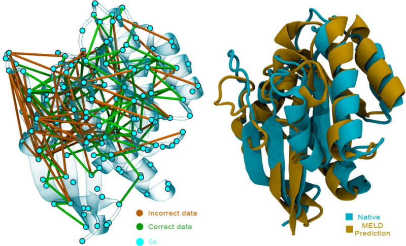
The figure shows evolutionary data from EvFold superposed on the native structure (left) and our top prediction with this data superposed on the native structure (PDBid 5P21) (right).

Application: Predicting protein structures by MELDing guidance from generic physical principles with MD simulations

We often want to predict the native structure of a protein molecule from its amino acid sequence. Unlike the situations above, here, no experimental data is available. But, some general features of native structures are known. Small soluble native proteins have hydrophobic cores, much secondary structure, and are usually fairly compact. We want to instruct a computer to satisfy these Coarse Physical Insights (CPI) while seeking the state of lowest free energy in an MD simulation with a forcefield. We want to impose directives such as: “make a hydrophobic core” (see figures 3 and 5) or “pair up β-strands through hydrogen bonding”. The problem is that these directives are highly ambiguous and combinatoric. There are huge numbers of protein structures having secondary structures, hydrophobic clustering and compactness. The great majority of the specific instances of these directives will be wrong, and only a few will be right. We don’t know which is which a priori. For example, for proteins shorter than 100 residues, typically around 8% of the possible hydrophobic pairing restraints are realized in the native state. If 20 residues were hydrophobic, there would be ≈ 20² = 400 pairwise restraints, only about 32 of which will occur in the native state. However, this kind of information can be used by MELD. MELD has been shown to utilize these kinds of directives to fold most of a test set of 20 small proteins, and do so orders of magnitude faster than the underlying MD could have done alone⁵⁸. Figure 6 shows the scaling of the acceleration resulting from harnessing CPIs in protein folding^37,58,92 compared to brute-force MD³⁷.

Figure 5. Coarse Physical Insights based on hydrophobic residues.

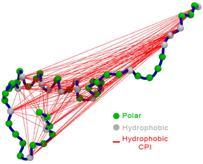
All possible hydrophobic restraints are shown for a structured sampled at high Temperature in a MELD simulation. Only a subset of these (the ones with the lowest restraint energy) will be used to guide the structure to the next time step.

Figure 6. MELD speeds up folding simulations.

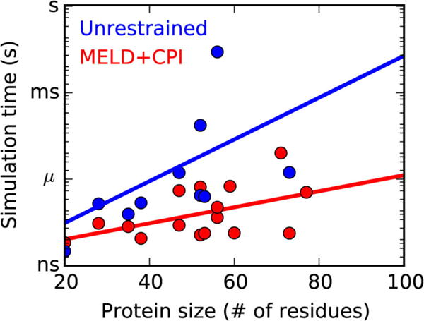
Simulation time required to sample native states starting from fully unfolded states. Adapted with permission from reference⁹²

Application: Predicting native protein structures blindly in the CASP 11 event

MELD is fast enough for prospective tests in a blind structure-prediction competition called CASP^93,94. CASP is a communal event. It begins when the CASP team releases a target protein sequence that has an unknown structure to a wide community of predictors. Nearly 200 predictor groups then attempt to predict its structure, with a 3-week deadline. After the predictions are submitted, the CASP team compares the submissions against each other, and against the true structure, which had been known by the CASP team, but withheld from the predictors. The 3-week deadline has previously been too tight to be met by physics-based simulations, except for the coarse-grained method called UNRES⁶⁷. However, MELD has been able to meet these speed requirements for small proteins. MELD predicted 3 structures with excellent accuracy, based on CPIs, in CASP11 (see Fig. 7)⁶⁶. Furthermore, a different CASP test provides target proteins for which sparse and ambiguous information representing unassigned NMR-like data was given along with the sequence. For 3 such targets, MELD produced the best predictions⁶⁶. Figure 8 summarizes MELD’s success in CASP11 compared to average performance of the field and Rosetta⁵⁰, one of the most successful methods for structure prediction⁹⁵, for the subset of proteins MELD attempted. The figure shows that with MELD acceleration, HT-REMD simulations are promising for predicting protein structures that have previously been difficult for bioinformatics methods.

Figure 7. Blind predictions from CASP 11.

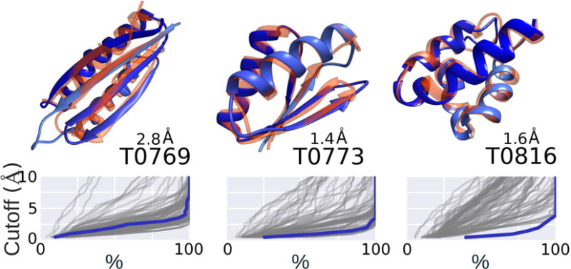
TOP: The name of the targets are denoted according to CASP numbering T0 and can be accessed through http://www.predictioncenter.org. We are the “Laufer” group (number 428). The number on top of the name is the RMSD of our number one submission: centroid structure of the highest population cluster from MELD trajectories. BOTTOM: Hubbard plots¹¹⁵ representing our prediction accuracy (blue) compared to predictions by all other groups in CASP (grey lines). The best results are shown by the shoulder in the line (where the slope changes upwards) being more to the right and low RMSD values (higher % of the structure being less than X Å away from native). Adapted from reference⁶⁶.

Figure 8. The CASP blind test of protein structure prediction.

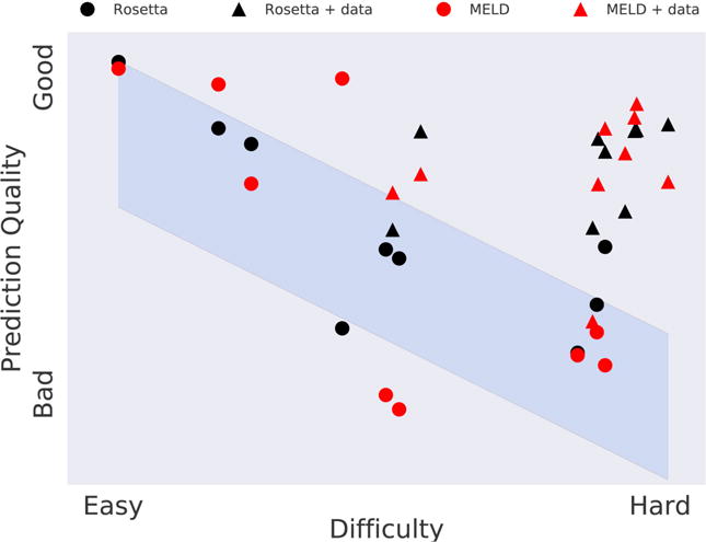
The x-axis represents the degree to which known proteins can be used as starting models for predicting target protein structure. Blue band represents the historical average over 20 years of CASP events, showing that bioinformatics methods have been challenged to predict protein structures. The triangles shows that, when given some additional information beyond the amino-acid sequence, the MELD physical method (black triangles) gives comparable predictions to the best bioinformatics methods (one of which is Rosetta, red triangles).

Application: Predicting the binding poses and affinities of peptides to proteins

MELD is also useful for computing how flexible ligands bind to proteins^96,97. Peptides are relatively flexible and large compared to other ligands, so they have been computationally challenging to simulate with physical methods. We applied MELD to study the binding of a set of peptides to P53 regulators MDM2 and MDMX^96,97. The P53 inhibition of MDM2 and MDMX is a target for anti-cancer therapies^98,99. In this case, the restraints imposed were that the peptide should make hydrophobic contacts in the protein, and that the peptide should be constrained to a spherical shell sufficiently far away so that it can be considered to be non-interacting with the protein-peptide complex; see Figure 9. In the high-temperature replicas, these restraints are weak. The replica exchange process models the binding and unbinding process of these intrinsically disordered peptides into the binding groove^100–105. In the limit of good sampling, MELD gives the populations of different binding modes, and thus the relative binding free energies.

Figure 9. Swapping the different peptides (red and blue) in and out of the protein binding site.

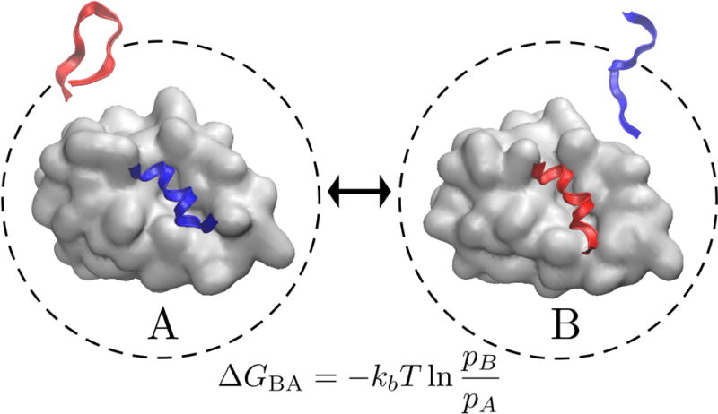
Two possible states (A) in which one peptide (blue structure) is bound to the target protein (gray surface) and the other (red structure) is kept unbound and (B) in which the roles of the peptides are reversed. Each peptide may favor different binding modes. The ratio of the populations between these two cases p_B/p_A can be related to the relative free energy of binding by the equation given here.

Continuing challenges in protein modeling

There remain substantial barriers to searching and sampling in protein modeling. First, there is a need to model larger proteins. Physical modeling falls far short of modeling the average human protein (which has around 450 residues¹⁰⁶). Second, there is a need to model multi-domain proteins⁵⁹ (domains are parts of a protein that tend to be 200 residues or less in size). Third, there is a need to model larger conformational motions and actions in proteins. Fourth, similar needs apply to modeling protein-protein interactions or flexible and disordered regions in proteins.

A key challenge is how to balance the explore vs. exploit components for high efficiency. Where explore-exploit is used in molecular physics, the critical quantity is the temperature, the variable that controls the balance between more exploring (at higher temperatures) vs. more exploiting (at lower temperatures). Many of the methods listed above (simulated annealing, replica exchange) do not rely only on a single balance point (i.e. a single temperature), but rather they define whole ‘temporal’ programs, i.e. procedures for increasing and decreasing the temperature during a simulation. In short, getting the right balance between explore and exploit is a major challenge for computational decision-making with uncertainty, and the optimal balancing strategy can be very different from one class of problem to the next.

New types of external information could be harnessed. One approach has been to harness human intuition, for example in a protein-folding puzzle-solving game called FoldIt^107,107. Also, going forward, the field of protein modeling might benefit from the rapid advances being made in the area of deep-learning, such as in language translation or games such as chess or Go (see Box 3). However, we also note that the reverse is also possible: possibly new methods in protein modeling could add value to other combinatorial search problems. Figure 10 makes two points. First, it shows the progress over time in solving increasingly larger combinatorial problems in different spheres. And second, it shows that the most important problems we face of protein folding are combinatorially at least as challenging as those of games. Roughly, the number of positions in games (V = 10⁵⁰ in chess and V = 10¹⁷⁰ in Go) can be compared to the number of possible backbone dihedral states for an N-residue protein (V = 3^(2N−2)). If we follow the standard Levinthal argument¹⁰⁸, the conformational volume in all three cases is too large to sample exhaustively. It has taken nearly 20 years to go from folding the villin headpiece (35 residues, V = 10³²) to the λ-repressor (92 residues, V = 10⁸⁶) with MD. Physics-based predictions of the structures of proteins that are 300-residues long (10²⁸⁵) is not likely to be accomplished simply by faster computers. It is important to develop new algorithmic approaches to exploring and exploiting that can take advantage of knowledge or intuition.

Box 3. Opportunities for cross-fertilization with other explore-and-exploit problems.

Exploring and exploiting are widely used in computational optimization, such as the following:

Industrial and scientific innovation

Companies aim to balance their investments in exploring (seeking new growth opportunities or new features, or research, development, innovation and the invention of new products) vs. exploiting (supporting and improving existing products and businesses). The high failure rates of technology companies has been attributed to improper balancing of EE, called ‘Organizational ambidexterity’¹⁰⁹ – it is said that only about 2 % of companies find the right balance¹¹⁰. The successes of basic research, in Bell Labs and General Electric, has been attributed to their emphasis on ‘idle curiosity’¹¹¹, the exploration component.

Computational gaming

Computer chess is an explore-exploit problem. In 1997, IBM’s Deep Blue computer algorithm defeated chess master Gary Kasparov. Deep Blue’s algorithm³ was mainly a brute-force tree-search method that could look ahead ≈ 12 moves in three minutes. The basic objective function in chess is that each piece has a particular value. However, Deep Blue also made use of some heuristics derived by chess masters that could modify the values of pieces given a particular layout. Hence, the algorithm explored exhaustively all possible moves to a given depth and then exploited the ones with the highest scores.

The board game GO is regarded as more complex than chess. Its number of legal configurations¹¹² is 10¹⁷⁰(compared to 10⁵⁰ in chess^113,114) and there is no clear mapping to a scoring function for each decision. It requires a more global ‘gestalt’. In a remarkable recent success, Google DeepMind’s⁴ computational method called αGo defeated human grandmaster Lee Sedol. The solution was a balance between exploring and exploiting based on the use of a Monte Carlo Tree Search (MCTS), combined with deep learning from playing large numbers of prior games.

Figure 10. Search space increases exponentially with protein size.

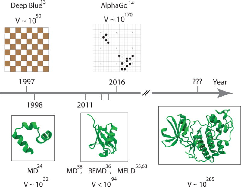
Bigger computers alone have not been the solution to the game of Go nor to protein folding. Alternative algorithms that can incorporate intuition and current knowledge can help improve the scaling⁹².

References

- 1.Toth Z, Kalnay E. Ensemble forecasting at NCEP and the breeding method. Monthly Weather Review. 1997;125(12):3297–3319. [Google Scholar]
- 2.Molteni F, Buizza R, Palmer TN, Petroliagis T. The ECMWF ensemble prediction system: Methodology and validation. Quarterly Journal of the Royal Meteorological Society. 1996;122(529):73–119. [Google Scholar]
- 3.Campbell M, Hoane AJ, Hsu FH. Deep Blue. Artificial Intelligence. 2002;134(1):57–83. [Google Scholar]
- 4.Silver D, Huang A, Maddison CJ, Guez A, Sifre L, van den Driessche G, et al. Mastering the game of Go with deep neural networks and tree search. Nature. 2016;529(7587):484–489. doi: 10.1038/nature16961. [DOI] [PubMed] [Google Scholar]
- 5.Metropolis N, Rosenbluth AW, Rosenbluth MN, Teller AH, Teller E. Equation of State Calculations by Fast Computing Machines. The Journal of chemical physics. 1953;21(6):1087–1092. [Google Scholar]
- 6.Hansmann UHE, Okamoto Y. New Monte Carlo algorithms for protein folding. Current opinion in structural biology. 1999;9(2):177–183. doi: 10.1016/S0959-440X(99)80025-6. [DOI] [PubMed] [Google Scholar]
- 7.McCammon JA, Gelin BR, Karplus M. Dynamics of folded proteins. Nature. 1977;267(5612):585–590. doi: 10.1038/267585a0. [DOI] [PubMed] [Google Scholar]
- 8.Sugita Y, Okamoto Y. Replica-exchange molecular dynamics method for protein folding. Chemical Physics Letters. 1999;314(1–2):141–151. [Google Scholar]
- 9.Okamoto Y. Generalized-ensemble algorithms: enhanced sampling techniques for Monte Carlo and molecular dynamics simulations. Journal of Molecular Graphics and Modelling. 2004;22(5):425–439. doi: 10.1016/j.jmgm.2003.12.009. [DOI] [PubMed] [Google Scholar]
- 10.Torrie GM, Valleau JP. Nonphysical sampling distributions in Monte Carlo free-energy estimation: Umbrella sampling. Journal of Computational Physics. 1977;23(2):187–199. [Google Scholar]
- 11.Lu H, Isralewitz B, Krammer A, Vogel V, Schulten K. Unfolding of titin immunoglobulin domains by steered molecular dynamics simulation. Biophysical journal. 1998;75(2):662–671. doi: 10.1016/S0006-3495(98)77556-3. [DOI] [PMC free article] [PubMed] [Google Scholar]
- 12.Laio A, Parrinello M. Escaping free-energy minima. Proceedings of the National Academy of Sciences of the United States of America. 2002;99(20):12562–12566. doi: 10.1073/pnas.202427399. [DOI] [PMC free article] [PubMed] [Google Scholar]
- 13.Khachaturyan A, Semenovskaya S, Vainstein B. A Statistical-Thermodynamic Approach to Determination of Structure Amplitude Phases. Sov Phys Crystallogr. 1979;24:519–524. [Google Scholar]
- 14.Holland J. Adaptation in natural and artificial systems. Cambridge CA: MIT press; 1975. [Google Scholar]
- 15.Berger-Tal O, Nathan J, Meron E, Saltz D. The exploration-exploitation dilemma: a multidisciplinary framework. PLoS One. 2014;9(4):e95693. doi: 10.1371/journal.pone.0095693. [DOI] [PMC free article] [PubMed] [Google Scholar]
- 16.Christen M, van Gunsteren WF. On searching in, sampling of, and dynamically moving through conformational space of biomolecular systems: A review. Journal of Computational Chemistry. 2008;29(2):157–166. doi: 10.1002/jcc.20725. [DOI] [PubMed] [Google Scholar]
- 17.Zimmerman MI, Bowman GR. FAST Conformational Searches by Balancing Exploration/Exploitation Trade-Offs. Journal of chemical theory and computation. 2015;11(12):5747–5757. doi: 10.1021/acs.jctc.5b00737. [DOI] [PubMed] [Google Scholar]
- 18.Daw ND, O’Doherty JP, Dayan P, Seymour B, Dolan RJ. Cortical substrates for exploratory decisions in humans. Nature. 2006;441(7095):876–879. doi: 10.1038/nature04766. [DOI] [PMC free article] [PubMed] [Google Scholar]
- 19.Katehakis MN, Arthur F, Veinott J. The Multi-Armed Bandit Problem: Decomposition and Computation. Mathematics of Operations Research. 1987;12(2):262–268. [Google Scholar]
- 20.Gittins JC. Bandit Processes and Dynamic Allocation Indexes. Journal of the Royal Statistical Society Series B-Methodological. 1979;41(2):148–177. [Google Scholar]
- 21.Berry DA, Fristedt B. Bandit problems Sequential Allocation of Experiments. Springer; 2014. [Google Scholar]
- 22.Dill KA, Chan HS. From Levinthal to pathways to funnels. Nature structural biology. 1997;4(1):10–19. doi: 10.1038/nsb0197-10. [DOI] [PubMed] [Google Scholar]
- 23.Levinthal C. Molecular model-building by computer. Scientific American. 1966;214(6):42–52. doi: 10.1038/scientificamerican0666-42. [DOI] [PubMed] [Google Scholar]
- 24.Levitt M, Warshel A. Computer-Simulation of Protein Folding. Nature. 1975;253(5494):694–698. doi: 10.1038/253694a0. [DOI] [PubMed] [Google Scholar]
- 25.Duan Y, Kollman PA. Pathways to a protein folding intermediate observed in a 1-microsecond simulation in aqueous solution. Science (New York, NY) 1998;282(5389):740–744. doi: 10.1126/science.282.5389.740. [DOI] [PubMed] [Google Scholar]
- 26.Maier JA, Martinez C, Kasavajhala K, Wickstrom L, Hauser KE, Simmerling C. ff14SB: Improving the Accuracy of Protein Side Chain and Backbone Parameters from ff99SB. Journal of chemical theory and computation. 2015;11(8):3696–3713. doi: 10.1021/acs.jctc.5b00255. [DOI] [PMC free article] [PubMed] [Google Scholar]
- 27.Lindorff-Larsen K, Piana S, Palmo K, Maragakis P, Klepeis JL, Dror RO, et al. Improved side-chain torsion potentials for the Amber ff99SB protein force field. Proteins. 2010;78(8):1950–1958. doi: 10.1002/prot.22711. [DOI] [PMC free article] [PubMed] [Google Scholar]
- 28.Best RB, Zhu X, Shim J, Lopes PEM, Mittal J, Feig M, et al. Optimization of the additive CHARMM all-atom protein force field targeting improved sampling of the backbone φ, ψ and side-chain χ(1) and χ(2) dihedral angles. Journal of chemical theory and computation. 2012;8(9):3257–3273. doi: 10.1021/ct300400x. [DOI] [PMC free article] [PubMed] [Google Scholar]
- 29.MacKerell AD, Feig M, Brooks CL. Extending the treatment of backbone energetics in protein force fields: Limitations of gas-phase quantum mechanics in reproducing protein conformational distributions in molecular dynamics simulations. Journal of Computational Chemistry. 2004;25(11):1400–1415. doi: 10.1002/jcc.20065. [DOI] [PubMed] [Google Scholar]
- 30.MacKerell AD, Feig M, Brooks CL. Improved treatment of the protein backbone in empirical force fields. Journal of the American Chemical Society. 2004;126(3):698–699. doi: 10.1021/ja036959e. [DOI] [PubMed] [Google Scholar]
- 31.Hornak V, Abel R, Okur A, Strockbine B, Roitberg A, Simmerling C. Comparison of multiple Amber force fields and development of improved protein backbone parameters. Proteins. 2006;65(3):712–725. doi: 10.1002/prot.21123. [DOI] [PMC free article] [PubMed] [Google Scholar]
- 32.Perez A, MacCallum JL, Brini E, Simmerling C, Dill K. Grid-based backbone correction to the ff12SB protein force field for implicit-solvent simulations. Journal of chemical theory and computation. 2015;11(10):4770–4779. doi: 10.1021/acs.jctc.5b00662. [DOI] [PMC free article] [PubMed] [Google Scholar]
- 33.Nguyen H, Roe DR, Simmerling C. Improved Generalized Born Solvent Model Parameters for Protein Simulations. Journal of chemical theory and computation. 2013;9(4):2020–2034. doi: 10.1021/ct3010485. [DOI] [PMC free article] [PubMed] [Google Scholar]
- 34.Shaw DE, Deneroff MM, Dror RO, Salmon JK, Batson B, Bowers KJ, et al. Anton, a special-purpose machine for molecular dynamics simulation. ACM SIGARCH Computer Architecture News. 2007;35(2):1–12. [Google Scholar]
- 35.Götz AW, Williamson MJ, Xu D, Poole D, Le Grand S, Walker RC. Routine Microsecond Molecular Dynamics Simulations with AMBER on GPUs. 1. Generalized Born. Journal of chemical theory and computation. 2012;8(5):1542–1555. doi: 10.1021/ct200909j. [DOI] [PMC free article] [PubMed] [Google Scholar]
- 36.Freddolino PL, Liu F, Gruebele M, Schulten K. Ten-microsecond molecular dynamics simulation of a fast-folding WW domain. Biophysical journal. 2008;94(10):L75–7. doi: 10.1529/biophysj.108.131565. [DOI] [PMC free article] [PubMed] [Google Scholar]
- 37.Nguyen H, Maier J, Huang H, Perrone V, Simmerling C. Folding simulations for proteins with diverse topologies are accessible in days with a physics-based force field and implicit solvent. Journal of the American Chemical Society. 2014;136(40):13959–13962. doi: 10.1021/ja5032776. [DOI] [PMC free article] [PubMed] [Google Scholar]
- 38.Voelz VA, Bowman GR, Beauchamp K, Pande VS. Molecular simulation of ab initio protein folding for a millisecond folder NTL9(1–39) Journal of the American Chemical Society. 2010;132(5):1526–1528. doi: 10.1021/ja9090353. [DOI] [PMC free article] [PubMed] [Google Scholar]
- 39.Lindorff-Larsen K, Piana S, Dror RO, Shaw DE. How fast-folding proteins fold. Science (New York, NY) 2011;334(6055):517–520. doi: 10.1126/science.1208351. [DOI] [PubMed] [Google Scholar]
- 40.Zagrovic B, Snow CD, Shirts MR, Pande VS. Simulation of Folding of a Small Alpha-helical Protein in Atomistic Detail using Worldwide-distributed Computing. Journal of molecular biology. 2002;323(5):927–937. doi: 10.1016/s0022-2836(02)00997-x. [DOI] [PubMed] [Google Scholar]
- 41.Seibert MM, Patriksson A, Hess B, van der Spoel D. Reproducible Polypeptide Folding and Structure Prediction using Molecular Dynamics Simulations. Journal of molecular biology. 2005;354(1):173–183. doi: 10.1016/j.jmb.2005.09.030. [DOI] [PubMed] [Google Scholar]
- 42.Piana S, Lindorff-Larsen K, Shaw DE. Protein folding kinetics and thermodynamics from atomistic simulation. Proceedings of the National Academy of Sciences of the United States of America. 2012;109(44):17845–17850. doi: 10.1073/pnas.1201811109. [DOI] [PMC free article] [PubMed] [Google Scholar]
- 43.Shaw DE, Maragakis P, Lindorff-Larsen K, Piana S, Dror RO, Eastwood MP, et al. Atomic-Level Characterization of the Structural Dynamics of Proteins. Science (New York, NY) 2010;330(6002):341–346. doi: 10.1126/science.1187409. [DOI] [PubMed] [Google Scholar]
- 44.Schneidman-Duhovny D, Pellarin R, Sali A. Uncertainty in integrative structural modeling. Current opinion in structural biology. 2014;28:96–104. doi: 10.1016/j.sbi.2014.08.001. [DOI] [PMC free article] [PubMed] [Google Scholar]
- 45.Ward AB, Sali A, Wilson IA. Biochemistry. Integrative structural biology. Science (New York, NY) 2013;339(6122):913–915. doi: 10.1126/science.1228565. [DOI] [PMC free article] [PubMed] [Google Scholar]
- 46.Berman HM, Westbrook J, Feng Z, Gilliland G, Bhat TN, Weissig H, et al. The Protein Data Bank. Nucleic acids research. 2000;28(1):235–242. doi: 10.1093/nar/28.1.235. [DOI] [PMC free article] [PubMed] [Google Scholar]
- 47.Bourne PE, Addess KJ, Bluhm WF, Chen L, Deshpande N, Feng Z, et al. The distribution and query systems of the RCSB Protein Data Bank. Nucleic acids research. 2004;32:D223–5. doi: 10.1093/nar/gkh096. Database issue. [DOI] [PMC free article] [PubMed] [Google Scholar]
- 48.Chothia C, Lesk AM. The Relation Between the Divergence of Sequence and Structure in Proteins. Embo Journal. 1986;5(4):823–826. doi: 10.1002/j.1460-2075.1986.tb04288.x. [DOI] [PMC free article] [PubMed] [Google Scholar]
- 49.Baker D, Sali A. Protein structure prediction and structural genomics. Science (New York, NY) 2001;294(5540):93–96. doi: 10.1126/science.1065659. [DOI] [PubMed] [Google Scholar]
- 50.Simons KT, Bonneau R, Ruczinski I, Baker D. Ab initio protein structure prediction of CASP III targets using ROSETTA. Proteins-Structure Function and Genetics. 1999;(Suppl 3):171–176. doi: 10.1002/(sici)1097-0134(1999)37:3+<171::aid-prot21>3.3.co;2-q. [DOI] [PubMed] [Google Scholar]
- 51.Zhou H, Skolnick J. Ab initio protein structure prediction using chunk-TASSER. Biophysical journal. 2007;93(5):1510–1518. doi: 10.1529/biophysj.107.109959. [DOI] [PMC free article] [PubMed] [Google Scholar]
- 52.Zhang Y, Skolnick J. Automated structure prediction of weakly homologous proteins on a genomic scale. Proceedings of the National Academy of Sciences of the United States of America. 2004;101(20):7594–7599. doi: 10.1073/pnas.0305695101. [DOI] [PMC free article] [PubMed] [Google Scholar]
- 53.Rueda M, Ferrer-Costa C, Meyer T, Perez A, Camps J, Hospital A, et al. A consensus view of protein dynamics. Proceedings of the National Academy of Sciences of the United States of America. 2007;104(3):796–801. doi: 10.1073/pnas.0605534104. [DOI] [PMC free article] [PubMed] [Google Scholar]
- 54.Meyer T, D’Abramo M, Hospital A, Rueda M, Ferrer-Costa C, Perez A, et al. MoDEL (Molecular Dynamics Extended Library): a database of atomistic molecular dynamics trajectories. Structure (London, England: 1993) 2010;18(11):1399–1409. doi: 10.1016/j.str.2010.07.013. [DOI] [PubMed] [Google Scholar]
- 55.Schaeffer RD, Daggett V. Protein folds and protein folding. Protein engineering. 2011;24(1–2):11–19. doi: 10.1093/protein/gzq096. [DOI] [PMC free article] [PubMed] [Google Scholar]
- 56.Day R, Beck DAC, Armen RS, Daggett V. A consensus view of fold space: combining SCOP, CATH, and the Dali Domain Dictionary. Protein science: a publication of the Protein Society. 2003;12(10):2150–2160. doi: 10.1110/ps.0306803. [DOI] [PMC free article] [PubMed] [Google Scholar]
- 57.Mirjalili V, Feig M. Protein Structure Refinement through Structure Selection and Averaging from Molecular Dynamics Ensembles. Journal of chemical theory and computation. 2013;9(2):1294–1303. doi: 10.1021/ct300962x. [DOI] [PMC free article] [PubMed] [Google Scholar]
- 58.Perez A, MacCallum JL, Dill K. Accelerating molecular simulations of proteins using Bayesian inference on weak information. Proceedings of the National Academy of Sciences. 2015;112(38):11846–11851. doi: 10.1073/pnas.1515561112. [DOI] [PMC free article] [PubMed] [Google Scholar]
- 59.Gianni S, Jemth P. Protein folding: Vexing debates on a fundamental problem. Biophysical chemistry. 2016;212:17–21. doi: 10.1016/j.bpc.2016.03.001. [DOI] [PubMed] [Google Scholar]
- 60.Dickson A, Ahlstrom LS, Brooks CL. Coupled folding and binding with 2D Window-Exchange Umbrella Sampling. Journal of Computational Chemistry. 2016;37(6):587–594. doi: 10.1002/jcc.24004. [DOI] [PMC free article] [PubMed] [Google Scholar]
- 61.Miao Y, Feixas F, Eun C, McCammon JA. Accelerated molecular dynamics simulations of protein folding. Journal of Computational Chemistry. 2015;36(20):1536–1549. doi: 10.1002/jcc.23964. [DOI] [PMC free article] [PubMed] [Google Scholar]
- 62.Noé F, Schuette C, Vanden-Eijnden E, Reich L, Weikl TR. Constructing the equilibrium ensemble of folding pathways from short off-equilibrium simulations. Proceedings of the National Academy of Sciences of the United States of America. 2009;106(45):19011–19016. doi: 10.1073/pnas.0905466106. [DOI] [PMC free article] [PubMed] [Google Scholar]
- 63.Beauchamp KA, McGibbon R, Lin YS, Pande VS. Simple few-state models reveal hidden complexity in protein folding. Proceedings of the National Academy of Sciences. 2012;109(44):17807–17813. doi: 10.1073/pnas.1201810109. [DOI] [PMC free article] [PubMed] [Google Scholar]
- 64.MacCallum JL, Perez A, Dill K. Determining protein structures by combining semire-liable data with atomistic physical models by Bayesian inference. Proceedings of the National Academy of Sciences. 2015;112(22):6985–6990. doi: 10.1073/pnas.1506788112. [DOI] [PMC free article] [PubMed] [Google Scholar]
- 65.Su lkowska JI, Noel JK, Onuchic JN. Energy landscape of knotted protein folding. Proceedings of the National Academy of Sciences. 2012;109(44):17783–17788. doi: 10.1073/pnas.1201804109. [DOI] [PMC free article] [PubMed] [Google Scholar]
- 66.Perez A, Morrone JA, Brini E, MacCallum JL, Dill KA. Blind protein structure prediction using accelerated free-energy simulations. accepted in Science Advances. 2016 doi: 10.1126/sciadv.1601274. [DOI] [PMC free article] [PubMed] [Google Scholar]
- 67.Krupa P, Mozolewska MA, Wiśniewska M, Yin Y, He Y, Sieradzan AK, et al. Performance of protein-structure predictions with the physics-based UNRES force field in CASP11. Bioinformatics (Oxford, England) 2016:btw404. doi: 10.1093/bioinformatics/btw404. [DOI] [PMC free article] [PubMed] [Google Scholar]
- 68.Walters BT, Mayne L, Hinshaw JR, Sosnick TR, Englander SW. Folding of a large protein at high structural resolution. Proceedings of the National Academy of Sciences. 2013;110(47):18898–18903. doi: 10.1073/pnas.1319482110. [DOI] [PMC free article] [PubMed] [Google Scholar]
- 69.Hu W, Walters BT, Kan ZY, Mayne L, Rosen LE, Marqusee S, et al. Stepwise protein folding at near amino acid resolution by hydrogen exchange and mass spectrometry. Proceedings of the National Academy of Sciences of the United States of America. 2013;110(19):7684–7689. doi: 10.1073/pnas.1305887110. [DOI] [PMC free article] [PubMed] [Google Scholar]
- 70.Sekhar A, Kay LE. NMR paves the way for atomic level descriptions of sparsely populated, transiently formed biomolecular conformers. Proceedings of the National Academy of Sciences. 2013;110(32):12867–12874. doi: 10.1073/pnas.1305688110. [DOI] [PMC free article] [PubMed] [Google Scholar]
- 71.Rauscher S, Gapsys V, Gajda MJ, Zweckstetter M, de Groot BL, Grubmüller H. Structural Ensembles of Intrinsically Disordered Proteins Depend Strongly on Force Field: A Comparison to Experiment. Journal of chemical theory and computation. 2015;11(11):5513–5524. doi: 10.1021/acs.jctc.5b00736. [DOI] [PubMed] [Google Scholar]
- 72.Piana S, Donchev AG, Robustelli P, Shaw DE. Water Dispersion Interactions Strongly Influence Simulated Structural Properties of Disordered Protein States. The journal of physical chemistry B. 2015;119(16):5113–5123. doi: 10.1021/jp508971m. [DOI] [PubMed] [Google Scholar]
- 73.Kirshenbaum K, Barron AE, Goldsmith RA, Armand P, Bradley EK, Truong KTV, et al. Sequence-specific polypeptoids: A diverse family of heteropolymers with stable secondary structure. Proceedings of the National Academy of Sciences of the United States of America. 1998;95(8):4303–4308. doi: 10.1073/pnas.95.8.4303. [DOI] [PMC free article] [PubMed] [Google Scholar]
- 74.Sborgi L, Verma A, Piana S, Lindorff-Larsen K, Cerminara M, Santiveri CM, et al. Interaction Networks in Protein Folding via Atomic-Resolution Experiments and Long-Time-Scale Molecular Dynamics Simulations. Journal of the American Chemical Society. 2015;137(20):6506–6516. doi: 10.1021/jacs.5b02324. [DOI] [PMC free article] [PubMed] [Google Scholar]
- 75.Shen Y, Lange O, Delaglio F, Rossi P, Aramini JM, Liu G, et al. Consistent blind protein structure generation from NMR chemical shift data. Proceedings of the National Academy of Sciences. 2008;105(12):4685–4690. doi: 10.1073/pnas.0800256105. [DOI] [PMC free article] [PubMed] [Google Scholar]
- 76.De Simone A, Montalvao RW, Vendruscolo M. Determination of Conformational Equilibria in Proteins Using Residual Dipolar Couplings. Journal of chemical theory and computation. 2011;7(12):4189–4195. doi: 10.1021/ct200361b. [DOI] [PMC free article] [PubMed] [Google Scholar]
- 77.Esteban-Martín S, Bryn Fenwick R, Salvatella X. Synergistic use of NMR and MD simulations to study the structural heterogeneity of proteins. Wiley Interdisciplinary Reviews: Computational Molecular Science. 2012;2(3):466–478. [Google Scholar]
- 78.Mantsyzov AB, Shen Y, Lee JH, Hummer G, Bax A. MERA: a webserver for evaluating backbone torsion angle distributions in dynamic and disordered proteins from NMR data. Journal of biomolecular NMR. 2015;63(1):85–95. doi: 10.1007/s10858-015-9971-2. [DOI] [PMC free article] [PubMed] [Google Scholar]
- 79.Hummer G, Köfinger J. Bayesian ensemble refinement by replica simulations and reweighting. The Journal of chemical physics. 2015;143(24):243150. doi: 10.1063/1.4937786. [DOI] [PubMed] [Google Scholar]
- 80.Granata D, Camilloni C, Vendruscolo M, Laio A. Characterization of the free-energy landscapes of proteins by NMR-guided metadynamics. Proceedings of the National Academy of Sciences of the United States of America. 2013;110(17):6817–6822. doi: 10.1073/pnas.1218350110. [DOI] [PMC free article] [PubMed] [Google Scholar]
- 81.Laio A, Gervasio FL. Metadynamics: a method to simulate rare events and reconstruct the free energy in biophysics, chemistry and material science. Reports on Progress in Physics. 2008;71(12):126601. [Google Scholar]
- 82.Bonomi M, Camilloni C, Cavalli A, Vendruscolo M. Metainference: A Bayesian inference method for heterogeneous systems. Science Advances. 2016;2(1):e1501177–e1501177. doi: 10.1126/sciadv.1501177. [DOI] [PMC free article] [PubMed] [Google Scholar]
- 83.Singharoy A, Teo I, McGreevy R, Stone JE, Zhao J, Schulten K. Molecular dynamics-based model refinement and validation for sub-5 angstrom cryo-electron microscopy maps. eLife. 2016:5. doi: 10.7554/eLife.16105. [DOI] [PMC free article] [PubMed] [Google Scholar]
- 84.McGreevy R, Teo I, Singharoy A, Schulten K. Advances in the molecular dynamics flexible fitting method for cryo-EM modeling. Methods (San Diego, Calif) 2016;100:50–60. doi: 10.1016/j.ymeth.2016.01.009. [DOI] [PMC free article] [PubMed] [Google Scholar]
- 85.Trabuco LG, Villa E, Mitra K, Frank J, Schulten K. Flexible Fitting of Atomic Structures into Electron Microscopy Maps Using Molecular Dynamics. Structure (London, England: 1993) 2008;16(5):673–683. doi: 10.1016/j.str.2008.03.005. [DOI] [PMC free article] [PubMed] [Google Scholar]
- 86.Kofke DA. On the acceptance probability of replica-exchange Monte Carlo trials. The Journal of chemical physics. 2002;117(15):6911–6914. [Google Scholar]
- 87.Lau KF, Dill K. A lattice statistical mechanics model of the conformational and sequence spaces of proteins. Macromolecules. 1989;22(10):3986–3997. [Google Scholar]
- 88.Marks DS, Colwell LJ, Sheridan R, Hopf TA, Pagnani A, Zecchina R, et al. Protein 3D structure computed from evolutionary sequence variation. PLoS One. 2011;6(12):e28766. doi: 10.1371/journal.pone.0028766. [DOI] [PMC free article] [PubMed] [Google Scholar]
- 89.Jones DT, Buchan DWA, Cozzetto D, Pontil M. PSICOV: precise structural contact prediction using sparse inverse covariance estimation on large multiple sequence alignments. Bioinformatics (Oxford, England) 2012;28(2):184–190. doi: 10.1093/bioinformatics/btr638. [DOI] [PubMed] [Google Scholar]
- 90.Wang S, Sun S, Li Z, Zhang R, Xu J. Accurate De Novo Prediction of Protein Contact Map by Ultra-Deep Learning Model. PLoS computational biology. 2017;13(1):e1005324. doi: 10.1371/journal.pcbi.1005324. [DOI] [PMC free article] [PubMed] [Google Scholar]
- 91.Ovchinnikov S, Park H, Varghese N, Huang PS, Pavlopoulos GA, Kim DE, et al. Protein structure determination using metagenome sequence data. Science (New York, NY) 2017;355(6322):294–298. doi: 10.1126/science.aah4043. [DOI] [PMC free article] [PubMed] [Google Scholar]
- 92.Perez A, Morrone JA, Simmerling C, Dill K. Advances in free-energy-based simulations of protein folding and ligand binding. Current opinion in structural biology. 2016;36:25–31. doi: 10.1016/j.sbi.2015.12.002. [DOI] [PMC free article] [PubMed] [Google Scholar]
- 93.Moult J, Pedersen JT, Judson R, Fidelis K. A large-scale experiment to assess protein structure prediction methods. Proteins-Structure Function and Genetics. 1995;23(3):ii–v. doi: 10.1002/prot.340230303. [DOI] [PubMed] [Google Scholar]
- 94.Moult J, Fidelis K, Kryshtafovych A, Schwede T, Tramontano A. Critical assessment of methods of protein structure prediction (CASP) - round x. Proteins. 2013;82(S2):1–6. doi: 10.1002/prot.24452. [DOI] [PMC free article] [PubMed] [Google Scholar]
- 95.Ovchinnikov S, Kinch L, Park H, Liao Y, Pei J, Kim DE, et al. Large-scale determination of previously unsolved protein structures using evolutionary information. eLife. 2015;4:e09248. doi: 10.7554/eLife.09248. [DOI] [PMC free article] [PubMed] [Google Scholar]
- 96.Morrone JA, Perez A, Deng Q, Ha SN, Holloway MK, Sawyer TK, et al. Molecular Simulations Identify Binding Poses and Approximate Affinities of Stapled α-Helical Peptides to MDM2 and MDMX. Journal of chemical theory and computation. 2017;13(2):863–869. doi: 10.1021/acs.jctc.6b00978. [DOI] [PubMed] [Google Scholar]
- 97.Morrone JA, Perez A, MacCallum J, Dill K. Computed Binding of Peptides to Proteins with MELD-Accelerated Molecular Dynamics. Journal of chemical theory and computation. 2017;13(2):870–876. doi: 10.1021/acs.jctc.6b00977. [DOI] [PubMed] [Google Scholar]
- 98.Hoe KK, Verma CS, Lane DP. Drugging the p53 pathway: understanding the route to clinical efficacy. Nature Reviews Drug Discovery. 2014;13(3):217–236. doi: 10.1038/nrd4236. [DOI] [PubMed] [Google Scholar]
- 99.Chène P. Inhibition of the p53-MDM2 interaction: targeting a protein-protein interface. Molecular Cancer Research. 2004;2(1):20–28. [PubMed] [Google Scholar]
- 100.Phan J, Li Z, Kasprzak A, Li B, Sebti S, Guida W, et al. Structure-based Design of High Affinity Peptides Inhibiting the Interaction of p53 with MDM2 and MDMX. Journal of Biological Chemistry. 2010;285(3):2174–2183. doi: 10.1074/jbc.M109.073056. [DOI] [PMC free article] [PubMed] [Google Scholar]
- 101.Baek S, Kutchukian PS, Verdine GL, Huber R, Holak TA, Lee KW, et al. Structure of the Stapled p53 Peptide Bound to Mdm2. Journal of the American Chemical Society. 2011;134(1):103–106. doi: 10.1021/ja2090367. [DOI] [PubMed] [Google Scholar]
- 102.Chang YS, Graves B, Guerlavais V, Tovar C, Packman K, To KH, et al. Stapled α-helical peptide drug development: a potent dual inhibitor of MDM2 and MDMX for p53-dependent cancer therapy. Proceedings of the National Academy of Sciences. 2013;110(36):E3445–54. doi: 10.1073/pnas.1303002110. [DOI] [PMC free article] [PubMed] [Google Scholar]
- 103.Guerlavais V, Darlak K, Sawyer TK, Chang YS, Graves B, Tovar C, et al. Design, Synthesis, Biophysical and Structure-Activity Properties of a Novel Dual MDM2 and MDMX Targeting Stapled α-Helical Peptide: ATSP-7041 Exhibits Potent In Vitro and In Vivo Efficiay in Xenograft Models of Human Cancer. Proceedings of the rd American Peptide Symposium. 2013:184–185. [Google Scholar]
- 104.Shin JS, Ha JH, Lee DH, Ryu KS, Bae KH, Park BC, et al. Structural convergence of unstructured p53 family transactivation domains in MDM2 recognition. Cell cycle (Georgetown, Tex) 2015;14(4):533–543. doi: 10.1080/15384101.2014.998056. [DOI] [PMC free article] [PubMed] [Google Scholar]
- 105.Pazgier M, Liu M, Zou G, Yuan W, Li C, Li C, et al. Structural basis for high-affinity peptide inhibition of p53 interactions with MDM2 and MDMX. Proceedings of the National Academy of Sciences. 2009;106(12):4665–4670. doi: 10.1073/pnas.0900947106. [DOI] [PMC free article] [PubMed] [Google Scholar]
- 106.Hendil KB, Hartmann-Petersen R, Tanaka K. 26 S proteasomes function as stable entities. Journal of molecular biology. 2002;315(4):627–636. doi: 10.1006/jmbi.2001.5285. [DOI] [PubMed] [Google Scholar]
- 107.Cooper S, Khatib F, Treuille A, Barbero J, Lee J, Beenen M, et al. Predicting protein structures with a multiplayer online game. Nature. 2010;466(7307):756–760. doi: 10.1038/nature09304. [DOI] [PMC free article] [PubMed] [Google Scholar]
- 108.Levinthal C. How to fold graciously. Mossbauer spectroscopy in biological systems. 1969;67:22–24. [Google Scholar]
- 109.O’Reilly CA, Tushman ML. Organizational Ambidexterity in Action: How Managers Explore and Exploit. California Management Review. 2011;53(4):5–22. [Google Scholar]
- 110.Reeves M, Haanaes K, Sinha J. How to Choose and Execute the Right Approach. Harvard Business Review Press; 2015. Your Strategy Needs a Strategy. [Google Scholar]
- 111.Gertner J. Bell Labs and the Great Age of American Innovation. Penguin; 2013. The Idea Factory. [Google Scholar]
- 112.Tromp J, Farnebäck G. Computers and Games. Berlin, Heidelberg: Springer Berlin Heidelberg; 2006. Combinatorics of Go; pp. 84–99. [Google Scholar]
- 113.Shannon CE. XXII. Programming a computer for playing chess. The London, Edin-burgh, and Dublin Philosophical Magazine and Journal of Science. 1950;41(314):256–275. [Google Scholar]
- 114.Allis LV. Searching for Solutions in Games and Artificial Intelligence. 1994 [Google Scholar]
- 115.Hubbard TJP. RMS/Coverage graphs: A qualitative method for comparing three-dimensional protein structure predictions. Proteins. 1998;37(S3):15–21. doi: 10.1002/(sici)1097-0134(1999)37:3+<15::aid-prot4>3.3.co;2-q. [DOI] [PubMed] [Google Scholar]