EMPOWERING CORTICAL THICKNESS MEASURES IN CLINICAL DIAGNOSIS OF ALZHEIMER’S DISEASE WITH SPHERICAL SPARSE CODING

Abstract

Cortical thickness estimation performed in vivo via magnetic resonance imaging (MRI) is an important technique for the diagnosis and understanding of the progression of Alzheimer’s disease (AD). Directly using raw cortical thickness measures as features with Support Vector Machine (SVM) for clinical group classification only yields modest results since brain areas are not equally atrophied during AD progression. Therefore, feature reduction is generally required to retain only the most relevant features for the final classification. In this paper, a spherical sparse coding and dictionary learning method is proposed and it achieves relatively high classification results on publicly available data from the Alzheimer’s Disease Neuroimaging Initiative (ADNI) 2 dataset (N = 201) which contains structural MRI data of four clinical groups: cognitive unimpaired (CU), early mild cognitive impairment (EMCI), later MCI (LMCI) and AD. The proposed framework takes the estimated cortical thickness and the spherical parameterization computed by FreeSurfer as inputs and constructs weighted patches in the spherical parameter domain of the cortical surface. Then sparse coding is applied to the resulting surface patch features, followed by max-pooling to extract the final feature sets. Finally, SVM is employed for binary group classifications. The results show the superiority of the proposed method over other cortical morphometry systems and offer a different way to study the early identification and prevention of AD.

1. INTRODUCTION

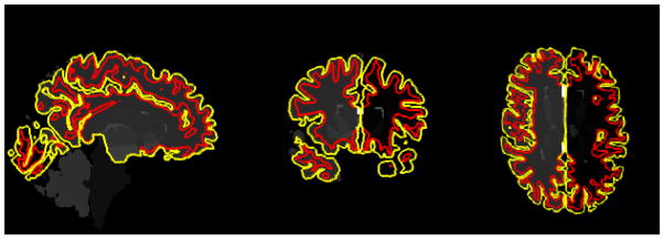
Cortical thickness estimation in magnetic resonance imaging (MRI) is an important technique for Alzheimer’s disease (AD) research. It helps precisely measure the whole-brain and temporal lobe volume atrophy, which has been proven to correlate closely with changes in cognitive performance and is therefore a valid imaging biomarker of AD progression [1]. A number of research has been focused on accurate estimation of cortical thickness (as reviewed in [2]). Currently, two different computational paradigms exist, with methods generally classified as either surface-based [3] or voxel-based [4]. A surface-based thickness computation example is shown in Fig. 1. Between them, surface-based cortical thickness is more widely used in AD research.

Fig. 1.

Three sectional views of pial (yellow) and WM surfaces (red) reconstructed by FreeSurfer. The cortical thickness is estimated by the deformation between them.

There has been a growing interest to apply computer-aided diagnostic classification techniques to analyze cortical thickness features and diagnose different stages of AD and especially in preclinical individuals at high risk for AD to facilitate early interventions. Lerch et al. [5] investigated the potential of fully automated measurements of cortical thickness to reproduce the clinical diagnosis in 19 AD and 17 cognitive unimpaired (CU) subjects. The results show regionally variant patterns of discrimination ability, with over 90% accuracy, but the subject amounts are relative small. Cuingnet et al. [6] constructed a classifier at each vertex by using the cortical thickness as a feature vector. Although the vertex-wise data can reflect local deformity of a small region, they are sensitive to noise and registration errors. Cho et al. [7] overcame the difficulties associated with both types of features by adopting the noise-filtered vertex-wise cortical thickness data based on spatial frequency analysis. This improvement led to an improved accuracy in AD classification. In [8], longitudinal cortical thickness changes were measured by 4D (spatial plus temporal) thickness measuring algorithm. Their proposed method can distinguish AD patients from CU at an accuracy of 96.1%. Nevertheless, having a different systematic approach, which focuses on cortical thickness and validated for different group classifications, including early MCI (EMCI) and later MCI (LMCI), to aid in the diagnosis and understanding of AD progression would be highly advantageous to the preclinical AD research.

Based on the cortical thickness features computed by FreeSurfer, this paper proposes a novel machine learning framework for the diagnosis of different stages of AD. The main contributions of this work are as follows. First, to the best of our knowledge, it is the first sparse coding work formulated on the sphere domain although sparse coding has achieved great success on standard Euclidean image domains [9] and recently in the hyperbolic domain [10]. With an efficient Stochastic Coordinate Coding (SCC) [11][12][13], our work generalizes sparse coding algorithms to the sphere domain and enriches our understanding of sparse coding. Since cortical thickness estimation algorithm generates high dimensional features, some feature reduction algorithms are usually applied before classification. Our second contribution is to adopt novel feature reduction scheme, such as sparse coding and max-pooling [14], which improves the efficiency and efficacy of the performance using high-dimensional cortical thickness on a variety of AD diagnosis tasks. In our work, with the Support Vector Machine (SVM) classifier [15], our system achieved an average of 91.5% on six different classification tasks in our relatively large-sized ADNI2 baseline dataset (N = 201).

2. METHODS

2.1. System Pipeline

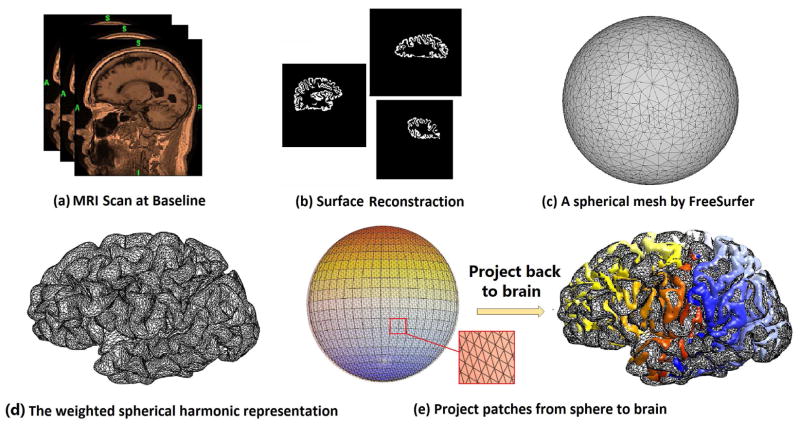
Fig. 2 summarizes the overall pipeline of our new system. FreeSurfer [16] is used to segment images (Fig. 2(a)) and build white matter (WM) and pial cortical surfaces (Fig. 2(b)). FreeSurfer computes the cortical thickness by deforming the WM surface to pial surface and then measuring the deformation distance as the cortical thickness (Fig. 1). FreeSurfer also produces a spherical parameterization for each pial surface (Fig. 2(c)). The spherical parameter surface and weighted spherical harmonics [17] are used to register pial surfaces across subjects (Fig. 2(d)). In our approach, the spherical parameter surface is the canonical space from which patches are selected. Fig. 2(e) shows some non-overlapping patches found on both the spherical surface and the cortical surface. After we compute these patches, sparse coding combined with max-pooling [14] are applied for cortical thickness feature dimension reduction. Max-pooling is an aggregate statistics dimensional reduction technique. It computes the max value of a particular feature over a region of the image. These summary statistics are much lower in dimension than the original data. Finally, SVM classifier is used for classification of different AD clinical groups.

Fig. 2.

Cortical thickness estimation pipeline and spherical patch visualization.

2.2. Weighted Spherical Harmonics for Patch Selection

To build spherical patches on the parameter domain, we need regular underlying grids. However, the spherical parameterization results computed by FreeSurfer do not have regular structures. To overcome this problem, we adopted the weighted spherical harmonic representation (WSHR) [17] to generate the regular grids using the spherical parameterization computed by FreeSurfer. Additionally, the WSHR fixes the Gibbs phenomenon (ringing effects) associated with the traditional Fourier descriptors and spherical harmonic representation by weighting the series expansion with exponential weights. The exponential weights make the representation converges faster and reduces the amount of wiggling. It helps create consistent patches across subjects.

Within the unit sphere parameter space, the mesh parameter coordinates can be represented by the Euler angles θ ∈ [0, π] and φ ∈ [0, 2π) as p(θ, φ) = (p₁(θ, φ); p₂(θ, φ); p₃(θ, φ))′. The weighted spherical harmonic representation of coordinates is then given by

$$p(\theta ,\phi )=\sum _{i=0}^n\sum _{j=-i}^i{e}^{-i(i+1)\mu }{c}_{ij}{s}_{ij}(\theta ,\phi ),$$

where $c_{ij}={\int }_{\theta =0}^{\pi }{\int }_{\phi =0}^{2\pi }p(\theta ,\phi )s_{ij}(\theta ,\phi )sin\theta d\theta d\phi$, and s_ij represents spherical harmonics of degree i and order j. Fig. 2(d) shows an example of the WSHR of 40th degree and set bandwidth μ of zero.

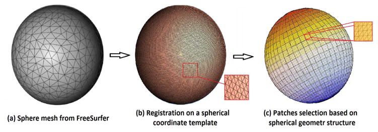
After the cortical hemispheres have been registered with WSHR, consistent patches are defined from the spherical parameter space. As shown in Fig 2e, the spherical coordinate can be projected back to the cortical surface coordinate, which preserves the correspondences between the patches and cortical structures in 3(b). Within the canonical sphere space, it is straightforward to create consistent patches across subjects on spherical coordinates space. The patches are square-shaped on parameter space but distorted on the original surface. They smaller and more distorted at the sphere pole areas. Specifically, a number of 10 × 10 windows (defined by (θ, ϕ)) are created on the sphere to obtain a collection of small image patches based on the spherical geometry structure, shown in Fig. 3(c). The zoomed-in picture shows some overlapping areas between image patches. The procedure is equivalent to applying a high-pass filter to the original mesh. As a result, the geometric structures are still preserved in the centered mesh, but some low frequencies have disappeared.

Fig. 3.

Visualization of computed image patches on spherical geometry structure.

2.3. Sparse Coding and Dictionary Learning

Sparse coding and dictionary learning has been successful in many image processing tasks as it can concisely model natural image patches. In this work, Stochastic Coordinate Coding (SCC) [11] was adopted to construct the dictionary because of its computation efficiency.

Given a finite training set of signals, in this case thickness features, X = (x₁, x₂, ··· , x_n) in R^p×n image patches. Each image patch x_i ∈ R^p, i = 1, 2, · , n, where p is the dimension of image patch and n the number of image patches, the idea of sparse patch features can be incorporated into the following optimization problem:

$$min{f}_i(D,z_i)=\frac{1}{2}{\Vert D{z}_i-x_i\Vert }_2^2+\lambda {\Vert z_i\Vert }_1,$$ (1)

where λ is the regularization parameter, || · || is the standard Euclidean norm and ||z_i||₁ is the summation of all the absolute value of elements from z_i. x_i can be represented by x_i ≈ Dz_i. In this way, the p-dimensional vector x_i is represented by an m-dimensional vector z_i, which means the learned feature vector z_i is a sparse vector of dimension m. In other words, m is the number of sparse codes. The first term of Eq. 1 measures the degree of goodness representing the image patches. The second term ensures the sparsity of the learned feature z_i. D = (d₁, d₂, ··· , d_m) ∈ R^p×m is the dictionary. To prevent an arbitrary scaling of sparse codes, the columns d_j are constrained by

$$C\triangleq \{D\in {\mathbf{R}}^{p\times m}s.t.\forall j=1,\cdots ,m,d_j^T{d}_j\le 1\}.$$

Algorithm 1.

Stochastic Coordinate Coding (SCC) Algorithm

Input: Initial dictionary D and image patches {x1, ··· , xn}.
Output: The learned dictionary and coefficients D, Z where Z = {z1, ··· , zn}.
1:	for t = 1 to T do
2:	for i = 1 to n do
3:	Get an image patch xi
4:	Calculate the sparse code zi by using several steps of coordinate descent (CD) [11]. zi,t+1 = CD(Dt, zi,t, xi)
5:	Update the dictionary D by performing on step stochastic gradient descent (SGD) [11]. Dt+1 = SGD(Dt, zi,t+1)
6:	end for
7:	end for

Thus, the problem of dictionary learning can be rewritten as a matrix factorization problem as follows:

$$\underset{D\in C,\mathbf{Z}\in m\times n}{min}\frac{1}{2}{\Vert X-D\mathbf{Z}\Vert }_F^2+\lambda {\Vert \mathbf{Z}\Vert }_1.$$ (2)

where ${\Vert ·\Vert }_F^2$ is the Frobenius norm. The matrix factorization is a convex problem when either D or Z is fixed. With the initial dictionary D by selected patches, we summarize the SCC algorithm in Algorithm 1. We call each cycle, i.e. each image patch has been trained once, as an epoch. Usually, several epochs are required to obtain a satisfactory result. T is the designed epoch number and t ∈ {1, ..., T}. z_i,t and D_t denotes the value of z_i and D in the t^th epoch. Specifically, we use 7 epochs to learn the dictionary in this work. We set all the sparse codes to be zero at the beginning.

3. EXPERIMENTAL RESULTS

3.1. Datesets and Experiment Setting

In our experiments, the new approach is applied to Alzheimer’s Disease Neuroimaging Initiative (ADNI) 2 database [18]. We used the full set of ADNI2 baseline dataset (202 subjects, 1 failed with FreeSurfer 5.3.0), which consists of: 40 patients of AD, 37 patients of LMCI, 73 patients of EMCI and 51 subjects of CU. All subjects underwent thorough clinical and cognitive assessment at the time of acquisition, the statistics with gender, age and the MiniMental State Examination (MMSE) score shown in Table. 1.

Table 1.

Demographic information of studied subjects in ADNI2 baseline dataset.

Group	Num	F/M	Age	MMSE
AD	40	15/25	75.67±8.87	24.41±4.29
LMCI	37	14/13	73.35±5.91	25.79±2.67
EMCI	73	27/46	72.84±8.14	27.78±2.25
CTL	51	28/23	72.42±6.12	28.64±1.38

3.2. Classification Results

After we applied SCC to learn the sparse features, max-pooling [14] and SVM [15] were applied for additional dimension reduction and classification. We evaluated our proposed method on six classification experiments, including (1) AD vs. CU, (2) AD vs. LMCI, (3) AD vs. EMCI, (4) LMCI vs. CU, (5) EMCI vs. CU and (6) LMCI vs. EMCI. We randomly split the data into training and testing sets using a ratio 6:4 and a 5-fold leave-one-out cross validation protocol was adopted to estimate the classification accuracy. We rotated this procedure for 20 times to estimate the accuracy. In each set of experiment, we compared cortical thickness on left, right hemisphere and both hemispheres (whole brain), respectively. For the comparison purpose, the raw cortical thickness data from FreeSurfer, whole brain volume and area calculated by FreeSurfer were also used as features with SVM as the classifier on the same set of classification tasks.

Three performance measures: Accuracy (ACC), Sensitivity (SEN) and Specificity (SPE) were computed as evaluation [19]. Besides them, we also computed the area-under-the-curve (AUC) of the receiver operating characteristic (ROC) [19]. Table 2 shows classification performance on six different experiments. In our experimental results (Table 2), we can observe that the proposed method always achieved the best results in all six different classification tasks. Specifically, in AD vs. CU, AD vs. LMCI, AD vs. EMCI, LMCI vs. CU, EMCI vs. CU and EMCI vs. LMCI, the best accuracy rates (0.958, 0.933, 0.931, 0.940, 0.884, 0.843) were achieved by our new proposed method using the whole cortical thickness features. And among all six experiments, the new method with whole cortical thickness at least achieved three best measures among all comparisons. And the left thickness feature performs better than right one and always achieved highest sensitivity. Comparing with the Freesurfer thickness results, we observe our method selected useful features which can improve the classification accuracy.

Table 2.

Classification results of six groups of experiments. ThicknessSC is for sparse coding thickness system and FS is for thickness feature of freesurfer with SVM classifier.

Group		ThicknessSC			FS	Vol.	Area
		L	R	W
	ACC	0.90	0.63	0.96	0.62	0.54	0.59
AD	SEN	1.00	1.00	0.91	0.86	0.44	1.00
CU	SPE	0.85	0.60	1.00	0.59	0.57	0.58
	ACC	0.88	0.57	0.93	0.67	0.53	0.65
AD	SEN	0.82	1.00	0.89	0.63	0.51	0.61
LMCI	SPE	1.00	0.52	1.00	0.79	0.58	0.70
	ACC	0.83	0.67	0.93	0.61	0.63	0.62
AD	SEN	1.00	1.00	1.00	0.50	0.68	0.47
EMCI	SPE	0.78	0.65	0.90	0.67	0.36	0.70
	ACC	0.91	0.60	0.94	0.54	0.60	0.46
LMCI	SEN	0.81	1.00	1.00	0.45	0.50	0.32
CU	SPE	1.00	0.60	0.91	0.59	0.61	0.52
	ACC	0.85	0.69	0.88	0.58	0.47	0.50
EMCI	SEN	0.79	0.64	0.82	0.82	0.57	0.52
CU	SPE	1.00	1.00	1.00	0.53	0.38	0.41
	ACC	0.83	0.75	0.84	0.66	0.74	0.69
EMCI	SEN	1.00	1.00	0.81	0.56	0.75	0.50
LMCI	SPE	0.79	0.73	1.00	0.67	0.74	0.69

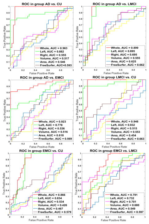
To further compare performance, we also plot ROC curves with computed AUC measures, which are shown in Figure 3. We can find that our new approach always achieved the best AUC among six different testing datasets. For AD vs. CU, AD vs. LMCI, AD vs. EMCI, LMCI vs. CU, EMCI vs. CU and LMCI vs. EMCI, the proposed method achieved the best AUC 0.963, 0.899, 0.923, 0.948, 0.866 and 0.791, respectively. These results show that our new method achieve higher AUC. It means the probability that the classifier will rank a randomly chosen positive example is higher than a randomly chosen negative example and indicates that we may have learned a good classifier.

4. CONCLUSIONS

In this paper, we presented a spherical sparse coding framework, applied it to study cortical thickness feature reduction problem, and evaluated our method on the ADNI2 dataset to check its classification performance. The empirical results, in a total of six comparisons, demonstrated that the spherical sparse coding method achieved greater statistical power than some other standard features.

Fig. 4.

Classification performance comparison with receiver operating characteristic (ROC) curves and area under curve (AUC) measures. Each figure shows results from Whole cortical thickness, left cortical thickness, right cortical thickness, cortical volume and area statistic, respectively.

References

- 1.Frisoni Giovanni B, Fox Nick C, Jack Clifford R, Scheltens Philip, Thompson Paul M. The clinical use of structural MRI in Alzheimer disease. Nature Reviews Neurology. 2010;6(2):67–77. doi: 10.1038/nrneurol.2009.215. [DOI] [PMC free article] [PubMed] [Google Scholar]
- 2.Clarkson Matthew J, Jorge Cardoso M, Ridgway Gerard R, Modat Marc, Leung Kelvin K, Rohrer Jonathan D, Fox Nick C, Ourselin Sébastien. A comparison of voxel and surface based cortical thickness estimation methods. Neuroimage. 2011;57(3):856–865. doi: 10.1016/j.neuroimage.2011.05.053. [DOI] [PubMed] [Google Scholar]
- 3.Fischl Bruce, Dale Anders M. Measuring the thickness of the human cerebral cortex from magnetic resonance images. Proc Natl Acad Sci USA. 2000 Sep;97(20):11050–11055. doi: 10.1073/pnas.200033797. [DOI] [PMC free article] [PubMed] [Google Scholar]
- 4.Jones Stephen E, Buchbinder Bradley R, Aharon Itzhak. Three-dimensional mapping of cortical thickness using Laplace’s equation. Human brain mapping. 2000;11(1):12–32. doi: 10.1002/1097-0193(200009)11:1<12::AID-HBM20>3.0.CO;2-K. [DOI] [PMC free article] [PubMed] [Google Scholar]
- 5.Lerch Jason P, Pruessner Jens, Zijdenbos Alex P, Louis Collins D, Teipel Stefan J, Hampel Harald, Evans Alan C. Automated cortical thickness measurements from MRI can accurately separate Alzheimer’s patients from normal elderly controls. Neurobiology of aging. 2008;29(1):23–30. doi: 10.1016/j.neurobiolaging.2006.09.013. [DOI] [PubMed] [Google Scholar]
- 6.Cuingnet Rémi, et al. Automatic classification of patients with Alzheimer’s disease from structural MRI: a comparison of ten methods using the ADNI database. neuroimage. 2011;56(2):766–781. doi: 10.1016/j.neuroimage.2010.06.013. [DOI] [PubMed] [Google Scholar]
- 7.Cho Youngsang, Seong Joon-Kyung, Jeong Yong, Shin Sung Yong. Individual subject classification for Alzheimer’s disease based on incremental learning using a spatial frequency representation of cortical thickness data. Neuroimage. 2012;59(3):2217–2230. doi: 10.1016/j.neuroimage.2011.09.085. [DOI] [PMC free article] [PubMed] [Google Scholar]
- 8.Li Yang, Wang Yaping, Wu Guorong, Shi Feng, Zhou Luping, Lin Weili, Shen Dinggang. Discriminant analysis of longitudinal cortical thickness changes in Alzheimer’s disease using dynamic and network features. Neurobiology of aging. 2012;33(2):427–e15. doi: 10.1016/j.neurobiolaging.2010.11.008. [DOI] [PMC free article] [PubMed] [Google Scholar]
- 9.Mairal Julien, Bach Francis, Ponce Jean, Sapiro Guillermo. Online dictionary learning for sparse coding. Proceedings of the 26th annual international conference on machine learning; ACM; 2009. pp. 689–696. [Google Scholar]
- 10.Zhang Jie, Shi Jie, Stonnington Cynthia, Li Qingyang, Gutman Boris A, Chen Kewei, Reiman Eric M, Caselli Richard, Thompson Paul M, Ye Jieping, Wang Yalin. International Conference on Medical Image Computing and Computer-Assisted Intervention. Springer; 2016. Hyperbolic space sparse coding with its application on prediction of Alzheimers disease in mild cognitive impairment; pp. 326–334. [DOI] [PMC free article] [PubMed] [Google Scholar]
- 11.Lin Binbin, Li Qingyang, Sun Qian, Lai Ming-Jun, Davidson Ian, Fan Wei, Ye Jieping. Stochastic coordinate coding and its application for drosophila gene expression pattern annotation. 2014 arXiv preprint arXiv:1407.8147. [Google Scholar]
- 12.Zhang Jie, Stonnington Cynthia, Li Qingyang, Shi Jie, Bauer Robert J, Gutman Boris A, Chen Kewei, Reiman Eric M, Thompson Paul M, Ye Jieping, Wang Yalin. Applying sparse coding to surface multivariate tensor-based morphometry to predict future cognitive decline. Biomedical Imaging (ISBI), 2016 IEEE 13th International Symposium on; IEEE; 2016. pp. 646–650. [DOI] [PMC free article] [PubMed] [Google Scholar]
- 13.Zhang Jie, Wang Yalin, et al. Patch-based sparse coding and multivariate surface morphometry for predicting amnestic mild cognitive impairment and alzheimers disease in cognitively unimpaired individuals. Alzheimer’s & Dementia: The Journal of the Alzheimer’s Association. 2016;12(7):P947. [Google Scholar]
- 14.Scherer Dominik, Müller Andreas, Behnke Sven. Artificial Neural Networks–ICANN 2010. Springer; 2010. Evaluation of pooling operations in convolutional architectures for object recognition; pp. 92–101. [Google Scholar]
- 15.Boser Bernhard E, Guyon Isabelle M, Vapnik Vladimir N. A training algorithm for optimal margin classifiers. Proceedings of the fifth annual workshop on Computational learning theory; ACM; 1992. pp. 144–152. [Google Scholar]
- 16.Fischl Bruce. Freesurfer. Neuroimage. 2012;62(2):774–781. doi: 10.1016/j.neuroimage.2012.01.021. [DOI] [PMC free article] [PubMed] [Google Scholar]
- 17.Chung Moo K, Dalton Kim M, Shen Li, Evans Alan C, Davidson Richard J. Weighted fourier series representation and its application to quantifying the amount of gray matter. Medical Imaging IEEE Transactions on. 2007;26(4):566–581. doi: 10.1109/TMI.2007.892519. [DOI] [PubMed] [Google Scholar]
- 18.Wyman Bradley T, Harvey Danielle J, et al. Standardization of analysis sets for reporting results from ADNI MRI data. Alzheimer’s & Dementia. 2013;9(3):332–337. doi: 10.1016/j.jalz.2012.06.004. [DOI] [PMC free article] [PubMed] [Google Scholar]
- 19.Fawcett Tom. An introduction to ROC analysis. Pattern recognition letters. 2006;27(8):861–874. [Google Scholar]