Improving the magnetoelectric performance of Metglas/PZT laminates by annealing in a magnetic field

Abstract

A comprehensive investigation of magnetostriction optimization in Metglas 2605SA1 ribbons is performed to enhance magnetoelectric performance. We explore a range of annealing conditions to relieve remnant stress and align the magnetic domains in the Metglas, while minimizing unwanted crystallization. The magnetostriction coefficient, magnetoelectric coefficient, and magnetic domain alignment are correlated to optimize magnetoelectric performance. We report on direct magnetostriction observed by in-plane Doppler vibrometer and domain imagining using scanning electron microscopy with polarization analysis for a range of annealing conditions. We find that annealing in an oxygen-free environment at 400 °C for 30 min yields an optimal magnetoelectric coefficient, magnetostriction and magnetostriction coefficient. The optimized ribbons had a magnetostriction of 50.6 ± 0.2 μm m⁻¹ and magnetoelectric coefficient of 79.3 ± 1.5 μm m⁻¹ mT⁻¹. The optimized Metglas 2605SA1 ribbons and PZT-5A (d₃₁ mode) sensor achieves a magnetic noise floor of approximately 600 pT Hz^−1/2 at 100 Hz and a magnetoelectric coefficient of 6.1 ± 0.03 MV m⁻¹ T⁻¹.

1. Introduction

The magnetoelectric (ME) effect is the coupling of the magnetostrictive and the piezoelectric phenomena. In multi-layered laminate structures, magnetic sensing is achieved by transduction of the magnetostrictive effect, where a strain induced by a magnetic field is elastically coupled to the piezoelectric layer and in turn produces a charge. The electrically induced magnetoelectric effect was first demonstrated in Cr₂O₃ by Astrov [1] and shortly after the magnetically induced variety was observed by Rado and Folen [2]. Philips Laboratories demonstrated that composites can greatly enhance the magnetoelectric effect over single-phase material, achieving a magnetoelectric coefficient of 0.13 MV m⁻¹ T⁻¹ [3–5]. The magnetoelectric coefficient is commonly presented in CGS system of units of V cm⁻¹ Oe⁻¹. In this work, we use the MKS system of units equivalent of MV m⁻¹ T⁻¹ which results in the same numerical value as the conventional CGS units assuming the test is done in a medium of relative permeability, μ_r, very close to 1 (i.e., 1 V cm⁻¹ Oe⁻¹ (μ₀μ_r)⁻¹ = 1 MV m⁻¹ T⁻¹ for μ_r = 1, where μ₀ is the permeability of free space). The strongest ME effects occur in laminates composed of materials exhibiting strong magnetostriction without piezoelectricity elastically coupled to materials with strong piezoelectricity without magnetostriction; this allows the two crucial phenomena to be separately optimized [6, 7]. In this work we optimize the magnetostrictive component through a comprehensive analysis of the magnetostriction coefficient, domain imaging and magnetoelectric coefficient.

Understanding and optimizing the magnetoelectric coefficient is of great interest to the biomagnetic community as a magnetometer [8], remote actuator [9], and implantable pressure sensor [10]. Inexpensive room temperature magnetometers capable of biomagnetic measurements have the potential to replace costlier superconducting quantum interference devices and increase patient access. Extensive work is also being done on ME devices for energy harvesting [11, 12]. The soft magnetic properties of magnetostrictive amorphous alloys, like Fe–Si–B [13], have been used in the development of highly sensitive room temperature magnetic sensors. Magnetoelectric coefficients of up to 52 MV m⁻¹ T⁻¹ and 3 pT Hz^−1/2 at 1 Hz sensitivity for laminates of Metglas⁵ and (1 − x)[Pb(Mg_1/3Nb_2/3)O₃]−x[PbTiO₃] (PMN-PT) have been reported [14, 15].

It has been generally established that annealing in the presence of a magnetic field induces an anisotropy and increases magnetostriction in amorphous metallic glasses. Several groups have explored the effect of annealing amorphous metallic glasses on the elastic modulus (ΔE effect) [16–20], magnetostriction [19–22], and embrittlement [23]. Annealing optimization has been applied in a limited fashion for magnetoelectric devices [24]. This is because despite the plethora of work in this field, the effects of annealing on ME device performance from one material formulation of amorphous metal does not necessarily translate to other material formulations (some Metglas formulations near-zero magnetostriction [25]) and, to complicate the matter, the manufacturing of the amorphous metal foils is critical to their performance and varies between suppliers. There is no comprehensive work on a single material that provides clear guidance on how to optimize a Metglas 2605SA1 magnetoelectric device. Furthermore, most work focuses on optimizing the saturation magnetostriction; however it is the magnetostriction coefficient (peak of the slope of the magnetostriction versus applied magnetic field) which is the crucial figure of merit for a magnetostrictive ribbon in a magnetoelectric device.

To address these deficiencies we have calculated the magnetostriction coefficient from magnetostriction measurements under a variety of annealing conditions. In order to create a comprehensive guide for optimization of Metglas 2605SA1/PZT (Pb[Zr_xTi_1−x]O₃) ME sensors through field annealing we consider four main factors: (1) temperature (2) time (3) applied transverse magnetic field (4) oxygen in the ambient environment. We also correlate these results the with magnetoelectric coefficient measured on Metglas 2605SA1 and PZT-5A laminates in d₃₁ sensing mode. Furthermore, we have performed scanning electron microscopy with polarization analysis (SEMPA) to observe the domain alignment.

2. Theory

Aligning the easy axis of a magnetostrictive film ensures that the domains produce the largest amount of magnetostriction (λ) in response to a magnetic field perpendicular to the easy axis. The illustration in figure 1(a) shows randomly oriented magnetic domains in a magnetostrictive film after application of a saturation magnetic field to have a strain of λ_s. For a film where the domains are forced to rotate 90° in response to an applied saturation magnetic field, the maximum strain of λ_max is produced, as seen in figure 1(b). The difference between the random and perpendicular alignment can be understood by (1), where θ_i and θ_f are the initial and final magnetization angles relative to the applied magnetic field [26].

$${\lambda }_{max}=\frac{3}{2}{\lambda }_s({\cos }^2{\theta }_{\mathrm{f}}-{\cos }^2{\theta }_{\mathrm{i}}).$$ (1)

Figure 1.

Illustration showing magnetic domains initially in (a) a random orientation and (b) perpendicular orientation before and after magnetic alignment, respectively. With random domain alignment, a strain of λ_s is possible. When the domains are aligned perpendicular to the applied magnetic field, B, a maximum amount of strain (λ_max) can be achieved.

λ_s is the saturation magnetostriction for isotropically (randomly) distributed magnetic domains. Assuming the easy axis is perfectly perpendicular to the applied field, (i.e., θ_i = π/2 and θ_f = 0), then ${\lambda }_{max}=\frac{3}{2}{\lambda }_{\mathrm{s}}$; a maximum 2 improvement of 50% in the magnetostriction is possible. The magnetoelectric coefficient (α_me) is defined in (2), where V is the measured voltage, B is the applied magnetic field and t is the electrode spacing on the piezoelectric. The magnetoelectric coefficient is equivalent to the product of the piezoelectric voltage coefficient $\left(\frac{\partial E}{\partial S}\right)$ and the magnetostrictive coefficient $\left(\frac{\partial \lambda }{\partial B}\right)$ as seen in (2), where E is the electric field and S is the strain.

$${\alpha }_{\text{me}}=\frac{\mathrm{\Delta }V}{t\mathrm{\Delta }B}=\frac{\partial E}{\partial S}\frac{\partial \lambda }{\partial B}.$$ (2)

Metglas 2605SA1 has a relatively small λ_s of 27 μm m⁻¹ [27] when compared to Terfenol-D and Fe–Ga based alloys, which show a λ_s of 2400 μm m⁻¹ [28] and 325 μm m⁻¹ [29], respectively. While a large λ_s is preferable for actuation, sensing applications require a high magnetostrictive coefficient. Metglas 2605SA1 has among the highest reported with $\left(\frac{\partial \lambda }{\partial H}\right)=36\mathit{\mu }\mathrm{m}{\mathrm{m}}^{-1}{\text{mT}}^{-1}$ for thin films [30], compared to 12 μm m⁻¹ mT⁻¹ for Terfenol-D [31]. An increased magnetostriction coefficient results in a larger Δλ for a given ΔB and thus the α_me will be improved. Further improvements are likely by removing internal stresses which can act as magnetic domain pinning centers preventing the domains from rotating in unison.

3. Methods

3.1. Metglas annealing

The 5 ± 0.5 mm × 30 ± 0.5 mm, 23 μm thick Metglas 2605SA1 ribbons are annealed on a custom built hotplate. The hotplate is built from non-ferromagnetic components to minimize unwanted magnetic fields during the anneals. The heater is an alumina metallic ceramic heating element held between two aluminum plates to ensure uniform heat distribution. Metglas 2605SA1 ribbons are cut and clamped onto the aluminum plates of the hotplate using a silicon piece and held down with aluminum clips. The cutting of the ribbons is done prior to annealing because Fe–Si–B amorphous alloys like Metglas 2605SA1 can undergo embrittlement from heat treatments, making it difficult to cut after annealing. A K-type thermocouple is also inserted between an aluminum clip and the silicon to monitor the temperature. A pair of SmCo high temperature magnets are placed approximately 25 mm apart, with the North–South poles facing each other on a glass fixture and secured with copper tape to provide a magnetization field along the short axis of the ribbons. The heater and magnets are placed on a thermally insulating ceramic slab. An air gap between the aluminum plates and the magnets ensures that the magnets do not exceed their maximum operating temperature of 300 °C. The Metglas placed in the center of the heater experiences approximately 160 ± 20 mT, determined by a calibrated commercial magnetometer. The uncertainty in the magnetic field strength is due to the spatial variation of the magnetic field over the annealing area, again determined by a calibrated commercial magnetometer. The ribbons are allowed to cool until they reach 80 °C or lower before they are removed from the annealing setup and used in the fabrication of a magnetoelectric device, for SEMPA imaging, or for measuring magnetostriction.

3.2. Magnetostriction

After annealing the Metglas ribbons are clamped at one end and the strain on the free edge is measured. The magnetostriction is measured using a 3D laser Doppler vibrometer at the tip of the free end of the Metglas ribbon. A benefit of this method is that it eliminates the influence of a contact transducer like a strain gauge. Also, this system is capable of directly measuring in-plane motion so a unimorph structure is not required. A pair of Helmholtz coils, calibrated with a commercial magnetometer, are used to apply the magnetic field in a controlled manner. The measurement is repeated 4 times and smoothed to remove high frequency noise. The uncertainty of the saturation magnetostriction is reported as ±1σ (one standard deviation) determined from the repeats. A derivative with respect to the applied magnetic field is performed to plot the magnetostrictive coefficient. The magnetostriction coefficients reported in the text of the article refer to the peak value. The uncertainty in magnetostriction coefficient is reported as ±1σ (one standard deviation) from values calculated from the repeats.

3.3. SEMPA imaging

We use SEMPA [32, 33] to image the magnetic domain structure of the Metglas ribbons at the surface and quantitatively assess the alignment of the domains induced by annealing. SEMPA is a scanning electron microscopy technique which images all three components of the magnetization vector of a ferromagnetic sample by determining the polarization direction of the secondary electrons for each pixel of a scan. Metglas samples measuring 5 ± 0.5 mm × 15 ± 0.5 mm are used for this experiment. After annealing, the ribbons are cleaned in situ with 1000 eV Ar ion etching immediately prior to SEMPA imaging. Five 254 μm × 254 μm SEMPA images of different regions are taken for each annealing condition in order to accurately determine the typical domain structure produced by each anneal. Only the shiny side (the rough side is the face in contact with the roller during the quenching process) of the Metglas ribbon is imaged.

3.4. Magnetic sensing

To measure the magnetoelectric coefficient, laminate structures are fabricated using 3 mm × 13 mm × 200 thick μm PZT-5A and a pair of 5 ± 0.5 mm × 30 ± 0.5 mm, 23 μm thick Metglas 2605SA1 ribbons. The PZT has 15 μm thick silver on the top and bottom deposited by the manufacturer and is electrically poled in the d₃₁ orientation (also by the manufacturer). The final device structure is illustrated in figure 2. First, a pair of Metglas ribbons undergo various annealing treatments, then the ribbons are epoxied using EPO-TEK H20E (see footnote 5) conductive silver epoxy on the top and bottom of the PZT. The laminate is mechanically clamped to ensure a thin and uniform epoxy layer and is cured for at least 180 min at 90 °C. Simulations have shown that an epoxy with a modulus of 5 GPa to 10 GPa applied as thinly as possible is crucial for optimal stress transfer between the laminates [34]. Next, a small 3 mm × 5 mm section of the bottom of the laminate is epoxied to a ceramic holder with a silver electrode trace, and the trace is connected to a copper wire. The top of the laminate is also connected with a copper wire. Both wires are secured by H20E epoxy, and the assembly is cured again for at least 180 min at 90 °C.

Figure 2.

Cross section of the device structure showing the 3 mm × 13 mm, 200 μm thick PZT-5A with 15 μm silver top and bottom electrodes. The 23 μm thick 5 mm × 30 mm Metglas ribbons are epoxied on the top and bottom by a conductive silver epoxy.

The devices are tested in a custom designed box with three layers of magnetic shielding. Two pairs of Helmholtz coils are used for DC and AC magnetic stimulation inside the shielded box (figure 3). An AC current source is used to automatically adjust for impedance variations in the coil and provide a stable magnetic field strength across a range of frequencies. The voltage generated by the PZT is measured by a lock-in amplifier as seen in the illustration of the test setup in figure 3. The peak magnetoelectric voltage coefficient is determined by applying a DC magnetic bias to the ME device in the steepest portion of the magnetostriction curve (peak magnetoelectric coefficient), which is typically 500 μT to 1500 μT, and consistent with observations from other groups [15, 24]. All magnetoelectric coefficient measurements are done with a 20 Hz sine signal at 5.6 μT. For magnetic noise floor measurements, the lock-in amplifier is replaced by a digital spectrum analyzer.

Figure 3.

Diagram of the testing setup. A DC source and an AC current source are used for stimulation. The ME device is directly connected to a lock-in amplifier. For noise measurements, the lock-in is replaced with a digital spectrum analyzer.

4. Results and discussion

To study the impact of temperature on magnetostriction we anneal from 250 °C to 400 °C for 5 min in air. The magnetostriction is measured by laser Doppler vibrometer, shown in figure 4. The magnetostriction coefficient is calculated from the derivative of the magnetostriction, with respect to the magnetic field. Two grouping of curves are observed; Group 1 shows no trend with annealing temperature. Group 2 shows an increase in saturation magnetostriction and magnetostriction coefficient from 16.7 ± 1.6 μm m⁻¹ mT⁻¹ to 21.0 ± 0.7 μm m⁻¹ mT⁻¹. Without an applied field the domains may be susceptible to the influence of internal and/or external stresses.

Figure 4.

Magnetostriction and magnetostriction coefficient (dashed lines) for 5 min anneals without an applied magnetic field in air. Both λ and $\left(\frac{\partial \lambda }{\partial B}\right)$ are difficult to control without an external field present during annealing. Some other variable, possibly stress from the manufacturing process, is causing the samples to split into two groups of magnetostrictive curves.

Next we consider the effect of annealing the samples in a 160 mT transverse magnetic field; we again annealed from 250 °C to 400 °C in air. Figure 5 shows the knee of the magnetostriction curve increases with increasing annealing temperature. As a result, the magnetostriction coefficient increases with increasing annealing temperature from 11.6 ± 0.4 μm m⁻¹ mT⁻¹ for the as-cast sample to 77.5 ± 2.2 μm m⁻¹ mT⁻¹ for the 400 °C 5 min anneal in an applied magnetic field in air.

Figure 5.

Magnetostriction and magnetostriction coefficient (dashed lines) for 5 min anneals with an applied magnetic field in air. The knee of the magnetostriction increases with increasing annealing temperature. The magnetostriction coefficient also increases with increasing annealing temperature.

To confirm the magnetostriction coefficient increase translates into a magnetoelectric coefficient improvement we fabricate and test magnetoelectric devices. Pairs of Metglas ribbons are annealed for 5 min from 250 °C to 450 °C in atmospheric conditions with and without a 160 mT magnetic field. The average peak α_me measured for each annealing condition is shown in figure 6. The average peak α_me is determined by sweeping positive and negative DC magnetic field where the uncertainty represents the entire range of measurements collected for each sample (± half range). The worst case repeatability range is ±0.05 MV m⁻¹ T⁻¹. The resulting error bars are too small to be seen in the plot.

Figure 6.

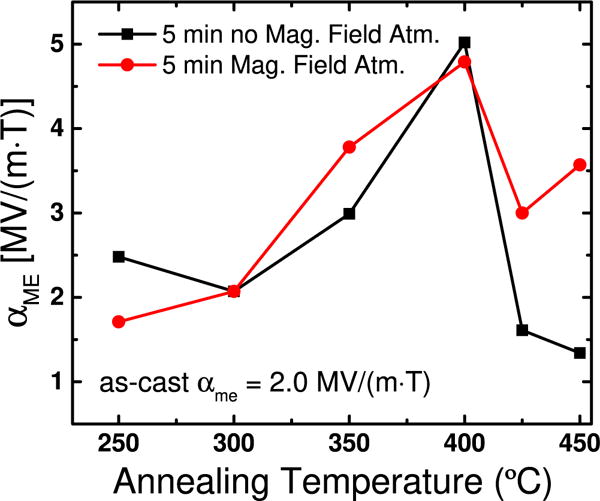
Magnetoelectric coefficient α_me versus annealing temperature for samples annealed with and without an applied magnetic field. Up to 400 °C, the trends of the samples annealed with and without a magnetic field are similar. For both cases the magnetoelectric coefficient increases to approximately 5.0 ± 0.04 MV m⁻¹ T⁻¹. After 400 °C, the α_me decreases for both cases. Lines are added as a guide to the reader. The error bars described in the text are smaller than the point markers. Note that 1 V cm⁻¹ Oe⁻¹ (μ₀μ_r)⁻¹ = 1 MV m⁻¹ T⁻¹ for μ_r = 1.

The magnetoelectric coefficient increases with increasing annealing temperature up to 400 °C. However, the magnitude of improvement from as-cast to 400 °C is lower, 2.5-fold improvement in magnetoelectric coefficient versus 6.7-fold improvement the magnetostriction coefficient. Surprisingly, the magnetoelectric devices fabricated using ribbons without an applied magnetic field during the anneal improved by approximately the same magnitude as samples made with ribbons that were annealed with a magnetic field. This suggests that annealing makes the domains more susceptible to influence from the magnetoelectric fabrication process, possibly from compressive stress applied by the epoxy cure process.

To directly observe the domain alignment we perform SEMPA imaging on Metglas ribbons annealed for 5 min from 250 °C to 400 °C in air with and without a magnetizing field. Figures 7(a)–(e) shows the typical magnetic domains observed for Metglas strips in the as-cast state (a) and after 250 °C to 400 °C, 5 min annealing in a magnetic field along the x-axis (b)–(e). The histogram plot adjacent to each image shows the distribution of domain direction after mirroring about the y-axis. Figures 7(a)–(c) shows that stress-induced striations are visible for the as-cast sample and for samples annealed up to 300 °C. These occur because out-of-plane magnetic domains induced by stress must rotate to in-plane domains at the surface and curl back into the sample [35]. At 350 °C and higher, the area of observed stress-induced striations is significantly reduced, which implies a reduction in out-of-plane domains, and correlates to an increase in the α_me.

Figure 7.

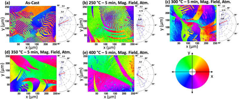
Typical 254 μm × 254 μm SEMPA images and angle histograms of as-cast samples (a), and samples annealed for 5 min in a 160 mT magnetic field. The magnetization direction is coded to the color wheel, with red indicating magnetization pointing in the +x direction, green indicating magnetization pointing in the +y direction, etc. Stress-induced striations are visible in as-cast, 250 °C and 300 °C annealed samples. For samples annealed at 350 °C and 400 °C the striations are rarely observed. The red bar in the polar histograms points to the average magnetization direction. There is no evidence of an induced easy-axis alignment. The angle distribution is not ideal for maximum magnetostriction.

Despite the dramatic improvement in saturation magnetostriction, magnetostriction coefficient, and magnetoelectric coefficient observed in figures 5 and 6, the SEMPA images, seen in figures 7(b)–(e), show the magnetic ordering did not align along the magnetizing field axis for any annealing condition. The magnetization of the Metglas ribbons annealed without the magnetizing field (not shown) had similar characteristics and did not show easy axis alignment. SEMPA is a surface imaging technique and can not capture alignment that is occurring in the bulk of the ribbon. The increase in saturation magnetostriction and magnetostriction coefficient when annealing in an applied magnetic field implies that the domains are aligning, and the lack of domain alignments observed by SEMPA suggests that further optimization may be possible.

To optimize the magnetostriction coefficient and the magnetoelectric coefficient, by inducing further transverse magnetic alignment in the Metglas ribbons, we increase the duration of anneals. Magnetostriction data is collected for Metglas ribbons annealed between 350 °C and 450 °C for 30 min in various environments in an applied magnetic field. We removed oxygen from the annealing environment to prevent oxidation of the Metglas by annealing in a vacuum chamber which is triple pump-purged with nitrogen and pumped to 1.33 × 10⁴ Pa (100 Torr) or by annealing in a continuous N₂ purge. Figure 8 shows the that for every annealing temperature a higher saturation magnetostriction and magnetostriction coefficient are observed for anneals done in an oxygen-free environment. The highest saturation magnetostriction of 50.6 ± 0.2 μm m⁻¹ and magnetoelectric coefficient of 79.3 ± 1.5 μm m⁻¹ mT⁻¹, respectively, were measured for the 400 °C 30 min anneal with an applied magnetic field in an N₂ environment. The saturation magnetostriction and magnetoelectric coefficient decrease significantly for the 30 min 450 °C anneals and are exceptionally poor for the sample annealed in atmosphere.

Figure 8.

Magnetostriction and magnetostriction coefficient (dashed lines) for 30 min anneals with an applied magnetic field in varying environments. Both λ and $\left(\frac{\partial \lambda }{\partial B}\right)$ increase for anneals done in an oxygen-free environment for the same temperature. Optimal Both λ and $\left(\frac{\partial \lambda }{\partial B}\right)$ is found to be 50.6 ± 0.2 μm m⁻¹ and magnetoelectric coefficient of 79.3 ± 1.5 μm m⁻¹ mT⁻¹, respectively, for the 400 °C 30 min anneal with an applied magnetic field in an N₂ environment.

Increasing the anneal time from 5 min to 30 min at 350 °C in air results in a linear decrease of the magnetoelectric coefficient from 3.8 ± 0.04 MV m⁻¹ T⁻¹ to 2.0 ± 0.03 MV m⁻¹ T⁻¹, as seen in figure 9. Similarly, figure 9 shows the α_me decreases from 5.0 ± 0.04 to 4.1 ± 0.05 MV m⁻¹ T⁻¹ when the anneal time is increased from 5 min to 30 min at 400 °C. The SEMPA image in figure 10(a) shows that a 30 min 350 °C anneal in air does not result in domain alignment on the surface. However, SEMPA images taken after a 30 min 400 °C anneal in air reveal a strong magnetic domain alignment in the x-axes, parallel to the magnetic field applied during the anneal as seen in figure 10(b).

Figure 9.

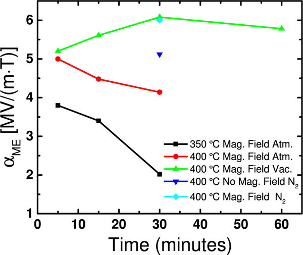
Increasing the anneal time from 5 min to 30 min decreases the magnetoelectric coefficient for 350 °C and 400 °C annealed samples in air with an applied magnetic field. However, annealing in vacuum resulted in a 1.2× improvement for a 400 °C 30 min anneal compared to a 5 min 400 °C anneal in atmosphere with an applied magnetic field. A 60 min 400 °C anneal in vacuum with an applied magnetic field did not result in further improvement, suggesting the magnetic domain alignment had saturated at 30 min. The α_me = 5.0 ± 0.04 MV m⁻¹ T⁻¹ for a sample annealed for 30 min at 400 °C in N₂ without an applied magnetic field is comparable to that measured for samples annealed for 5 min at 400 °C in atmosphere with and without an applied magnetic field. The α_me = 6.1 ± 0.03 MV m⁻¹ T⁻¹ measured for a 30 min 400 °C anneal in N₂ with an applied magnetic field is comparable to the 30 min 400 °C vacuum anneal with an applied magnetic field. This confirms oxygen plays a role in the α_me degradation for anneals longer than 5 min. The error bars are described in the text and are smaller than the point markers. Note that 1 V cm⁻¹ Oe⁻¹ (μ₀μ_r)⁻¹ = 1 MV m⁻¹ T⁻¹ for μ_r = 1.

Figure 10.

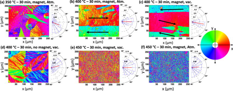
254 μm × 254 μm typical SEMPA images and angle histograms. (a) Annealing at 350 °C with a magnetic field in atmosphere did not result in domain alignment on the surface. Samples annealed for 30 min at 400 °C in a magnetic field applied along the x-axis shows strong easy axis alignment for both the vacuum (b) and atmosphere (c) cases. Arrows are added to indicate to the approximate domain direction. As expected, annealing for 30 min at 400 °C in a vacuum without a magnetic field does not result in magnetic domain alignment (d). Annealing at 450 °C for 30 min in (e) vacuum results in fine magnetic domain structures with a weak alignment, but annealing in (f) air shows no preferred domain alignment axis.

Metglas ribbons are annealed in a vacuum chamber at 400 °C for (5, 15, 30 and 60) min in a magnetic field. The ME device fabricated from samples annealed for 5 min in vacuum, show a magnetoelectric coefficient that is comparable to that produced by the atmosphere anneal case, meaning short anneals are not significantly affected by the atmospheric environment. After 15 min and 30 min of vacuum annealing, the magnetoelectric coefficient increases to 5.6 ± 0.05 MV m⁻¹ T⁻¹ and 6.1 ± 0.04 MV m⁻¹ T⁻¹, respectively. Further annealing for 60 min in vacuum does not result in any significant change in the magnetoelectric coefficient. SEMPA imaging of ribbons annealed for 30 min in vacuum in an applied magnetic field shows easy axis alignment along the magnetic field direction in figure 10(c). To confirm that the domain alignment is in response to the applied magnetic field, SEMPA imaging is performed on a 30 min 400 °C vacuum sample annealed without a magnetic field. Figure 10(d) confirms that the domains do not align without magnetic field present during annealing. SEMPA imaging on 450 °C 30 min anneals in an applied magnetic field reveals a fine magnetic domain structure that is heavily influenced by crystallization on the surface. The 450 °C samples were clearly more polycrystalline when observed under traditional scanning electron microscopy imaging (not shown) compared to the all other samples. Visual inspection of figure 10(e), the SEMPA image taken for the 450 °C 30 min anneal in an applied magnetic in vacuum, does show obvious signs of domain alignment however the histogram shows an alignment in the x-axis with a large Gaussian spread. The SEMPA image and histogram for the 450 °C 30 min anneal in an applied magnetic in air show no preferred alignment.

To quantify the magnetic easy axis alignment, we have developed a figure of merit. We cannot use the average or standard deviation of the domain angle as useful figures of merit. The average can not distinguish between a set of domains that are approximately mirrored about the x-axis and domains that are actually pointing in the x-axis. The standard deviation only describes the variation of the angles and not their direction. To capture both the variation and direction of the domain angle, the standard deviation equation is modified to be the standard deviation (σ₀) around 0° (parallel to the magnetizing field), as shown in (3). N is the number of pixels in each image, ϕ_i is the magnetization direction of each pixel, and ϕ_m is the direction of the desired magnetization direction (0° in this case). A smaller σ₀ value indicates a higher degree of alignment along the x-axis.

$${\sigma }_0=\sqrt{\frac{1}{N}{\displaystyle \sum _{i=1}^N{({\varphi }_i-{\varphi }_{\mathrm{m}})}^2}}.$$ (3)

Table 1 shows the average σ₀ for each annealing condition imaged by SEMPA. The ribbons showing the best qualitative domain alignment in figure 10 also showed the best quantitative alignment by having the lowest σ₀. The ribbons annealed in an applied magnetic field at 400 °C for 30 min in atmosphere and vacuum have a σ₀ = 37.9° and 42.2°, respectively. This is lower than the σ₀ determined for samples that did not show strong magnetic domain alignment, which were between 48.9° and 62.8°. Two notable exceptions were the as-cast, and 350 °C 5 min atmospheric zero-field-anneal samples. In the as-cast case, manufacturing induced stress may have contributed to a preferred domain direction. Also, it should be noted that SEMPA does not provide detailed information about the bulk domains magnetized out-of-plane, but we observe evidence of closure domains in the as-cast sample. For the 350 °C, 5 min atmospheric zero-field-annealed case, one possible explanation is that the large domains that form at higher annealing temperatures make it more difficult to get a good representation of the domain variation in the sample within the field of view of the SEMPA images, resulting in a higher chance of observing outliers. It should also be noted that while the σ₀ appears to be high for aligned samples, it is not unexpected as significant moment canting has been observed in Fe–Si–B amorphous metallic glass with standard deviations of moment spread of 12° reported for an applied field of 0.5 T [36].

Table 1.

σ₀ for every set of SEMPA images. The lowest σ₀ achieved from samples annealed for 30 min at 400 °C in an applied magnetic field in either vacuum or atmosphere. The as-cast sample σ₀ of 39.0° is low, possibly due to stress-induced alignment. The uncertainty is calculated as ±1σ (one standard deviation) of the σ₀ calculated from the set of five images collected for each annealing condition.

Anneal temp. (°C)	Time (min)	Field (mT)	Environment	σ0 (°)
As-cast	N/A	N/A	N/A	39.0 ± 15.7
250	5	0	Atm.	52.3 ± 5.6
300	5	0	Atm.	52.2 ± 7.5
350	5	0	Atm.	41.9 ± 4.3
400	5	0	Atm.	51.5 ± 7.0
250	5	160	Atm.	62.8 ± 5.7
300	5	160	Atm.	57.4 ± 7.4
350	5	160	Atm.	55.7 ± 9.0
400	5	160	Atm.	57.3 ± 12.3
350	30	160	Atm.	48.9 ± 8.4
400	30	160	Atm.	37.9 ± 5.7
400	30	160	Vac.	42.2 ± 4.8
400	30	0	Vac.	51.5 ± 3.1
450	30	160	Vac.	46.5 ± 1.0
450	30	160	Atm.	51.6 ± 0.3

We investigate the extent of oxidation in the Metglas. a thickness profile is conducted by x-ray photoelectron spectroscopy (XPS) on a series of samples annealed for 30 and 60 min in N₂, vacuum, and atmosphere at 400 °C. No other elements besides Fe, Si, B, and O were observed. Figure 11 shows the atomic concentration of oxygen as a function of thickness. The oxide thickness, shown in table 2, is taken to be the depth at which the O concentration falls to half its original value and has an uncertainty of ±1 nm due to finite step size of the Ar etching. The samples annealed in atmosphere for 30 min and 60 min had the largest oxide layers of 6.7 nm and 7.6 nm, respectively. The 30 min and 60 min vacuum annealed samples had oxide thicknesses of 4.6 nm and 5.5 nm, respectively. In both cases, longer anneals resulted in a thicker oxide layer. The thinnest oxide (3.3 nm) resulted from a 60 min N₂ anneal and was comparable to the 3.9 nm oxide layer measured for the un-annealed as-cast sample. The oxide thicknesses are very thin compared to the Metglas foil thickness, and it is not clear if the oxide layer is impacting the magnetoelectric coefficient and by what mechanism. One possibility is that the formation of the oxide layer leads to stress and deformation-assisted crystallization which results in nanocrystallites forming, which has been observed in similar Fe–Si–B amorphous ribbons [37, 38]. Oxygen is known to significantly increase the rate of crystallization in this phenomenon [39].

Figure 11.

Thickness profile of oxygen atomic concentration for various 400 °C annealing conditions. Annealing in atmospheric conditions results in thicker oxides compared to vacuum or N₂ anneals. The uncertainty is determined by measuring the percent standard deviation of the boron atomic concentration below the oxide layer (which should be constant) for each sample and applying the percent standard deviation to each data point of oxygen concentration.

Finally, to gauge the performance of the optimized device in real-world sensor applications, the magnetic equivalent noise floor is measured using a digital spectrum analyzer while applying a 25 Hz 5.6 nT test signal to the optimized ME device made from ribbons subjected to a 30 min, 400 °C vacuum anneal in a magnetizing field and an ME device made from as-cast ribbons. Figure 12 shows the equivalent magnetic noise floor of approximately 600 pT Hz^−1/2 at 100 Hz for the optimized device. The as-cast device showed a magnetic noise floor of 1.6 nT Hz^−1/2 at 100 Hz. Noise at 60 Hz and its harmonics are also visible.

Figure 12.

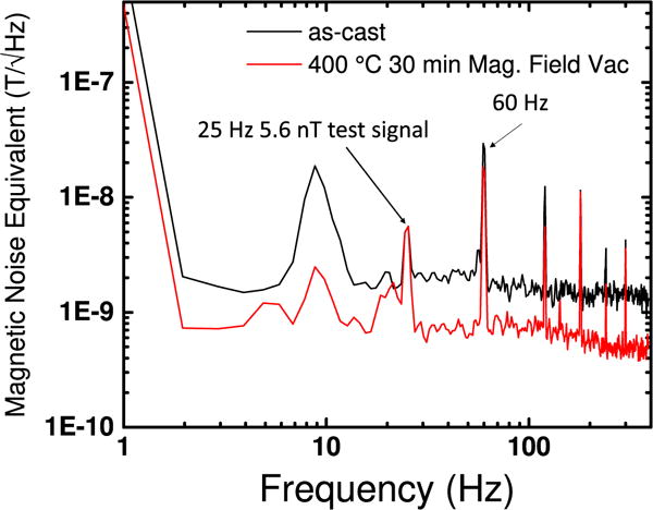
Low frequency noise characteristics of the 6.1 ± 0.03 MV m⁻¹ T⁻¹ device fabricated from Metglas ribbons annealed for 30 min at 400 °C in an applied magnetic field in vacuum and the as-cast sample. A 25 Hz, 5.6 nT sine signal is applied and measured. The 30 min 400 °C with an applied magnetic field in vacuum sample showed a noise floor of approximately 600 pT Hz^−1/2 at 100 Hz, compared to approximately 1.6 nT Hz^−1/2 at 100 Hz for the as-cast sample.

Table 3 shows a comparison of a select set of work showing a range of magnetoelectric magnetometers. The magnetoelectric coefficient and ultimately the limit of detection are determined by a wide range of factors such as the magnetostriction coefficient, piezoelectric coefficient, sensing mode, volume ratios of the layers (for optimal deflection), the coupling coefficient of the epoxy, and noise suppression methods. In this work we choose PZT-5A in the d₃₁ sensing mode as a test vehicle to demonstrate the benefits of optimizing the magnetostrictive material properties because of the simpler fabrication process compared to d₃₃ devices and low cost and availability of PZT-5A compared to PMNPT. The optimized magnetoelectric coefficient is comparable to other d₃₁ sensing devices with PZT (table 3 no. 4–5). The d₃₃ devices that show the highest magnetoelectric coefficient also have high magnetoelectric coefficients with the lowest limit of detection table 3 no. 1–3). The device from table 3 no. 2 shows a very low limit of detection of 2.8 pT Hz^−1/2 but only has a magnetostriction coefficient of 22 μm m⁻¹ mT⁻¹, about 1/3 of the 79.3 μm m⁻¹ mT⁻¹ achieved in this work. This implies that a direct substitution of the optimized Metglas presented in this paper can be used to demonstrate the first sub 1 pT Hz^−1/2 at 1 Hz magnetoelectric magnetometer.

Table 3.

Brief summary of some magnetoelectric magnetometers showing a range of materials and performance metrics. The ME devices fabricated with the optimized ribbons is comparable to other d₃₁ ME devices in terms of α_me and the limit of detection.

No.	Material	Sensing mode	αme MV m−1 T−1	Limit of detection	$\left(\frac{\partial \lambda }{\partial B}\right)$ (μm m−1 mT−1)
1[31]	Terfenol-D/PMNPT	d33	2.5 @ 1 kHz	10 pT @ 1 Hz	12
2[15]	Metglas/PMNPT	d33	52 @ 1Hz	2.8 pT Hz−1/2	22
3[40]	Metglas FeBSiC/PZT-5A	d33	22 @ 1 Hz	N/A	40
4[6]	Terfenol-D/PZT-4	d31	4.68 @ 1 kHz	N/A	N/A
5[8]	Terfenol-D/PZT	d31	0.6 @ 0.5Hz	1.0 nT Hz−1/2 @ 1 Hz	N/A
6(this work)	Metglas 2605SA1/PZT-5A	d31	6.1 @ 20 Hz	0.6 nT Hz−1/2 @ 100 Hz	79

5. Conclusion

We show that easy axis alignment and stress relief in Metglas 2605SA1 ribbons produced by annealing at 400 °C in an applied magnetic field of 160 mT, in a vacuum or N₂ environment improves the magnetoelectric performance by more than a factor of 3 relative to untreated ribbons resulting in a magnetoelectric coefficient measured was 6.1 MV m⁻¹ T⁻¹. An optimal magnetostriction of 50.6 μm m⁻¹ and magnetoelectric coefficient of 79.3 μm m⁻¹ mT⁻¹ were measured. We find that the presence of oxygen degrades samples annealed in air, so an inert or vacuum annealing environment is necessary for achieving the optimal magnetoelectric performance in Metglas 2605SA1 based magnetoelectric sensors. Using a laser vibrometer this paper reports direct measurement of magnetostriction in Metglas films treated under various anneals and in various environments. We also report on SEMPA imaging of domain alignments under various anneals and in various environments.

Table 2.

Oxide thickness profile derived from XPS data. The oxide thickness has an uncertainty of 1 nm due to the finite step size of the Ar etching.

Anneal time (min)	Environment	Oxide thickness (nm)
0 (as-cast)	N/A	3.9
30	Atm.	6.7
60	Atm.	7.6
30	Vac.	4.6
60	Vac.	5.5
60	N2	3.3

References

- 1.Astrov DN. Sov Phys-JETP. 11(1960):708. [Google Scholar]
- 2.Rado GT, Folen VJ. Phys Rev Lett. 1961;7:310–1. [Google Scholar]
- 3.Boomgaard JVD, Van Run AMJG, Van Suchtelen J. Ferroelectrics. 1976;10:295–8. [Google Scholar]
- 4.Van Den Boomgaard J, Terrell DR, Born RAJ, Giller HFJI. J Mater Sci. 1974;9:1705–9. [Google Scholar]
- 5.Van Run AMJG, Terrell DR, Scholing JH. J Mater Sci. 1974;9:1710–4. [Google Scholar]
- 6.Ryu J, Carazo AV, Uchino K, Kim HE. Japan J Appl Phys. 2001;40:4948. [Google Scholar]
- 7.Ryu J, Priya S, Uchino K, Kim HE. J Electroceram. 2002;8:107–19. [Google Scholar]
- 8.Xi H, Qian X, Lu MC, Mei L, Rupprecht S, Yang QX, Zhang QM. Sci Rep. 2016;6:29740. doi: 10.1038/srep29740. [DOI] [PMC free article] [PubMed] [Google Scholar]
- 9.Holmes HR, DeRouin A, Wright S, Riedemann TM, Lograsso TA, Rajachar RM, Ghee Ong K. Smart Mater Struct. 2014;23:095036. [Google Scholar]
- 10.Tan EL, Pereles BD, Horton B, Shao R, Zourob M, Ong KG. Sensors. 2008;8:6396–406. doi: 10.3390/s8106396. [DOI] [PMC free article] [PubMed] [Google Scholar]
- 11.Wang L, Yuan FG. Smart Mater Struct. 2008;17:045009. [Google Scholar]
- 12.Reis S, Silva MP, Castro N, Correia V, Rocha JG, Martins P, Lasheras A, Gutierrez J, Lanceros-Mendez S. Smart Mater Struct. 2016;25:085028. [Google Scholar]
- 13.Gibbs MRJ, Squire PT, Brugel D, Hardy SC, Willson J. J Appl Phys. 1987;61:3784. [Google Scholar]
- 14.Wang Y, Gray D, Berry D, Gao J, Li M, Li J, Viehland D. Adv Mater. 2011;23:4111–4. doi: 10.1002/adma.201100773. [DOI] [PubMed] [Google Scholar]
- 15.Li M, Gao J, Wang Y, Gray D, Li J, Viehland D. J Appl Phys. 2012;111:10–3. [Google Scholar]
- 16.Wun-Fogle M, Savage HT, Spano ML. J Mater Eng. 1989;11:103–7. [Google Scholar]
- 17.Kobelev NP, Soifer YM, Shteinberg VG, Levin YB. Phys Status Solidi a. 1987;102:773–80. [Google Scholar]
- 18.Brouha M, van der Borst J. J Appl Phys. 1979;50:7594. [Google Scholar]
- 19.Berry BS, Pritchet WC. Phys Rev Lett. 1975;34:1022–5. [Google Scholar]
- 20.Meeks SW, Hill JC. J Appl Phys. 1983;54:6584–93. [Google Scholar]
- 21.Livingston JD. Phys Status Solidi A. 1982;70:591–6. [Google Scholar]
- 22.Bucholtz F, Koo K, Dandridge A, Sigel G. J Magn Magn Mater. 1986;54–57:1607–8. [Google Scholar]
- 23.Cadogan JM, Campbell SJ, Jing J, Foley CP, Kater P, Mai YW. Hyperfine Interact. 2014;226:7–14. [Google Scholar]
- 24.Yang Y, Gao J, Wang Z, Li M, Li JF, Das J, Viehland D. Mater Res Bull. 2011;46:266–70. [Google Scholar]
- 25.Metglas. Magnetic alloy 2705m Tech Rep. Metglas, Inc; Conway, South Carolina: 2003. [Google Scholar]
- 26.Datta A, Nathasingh D, Martis RJ, Flanders PJ, Graham CD. J Appl Phys. 1984;55:1784–6. [Google Scholar]
- 27.Metglas. Tech Rep. Metglas, Inc.; Conway, South Carolina: 2011. Amorphous alloys for transformer cores. [Google Scholar]
- 28.Clark A, Crowder D. IEEE Trans Magn. 1985;21:1945–7. [Google Scholar]
- 29.Kellogg RA. PhD Thesis. Iowa State University; 2003. Development and modeling of iron–gallium alloys. [Google Scholar]
- 30.Hatipoglu G, Tadigadapa S. J Appl Phys. 2015;118:034508. [Google Scholar]
- 31.Dong S, Zhai J, Bai F, Li JF, Viehland D. Appl Phys Lett. 2005;87:062502. [Google Scholar]
- 32.Scheinfein MR, Unguris J, Kelley MH, Pierce DT, Celotta RJ. Rev Sci Instrum. 1990;61:2501. [Google Scholar]
- 33.Zhu Y, editor. Modern Techniques for Characterizing Magnetic Materials. New York: Springer; 2005. [Google Scholar]
- 34.Freeman E, Harper J, Goel N, Schiff SJ, Tadigadapa S. Optimization of Metglas 2605SA1 and PZT-5A magnetoelectric laminates for magnetic sensing applications. 2016 IEEE SENSORS. 2016:1–3. doi: 10.1109/ICSENS.2016.7808845. [DOI] [PMC free article] [PubMed] [Google Scholar]
- 35.Kronmüller H, Fähnle M, Domann M, Grimm H, Grimm R, Gröger B. J Magn Magn Mater. 1979;13:53–70. [Google Scholar]
- 36.Pankhurst Qa, Jiang JZ, Betteridge S, Gibbs MRJ, Gehring Ga. J Phys: Condens Matter. 1995;7:9571–93. [Google Scholar]
- 37.Xu J, Atzmon M. Appl Phys Lett. 1998;73:1805–7. [Google Scholar]
- 38.Huang B, Perez R, Crawford P, Nutt S, Lavernia E. MRS Proc. 1995;400:227. [Google Scholar]
- 39.Dussault D, Neste AV, Trudeau ML, Schulz R. The influence of oxygen on the crystallization process of amorphous powders by mechanical deformations. In: Capus JM, German RM, editors. Properties of Emerging P/M Materials. Princeton NJ: Metal Powder Industries Federation; 1992. pp. 13–21. [Google Scholar]
- 40.Dong S, Zhai J, Bai F, Li JF, Viehland D. Appl Phys Lett. 2005;87:062502. [Google Scholar]