Discrete modes of social information processing predict individual behavior of fish in a group

Significance

The way that individuals interact and coordinate their motion in a group is fundamental to the nature of individual and group behavior. Here, we inferred interaction rules that govern individual swimming behavior of adult zebrafish in a group. We show that fish alternate between apparent “active” and “passive” behavioral modes, which we describe using mode-dependent spatiotemporal models of social and sensory computation. This modeling framework closely matches the behavior of individual fish in a group, surpassing previously suggested models that use a universal, ongoing computation. We conclude that group behavior depends on both the computation used by the fish and their current behavioral mode and that the way that fish alternate between modes can shape collective behavior of the group.

Abstract

Individual computations and social interactions underlying collective behavior in groups of animals are of great ethological, behavioral, and theoretical interest. While complex individual behaviors have successfully been parsed into small dictionaries of stereotyped behavioral modes, studies of collective behavior largely ignored these findings; instead, their focus was on inferring single, mode-independent social interaction rules that reproduced macroscopic and often qualitative features of group behavior. Here, we bring these two approaches together to predict individual swimming patterns of adult zebrafish in a group. We show that fish alternate between an “active” mode, in which they are sensitive to the swimming patterns of conspecifics, and a “passive” mode, where they ignore them. Using a model that accounts for these two modes explicitly, we predict behaviors of individual fish with high accuracy, outperforming previous approaches that assumed a single continuous computation by individuals and simple metric or topological weighing of neighbors’ behavior. At the group level, switching between active and passive modes is uncorrelated among fish, but correlated directional swimming behavior still emerges. Our quantitative approach for studying complex, multimodal individual behavior jointly with emergent group behavior is readily extensible to additional behavioral modes and their neural correlates as well as to other species.

Group behavior has been studied in a wide range of species—bacteria (1), insects (2–4), fish (5–11), birds (12–15), and mammals (16–19)—seeking the design principles of collective information processing, decision making, and movement. Theoretical models have suggested possible classes of computations and interaction rules that generate complex collective behavior, qualitatively replicating macroscopic features of behavior observed in real animal groups (20–26), and also have algorithmic, behavioral, and economic implications (27, 28). The ability to record the movement patterns of animals in a group with high temporal and spatial precision for long periods (9, 12, 14, 16, 29, 30) allows for direct exploration of individual traits and interactions between group members. Such attempts have considered topological vs. metric relations between conspecifics (14), effective social “forces” depending on the distance between individuals (5, 6), inference of functional interactions based on maximum entropy models of observed directional correlations (13), hierarchical spatial ordering (12, 31, 32), and active signaling (33, 34).

Because individual behavior is complex, most studies have focused on modeling various statistics of the group, like polarization or moments of the distribution of interindividual distances (7, 14, 35–37). These approaches, however, do not necessarily give a clear or a unique solution for the underlying interactions between individuals (38). Furthermore, in many cases, the suggested models were nonphysiological in terms of response times or temporal causality; ignored physical constraints, such as momentum and friction; or omitted the role of nonsocial sensory information. Somewhat surprisingly, most models of individual behavior in a group assume that animals continuously update their movement based on the location or velocity of their neighbors (20–24, 37). However, characterization of movement patterns of individual zebrafish larva, Caenorhabditis elegans, and Drosophila, for example, suggests that a relatively small set of distinct stereotyped “modes” underlies complex individual behavior (39–41).

Here, we incorporated the concept of discrete behavioral modes in individual animals into a mathematical framework for animal motion in an interacting group. We studied individual behavior in groups of adult zebrafish in a large arena using high spatiotemporal individual tracking under different behavioral contexts. Adult zebrafish live in nature in groups of 4–20 fish, either in still waters or in running rivers (42), and exhibit social behaviors and shoaling tendencies both in the wild and in the laboratory (8, 42). We analyzed the behavior of individuals in the group and identified distinct behavioral modes, which were used to build a highly accurate mathematical model of swimming behavior of individual fish in a group. The model was based on the sensory and social information that was available to each animal and took into account spatial and temporal biophysical constraints. Importantly, we evaluated the models in terms of their power to predict the trajectories of individual fish rather than statistical averages over the whole group (43, 44) and analyzed how behavioral modes of individuals relate to emergent collective behavior of the group.

Results

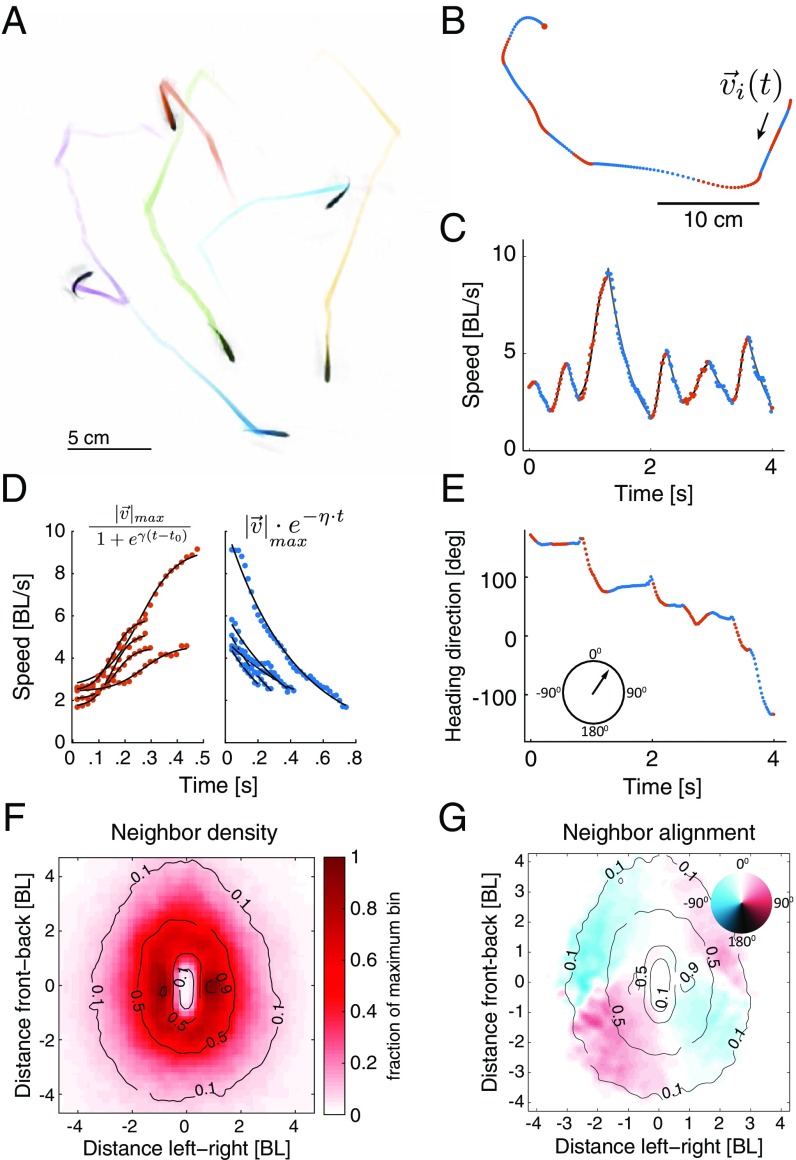
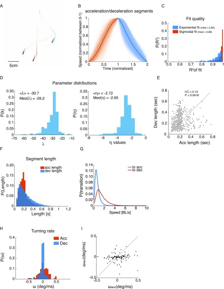
To study individual computations and interactions underlying group behavior in zebrafish, we tracked individuals in groups of 2, 3, 6, and 12 adult fish for up to 1 h at a time in a large circular arena with shallow waters constituting an effective 2D environment (Fig. 1A, SI Materials and Methods, Fig. S1A, and Movie S1). We sampled the trajectory of the center of mass of each fish $i$ in the group, denoted as ${\overrightarrow{x}}_i\left(t\right)$, with high spatial and temporal resolution (SI Materials and Methods) and decomposed the time-dependent velocity of each fish, ${\overrightarrow{v}}_i\left(t\right)$, into instantaneous swimming speed, $s_i\left(t\right)=\left|{\overrightarrow{v}}_i\left(t\right)\right|,$ and instantaneous direction ${\overrightarrow{d}}_i\left(t\right)={\overrightarrow{v}}_i\left(t\right)/\left|{\overrightarrow{v}}_i\left(t\right)\right|$. This revealed a clear segmentation of the trajectories into acceleration and deceleration epochs, which we defined using the maxima and minima points of the speed profile (Fig. 1 B and C, SI Materials and Methods, and Movie S2). Acceleration epochs of the fish were very accurately described by a family of sigmoid functions that differed by their slope and duration (Fig. 1 C and D). Decelerations were very accurately described by a single exponential, corresponding to a simple drag force (Fig. 1 C and D and Fig. S1 B–D). We found that durations of successive epochs of acceleration [$200\pm 104$ ms (mean $\pm$ SD)] and deceleration ($250\pm 160\hspace{0.17em}\text{ms}$) were very weakly correlated, that the rate of switching between them was strongly related to the speed of the fish (Fig. S1 E–G), and that fish made turns mostly during acceleration epochs (Fig. 1E, Fig. S1 H and I, and Movie S2). We note that the continuous motion of the adult fish makes these kinematic states very different from the distinct stop-and-go bouts of zebrafish larvae (45). The segmentation of fish kinematics into clear epochs that have simple functional forms suggests that fish may not be using a universal ongoing computation to determine their behavior at every time instant, as has been suggested previously (7, 23, 24). Furthermore, we find clear anisotropies in group structure, implying that simple distance-based or topology-based models of social interactions, common in the literature, may fall short in explaining individual zebrafish trajectories (14, 21–24): fish prefer to be on the side of other fish within ∼1.5 body lengths (Fig. 1F) and typically showed aligned swimming directions when they are directly in front, behind, or on the side of another fish (Fig. 1G).

Fig. 1.

Kinematic states of individual fish and group structure. (A) Snapshot of the tracks of six freely swimming fish in the arena. (B) A segment of the swimming pattern of a single fish from the group down-sampled for visualization (dots). Dot colors indicate acceleration (red) or deceleration (blue). (C) Speed profile of the trajectory in B. BL, body length. (D) Functional fits to the acceleration and deceleration epochs in C (SI Materials and Methods). (E) Heading direction vs. time for the segment shown in B (Fig. S1H). (F) Density map of neighboring fish relative to a focal fish situated at [0,0] pointing up. (G) Density map of directional alignment of neighboring fish relative to the direction of motion of the focal fish. The color at each point shows the mean alignment value of fish in that bin, with zero representing perfect alignment (SI Materials and Methods).

Fig. S1.

Kinematic states of individual fish in a group. (A) A snapshot of the tracks of three fish. (B) All acceleration and deceleration epochs for a single fish over 5 min of swimming, with time normalized between zero and two (one marks the transition from acceleration to deceleration) and speed normalized between zero and one. Bold lines are the means over all epochs. (C) Distributions of $R^2$ values for all of the segments shown in B, with median values of $0.99$ for accelerations and $0.95$ for decelerations representing high model fit accuracies. (D) Fitted parameters for accelerations (Left) and decelerations (Right). Sigmoid slope $\gamma$ shows that a distribution peaked around $-30\left[1/10\hspace{0.17em}\text{ms}\right]$ and that a friction coefficient peaked around $\eta =-2.7\left[1/10\hspace{0.17em}\text{ms}\right]$. (E) Duration of successive acceleration and deceleration epochs (shown in B) plotted one against the other shows a very weak linear relationship between the two [Pearson’s correlation coefficient (CC) = 0.13, P = 0.0016]. (F) Distributions of acceleration and deceleration durations for all fish in all groups. Acceleration epochs had a mean duration of $\sim 200\pm 104\hspace{0.17em}\text{ms}$ and were generally shorter than decelerations with a mean duration of $\sim 250\pm 160\hspace{0.17em}\text{ms}$. (G) Probability of switching states as a function of swimming speed. As can be expected, the probability of switching from deceleration to acceleration is higher for low-speed values, with a peak at 0.45 body lengths (BLs)/s, a narrow distribution (middle 95% of the distribution between 0.05 and 1.85 BLs/s), while switching back to deceleration is peaked at 1 BLs/s, with a much wider distribution (middle 95% of the distribution between 0.2 and 4.15 BL/s). (H) Distributions of the angular velocity $\omega =d\theta /dt$, with $\theta$ being the heading of the fish, for the acceleration and deceleration epochs shown in B. Note the narrow distribution centered around zero for decelerations. (I) Angular velocity $\omega$ of successive acceleration and deceleration epochs. No clear relationship seems to exist between successive epochs.

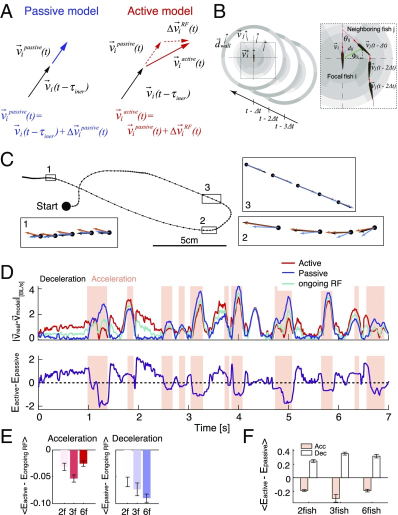
We, therefore, modeled the velocities of individual fish in a group using two behavioral modes: a “passive” mode where inertia and friction control the movement of the fish, with no sensory or social influence, and an “active” mode where an additional sensory term, described by a spatiotemporal receptive field (RF) model of sensory and social processing, contributes to the change in velocity. Discretizing time into $\mathrm{\Delta }t$ bins and denoting the measured instantaneous change in velocity of fish $i$ as $\mathrm{\Delta }{\overrightarrow{v}}_i\left(t\right)$, we modeled the change in velocity in the passive mode as “gliding” where water friction slows down the fish (Fig. 2A):

$$\mathrm{\Delta }{\overrightarrow{v}}_i^{\text{passive}}\left(t\right)=-\eta {\overrightarrow{v}}_i\left(t-{\tau }_{iner}\right),$$ [1]

where $\eta$ is the friction coefficient, estimated from fitting deceleration epochs (Fig. 1D and SI Materials and Methods), and ${\tau }_{iner}$ is a short time constant (chosen here to be 50 ms). In the active mode, we assumed that sensory information and social interactions are taken into account by the fish, and the change in velocity of fish $i$ at time $t$ is given by

$$\mathrm{\Delta }{\overrightarrow{v}}_i^{\text{active}}\left(t\right)=\mathrm{\Delta }{\overrightarrow{v}}_i^{\text{passive}}\left(t\right)+\mathrm{\Delta }{\overrightarrow{v}}_i^{RF}\left(t\right),$$ [2]

where the interaction term $\mathrm{\Delta }{\overrightarrow{v}}_i^{RF}\left(t\right)$ is given by a spatiotemporal RF model (Fig. 2B):

$$\mathrm{\Delta }{\overrightarrow{v}}_i^{RF}\left(t\right)={\displaystyle \sum _{j,k}}{\beta }_j\left(k\right)\cdot {\overrightarrow{v}}_j\left(t-k\mathrm{\Delta }t\right)+{\displaystyle \sum _{l,k}}{\beta }_l\left(k\right)\cdot {\overrightarrow{d}}_l\left(t-k\mathrm{\Delta }t\right).$$ [3]

The first term is a social interaction term summing over the past swimming velocities of neighboring fish, where the weights of spatial bin $j$ at time $t-k\mathrm{\Delta }t$ are given by ${\beta }_j\left(k\right)$, and ${\overrightarrow{v}}_j\left(t-k\mathrm{\Delta }t\right)$ is the velocity of the fish in that bin. The second term is the contribution of nonsocial sensory information, where ${\overrightarrow{d}}_l\left(t-k\mathrm{\Delta }t\right)$ is a vector tangent to the wall closest to the fish, and ${\beta }_l\left(k\right)$ are the weights associated with that bin. Models were fit on labeled training data from acceleration epochs; the number of spatial bins and the extent of the temporal history, which determine the number of parameters, were chosen to maximize model performance on held out test data using penalized regularization (SI Materials and Methods).

Fig. 2.

Modeling fish behavior using active and passive models of social information processing. (A) In the passive model, the change in velocity, Δv_i(t), is given by inertia and friction. In the active model, Δv_i(t) is the sum of the passive component and the contribution of the sensory and social components. (B) The sensory and social components of the active model are described by a spatiotemporal RF, where the behavior of conspecifics in spatial “bins” is weighed with time-dependent parameters (B, Inset and in the text). (C) Example of a trajectory of one fish in a group of three, with a comparison of model predictions (passive model in blue and active model in red) and the measured velocity (black). Insets zoom in on representative segments of the trajectory. (D, Upper) Prediction errors, E_model = |v_real − v_model|, as a function of time for one fish in a group of three using the active model (red), the passive model (blue), and a single RF model trained on data from both states (cyan). Background color designates whether the fish was accelerating (pink) or decelerating (white). BL, body length. (D, Lower) The difference between the errors of the active (red) and passive (blue) models, showing that each of the two models is much more accurate in one of the kinematic states. (E) Average values of difference between errors of the ongoing RF model trained on both states and the active model during acceleration epochs (Left) or the passive model during deceleration epochs (Right) for groups of two, three, and six fish (n = 6, 7, and 7, respectively); error bars represent SEM. (F) Average values of the difference between errors of the active and passive models shown in C (same group sizes as in E).

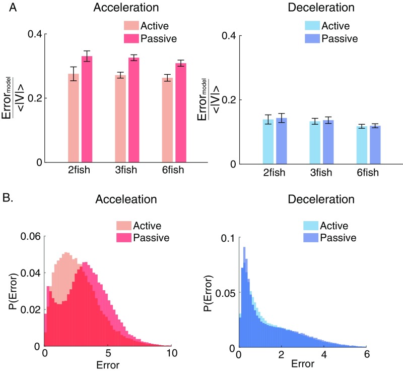
The passive and active models give very different predictions for ${\overrightarrow{v}}_i\left(t\right)$ at different times along the trajectory of a fish swimming in a group. Fig. 2C shows examples of the different predictions of the two models on top of a segment of the swimming trajectory of one fish in a group of three. Fig. 2D shows the models’ prediction errors as a function of time on a short segment of held-out test data, reflecting that the passive model makes smaller errors mostly during decelerations, whereas the active model makes smaller errors mostly during accelerations. This observation was further supported by analyzing complete fish trajectories and multiple groups of the same size recorded independently (n = 6–7 for the different sizes): the active model significantly outperformed the passive model in acceleration epochs, while the passive model outperformed the active model in deceleration epochs (Fig. 2F) (P < 0.0005 for all group sizes, t test for matched samples). Learning a separate RF model for the deceleration epochs did not result in a significant improvement over the passive model (Fig. S2), reasserting that fish show very weak social responses during decelerations. To compare our results with the common notion of a single ongoing computation by individuals in a group, we also fitted a single spatiotemporal receptive field model that was trained on data from both epochs. This “ongoing RF” model was significantly worse than the active model for the acceleration epochs and the passive model in deceleration ones (Fig. 2 D and E) (P < 0.005 for all group sizes in both kinematic states, t test for matched samples). These results indicate that individual fish alternate between two distinct modes of social information processing, which roughly correspond to the kinematic state of the fish. (While it seems that, in the passive state, the fish ignore their neighbors, the fish probably still collect social and sensory information during these epochs, and therefore, we refer to both the active and passive modes as “information processing states.”)

Fig. S2.

Error analysis confirms that fish show little social response during decelerations. (A) Comparison of the normalized error in prediction $\left|{\overrightarrow{v}}_{\text{model}}-{\overrightarrow{v}}_{\text{real}}\right|/\langle \left|{\overrightarrow{v}}_{\text{real}}\right|\rangle$ during acceleration epochs (Left) and deceleration epochs (Right) using an active model—an RF model learned separately on each kinematic state (Eq. 3) and a passive model (Eq. 1). There is no advantage in learning a separate RF model to predict active movements in the deceleration epochs. (B) Example distributions of the errors $\left|{\overrightarrow{v}}_{\text{model}}-{\overrightarrow{v}}_{\text{real}}\right|$ in prediction during acceleration epochs (Left) and deceleration epochs (Right) for the two models as in A; again, error distributions in the deceleration epochs are similar for active and passive computation in these parts.

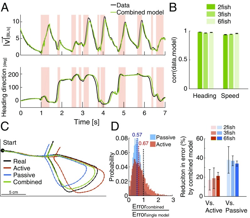
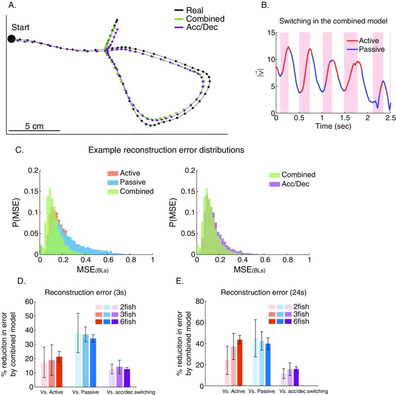
Since we do not have access to the internal state of information processing of the fish, we asked how well we could explain fish behavior if we were to pick the best model for each time point (the one that gives the lowest error compared with the real velocity). This combined model (Movie S3) gives an excellent fit to the data both in terms of the speed (Fig. 3A, Upper) and the heading direction of swimming (Fig. 3A, Lower). Over all groups, the correlations between the real and the estimated velocity of the fish were ∼0.97 for direction and ∼0.94 for speed on test data (Fig. 3B). To further illustrate the importance of the two interleaved modes for describing individual behavior, we compared the accumulated effect of the errors in predicting the instantaneous velocity vectors that each of the models makes. Fig. 3C shows the “reconstructed” swimming trajectory of a fish in a group that would result from summing over the instantaneous velocity predictions of each model to obtain a complete trajectory segment (SI Materials and Methods). Repeating this analysis for 5,000 3-s-long segments of a group of three fish, we found that combining the active and passive models gave much more accurate reconstructions than either model alone (Fig. 3D, Left and Fig. S3C). The reconstruction errors over trajectory segments for all groups of three fish were lower by $37\pm 5\%$ compared with the passive model alone and $19\pm 11\%$ compared with the active model alone, with similar results for groups of two and six fish (Fig. 3D, Right) (P < 0.005 for all group sizes and for both comparisons, t test for matched samples). While this combined model is an upper bound on the performance of any mix of the active and passive models, similar performance gains are retained in a model where the active and passive models are chosen according to the kinematic state of the fish (Fig. S3).

Fig. 3.

Accurate prediction of velocity and fish trajectory reconstruction. (A) Examples of the measured speed (Upper) and heading direction (Lower) of a single fish in a group of three (black) and the prediction of the combination of the active and passive models, picking the better model at each time point (green). BL, body length. (B) Average correlation between measured speed and heading direction and model predictions for all fish in groups of the same size (error bars = SEM; n = 6, 7, and 7 groups). (C) A short segment (3 s) of the trajectory of a fish in a group of three (black) and the reconstructed trajectory obtained by accumulating the velocity predictions of the active model (red), the passive model (blue), and the optimal combination of the two (green) (SI Materials and Methods). (D, Left) Distribution of the ratio between the reconstruction errors of the combined model and those of the active model or the passive one alone for 5,000 segments similar to the one shown in C. Values below one (black dashed line) represent advantage to the combined model. Colored dashed lines mark the corresponding distribution medians. (D, Right) Average reduction in prediction error of the combined model vs. the active model or the passive model alone for groups of different sizes; error bars represent SD.

Fig. S3.

Switching in the combined model is comparable with the kinematic state of the fish. (A) The trajectory segment from Fig. 3C (black) and the predicted trajectory using the optimal combination of the two models (green) overlaid with the predicted trajectory based on switching between models that is done according to the acceleration or deceleration state of the fish (purple). (B) An example of the optimal switching between models in the reconstruction shown in Fig. 3C and A (green line) and their high correspondence to the acceleration/deceleration state of the fish (pink background represents accelerations). (C, Left) Example distributions of the reconstruction error $\text{MSE}={\displaystyle \sum \left|{\overrightarrow{c}}_{\text{model}}-{\overrightarrow{c}}_{\text{real}}\right|/N}$ using the combined model (green) compared with the active (red) and passive (blue) models. BLs, body lengths. (C, Right) Comparison of the combined model (green) with switching according to the acceleration/deceleration state of the fish (purple). (D) Average reduction in the reconstruction error of the combined model compared with the active model alone (red), the passive model alone (blue), and the prediction obtained by switching according to the acceleration/deceleration state of the fish (purple). Error bars represent SD. (E) Similar to D only for reconstruction of longer trajectory segments (24 s), giving highly similar results.

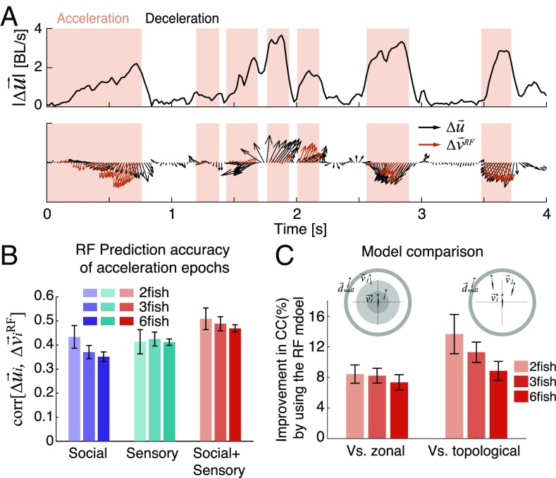
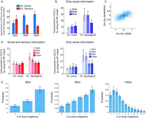
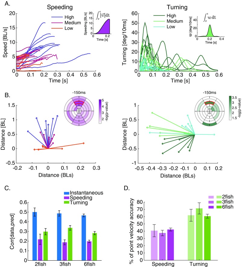
A significant part of the high correlation between model predictions and the data originates from the autocorrelation of individual swimming behavior. This is especially true in deceleration epochs, where the correlation between the measured ${\overrightarrow{v}}_i\left(t\right)$ and prediction based on $\mathrm{\Delta }{\overrightarrow{v}}_i^{\text{passive}}\left(t\right)$ was $0.986\pm 0.002$ (low prediction error values in Fig. S2A). We, therefore, focused on the change in velocity that is not explained by autocorrelation and friction: Fig. 4A shows the change in velocity that is not explained by the passive component, which we denote as $\mathrm{\Delta }{\overrightarrow{u}}_i\left(t\right)=\mathrm{\Delta }{\overrightarrow{v}}_i\left(t\right)-\mathrm{\Delta }{\overrightarrow{v}}_i^{\text{passive}}\left(t\right)$. Clearly, in the deceleration epochs, removing the passive component leaves very little change to explain. In the acceleration epochs, the correlation between $\mathrm{\Delta }{\overrightarrow{u}}_i\left(t\right)$ and the prediction of $\mathrm{\Delta }{\overrightarrow{v}}_i^{RF}\left(t\right)$ was ∼0.5. When we examined the social or sensory contributions to the RF model in isolation, the prediction performance was significantly lower than when both were included (Fig. 4B) (P < 0.0005 for all group sizes, t test for matched samples), with small differences between group sizes (Fig. S4A). The nonadditivity of social information and nonsocial sensory information reflects the redundancy between them. In this setup, it is impossible to discern whether fish “read” sensory information about the environment from their own senses or from the behavior of other fish. We note that the relation between $\mathrm{\Delta }{\overrightarrow{v}}_i$ and the predictions of the models did not indicate a need for a nonlinear extension of the RF model (Fig. S4C) [compare with linear–nonlinear models in neuroscience (46)]. Predicting the entire acceleration epoch using a similar RF model from the sensory and social information at the beginning of the epoch performed significantly worse (SI Materials and Methods and Fig. S5).

Fig. 4.

Active movement changes are accurately predicted by the RF model using both social and sensory information. (A, Upper) An example of |Δu_i(t)|, the magnitude of the measured change in velocity after subtracting the passive component (in the text) of a single fish in a group of three over 4 s; background colors mark acceleration epochs (pink) and deceleration epochs (white). BL, body length. (A, Lower) Comparison of the measured Δu_i(t) and the prediction obtained using the RF model (red arrows) in the acceleration epochs. (B) Prediction accuracy of Δu_i(t) by RF models that use only the social information component, only the sensory information component, or both components of Eq. 3 for different group sizes (error bars represent SEM; n = 6, 7, and 7 groups). (C) Improvement in predicting Δu_i(t) in acceleration epochs by the RF model relative to the corresponding zonal or topological versions (SI Materials and Methods has details); values are averaged over all groups of different sizes. CC, correlation coefficient; error bars represent SEM.

Fig. S4.

Active movement changes are accurately predicted by the RF model using both social and sensory information. (A) Improvement in prediction accuracy (CC, correlation between data and model) of the RF model using both social and sensory information compared with the social information alone (blue) and sensory information alone (red) for all group sizes (n = 6, 7, and 7; error bars represent SEM). (B) Improvement in prediction accuracy by using the RF model compared with the zonal and topological models when using only sensory information for prediction for all group sizes (n = 6, 7, and 7; error bars represent SEM). (C) Predicted velocity components $\mathrm{\Delta }{v}_x,\mathrm{\Delta }{v}_y$ of $\mathrm{\Delta }\overrightarrow{v}$ plotted against their measured values. The linearity and homogeneity of variance across predicted values suggest that we should expect a limited benefit from adding static nonlinearities to our model. (D) Improvement in prediction accuracy by using the RF model compared with the zonal and topological models. Similar to Fig. 4C and B but also including results of 12 fish groups. (E) Averages (and SEM) of the probability to observe 0 to n − 1 neighbors within a distance of six body lengths from a focal individual for groups of 3, 6, and 12 fish (n = 7, 7, and 6, respectively). This distance was used as the upper limit of neighbor interactions in the RF and zonal models. Note the clear difference in the distributions of close neighbors between groups of 12 fish and groups of 3 and 6 fish. It is rare to find zebrafish in cohesive 12 fish groups.

Fig. S5.

Prediction of complete speeding and turning profiles using RF models. (A) Examples of speeding (Left) and turning (Right) profiles (angular velocity) colored by the strength of the response (“low,” “medium,” and “high”), which was determined by discretizing the integrals of responses (Insets) into evenly sized bins. BL, body length. (B, Insets) RF maps showing bins with significantly different neighboring fish behavior before each of the binned responses depicted in A (SI Materials and Methods). (B) Average velocity vectors of the fish in the bin marked in red in B, Insets for different speeding strengths (B, Left) and turning strengths (B, Right); strength is denoted by color as in A. (C) Comparison of the accuracy of prediction for the instantaneous model when predicting $\mathrm{\Delta }{\overrightarrow{v}}_i\left(t\right)$ (blue) and the accuracy of predicting the complete turning ${\displaystyle {\int }_0^t\omega dt}$ and speeding ${\displaystyle {\int }_0^t\left|\overrightarrow{v}\right|dt}$ profiles (purple and green, respectively). Values are average correlation coefficients (n = 6, 7, and 7), and error bars represent SEM. (D) Prediction accuracy of complete turning and complete speeding responses using social and sensory information preceding these events, represented as percentage of the accuracy of predicting point accelerations [$\mathrm{\Delta }{\overrightarrow{v}}_i\left(t\right)$] using similar data. Indeed, the ability to predict properties of entire acceleration epoch is significantly lower.

Our RF model outperformed common models of collective movement in predicting $\mathrm{\Delta }{\overrightarrow{u}}_i$, even when the parameters of these competing models were optimized for our data (SI Materials and Methods): we predicted $\mathrm{\Delta }{\overrightarrow{u}}_i\left(t\right)$ $\sim 8\pm 2.5\%$ better on average than a “zonal model” (23) and $\sim 11.3\pm 4\%$ better than a “topological model” (14) (Fig. 4C) (P < 0.05 for all group sizes and both model comparisons, t test for matched samples). The advantage of the RF model was even more pronounced when prediction was based only on social information (Fig. S4B). We found similar advantages of the RF model over the zonal and topological models when studying groups of 12 fish (Fig. S4D), but these larger groups do not stay in a cohesive structure for long periods of time (Fig. S4E), effectively breaking up into smaller subgroups.

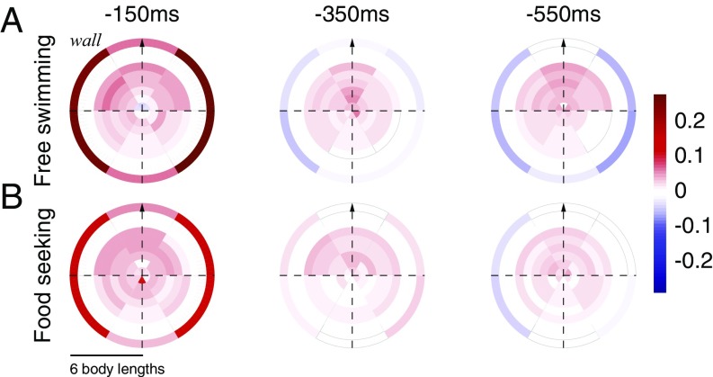
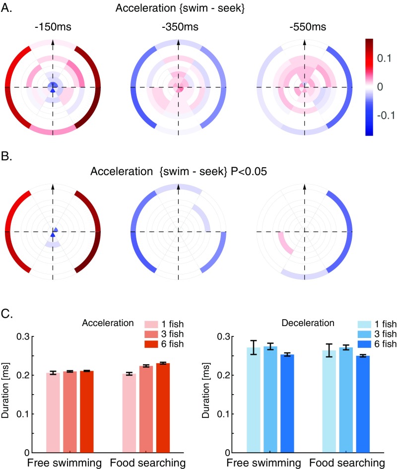
To characterize the spatiotemporal effects of social and sensory information on the movement decisions of a focal fish, we compared the weight maps of the RF models under two different behavioral contexts—fish swimming freely in the arena as described above and fish who were trained to seek food that is randomly scattered in the arena (SI Materials and Methods). Inhomogeneity in the RF map reflects the effects of the relative distance and relative angle of neighbors on the focal fish (Fig. 5A): social effects are strongest in front of the fish and weaker behind it. The weights of the nonsocial information show the opposite structure, with walls directly to the side of the fish having the strongest effect on its behavior. Overall, the effects of neighbors are weaker for longer temporal delays but retain their positive sign, whereas the effect of the wall decreases faster with time (Fig. 5A, Center) and then switches sign. Interestingly, the way that fish integrate information from their surroundings changes with the behavioral context (Fig. 5B): the effects of arena walls are weaker in food-searching fish, and the effects of fish positioned directly behind the focal fish are positive and stronger (Fig. S6 A and B shows statistically significant differences between weight maps). In addition, during food searching, fish in groups (unlike solitary fish) show longer acceleration epochs compared with freely swimming ones (Fig. S6C).

Fig. 5.

RF maps show distinct spatial, temporal, and behavioral state dependencies. (A) RFs for a fish in a group of three fish (n = 7), freely swimming in the arena, for the model illustrated in Fig. 2B (shown are average β values from Eq. 3). Outer circles represent weights associated with the walls of the arena. (B) RFs obtained for a fish in a group of three fish (n = 7) trained to seek food in the arena (no food is present during the analyzed session).

Fig. S6.

RF maps show distinct behavioral state dependencies. (A) Average difference maps of the RF for groups of three fish during acceleration when performing free swimming and food seeking (see above). Bins with weights that were larger in the free swimming state are colored red, and opposite bins are in blue. (B) Same as A but showing only bins with differences that pass a significance test (t test for matched samples, P < 0.05). (C) Average duration of acceleration epochs (Left) and deceleration epochs (Right) in a food-searching task and a free swimming context. Groups of three and six fish show significantly longer accelerations when searching for food, while solitary fish do not exhibit this increase in duration (two-way ANOVA shows significant interaction of size and searching condition comparing groups of either three or six fish with solitary fish, P < 0.02 for both tests). Deceleration epochs show similar durations comparing food-searching and free swimming conditions, although a larger (but consistent) variability exists between the different group sizes (no significant interactions of size and searching condition for groups of either three or six fish compared with solitary fish, P > 0.77 for both). We analyzed the kinematic states of individuals in groups of fish and of solitary fish (from the same batch of experiments) using 16 solitary fish, 10 groups of three fish, and 10 groups of six fish. Food-searching training protocol was the same as the one described in SI Materials and Methods.

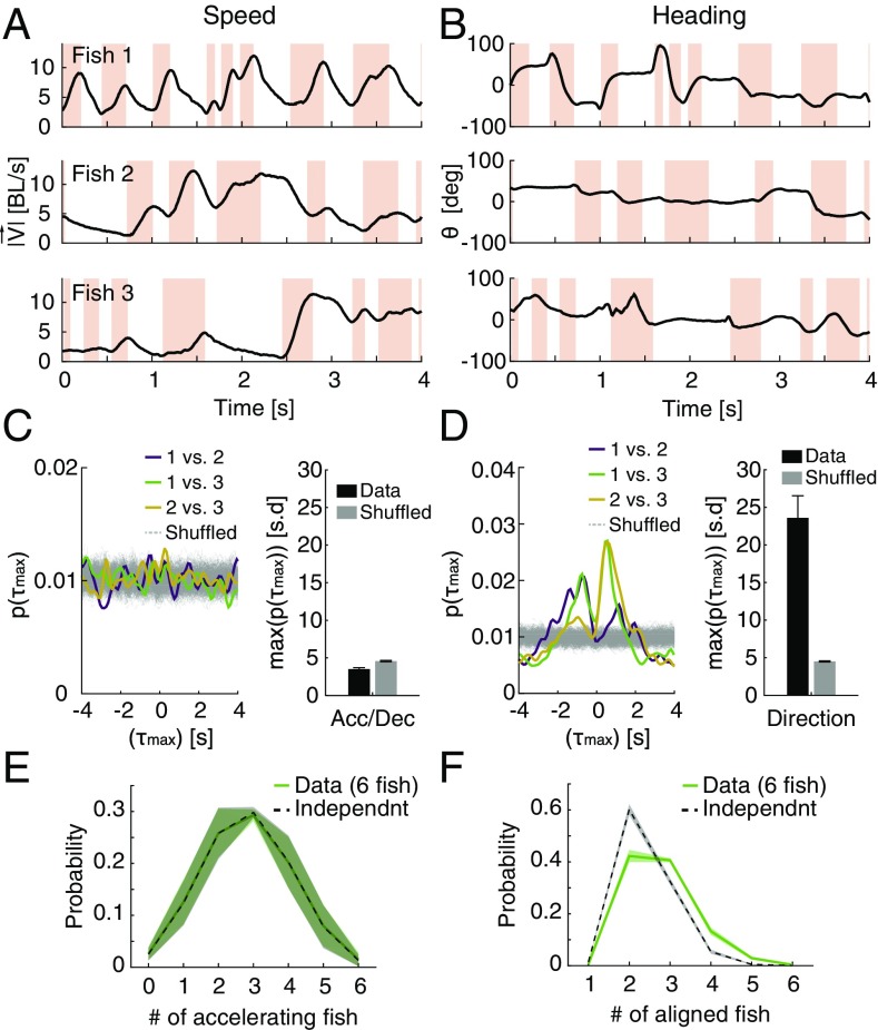
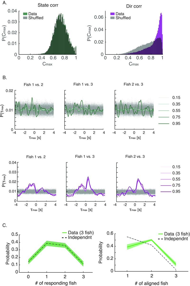
What does switching between the two modes of information processing at the individual level imply for the behavior of the group? Fig. 6 A and B shows an example of the swimming velocities of three fish decomposed into the speed $s_i\left(t\right)$ (Fig. 6A) and the direction of swimming $\theta \left({\overrightarrow{d}}_i\right)$ (Fig. 6B). We asked what the temporal relations were between kinematic states in pairs of fish in the group by seeking the time lag that would maximize the correlation for short movement segments (1-s long) for each fish pair (using ref. 47 to verify the identity of tracked individuals) (SI Materials and Methods). The distribution of the time of maximal correlation $\left({\tau }_{\max }\right)$ was indistinguishable from the expectation of fish changing states independently (Fig. 6C), and correlation values also did not differ from what was expected by chance (Fig. S7A). Such independent transitions between behavioral modes of individual fish could give the group a way to sample the sensory space in a distributed and interleaved manner, with no temporal processing gaps, without the need for scheduling. In contrast, similar analyses identified significant correlations between swimming directions in pairs of fish (Fig. S7A) and a corresponding significant peak in the distribution of temporal lags, suggesting causal relationships (Fig. 6D). The independence of kinematic states among fish with correlated swimming direction was apparent also at the level of the group from the distribution of synchronized states among the fish: namely, the probability to find $k$ of the $N$ fish in the group to be accelerating synchronously (Fig. 6E) and the probability of $k$ fish swimming in a similar direction (Fig. 6F). For synchronous accelerations, the probability distribution was symmetric and matched closely the expected distribution if fish were switching states independently of one another (Fig. 6E). The distribution of number of fish swimming synchronously in the same direction had a clear structure and was very different from the expectation for independent fish (Fig. 6F). Thus, independent switching between modes of information processing in individual fish on a timescale of several seconds is consistent with the emergence of correlated directional behavior with clear temporal ordering at the group level.

Fig. 6.

Asynchronous switching between information processing modes among individual fish in a group and synchronous heading directions of group members. (A) Example of the simultaneous acceleration (pink)/deceleration (white) profiles of three fish in a group. BL, body length. (B) Same as in A but for the heading direction of the fish. (C, Left) Distributions of time difference (τ_max) that gave the maximum correlations between the kinematic states of pairs of fish for 1-s-long windows in a group of three (colored lines) and shuffled controls (light gray) (SI Materials and Methods). (C, Right) Peak values of the distribution of time difference (τ_max) shown in C, Left in units of SDs for pairs of fish and for shuffled data averaged over all pairs of fish within all groups of three fish (n = 6, P = 0.99, t test for matched samples). (D) Same as in C but for the distribution of time difference (τ_max) of the cross-correlation of direction of motion of pairs of fish. Here, directional correlation shows clear structure and peak times (n = 6, P < 0.0005, t test for matched samples). (E) Average empirical probability distribution P(a₁, a₂, …, a_n) of fish kinematic states (acceleration or deceleration), where a_i represents the state of fish i (solid green), and the prediction of a model assuming independence between fish p(a₁)p(a₂) … p(a_n) (dashed line); shadings represent SEM. (F) Similar to E for the distribution of heading direction P(d₁, d₂, …, d_n), where d_i is the direction of fish i discretized into six evenly sized bins (SI Materials and Methods) (solid green), and the distribution obtained under the assumption of independence p(d₁)p(d₂) … p(d_n) (dashed line).

Fig. S7.

Asynchronous switching between information processing modes among individual fish in a group and synchronous heading directions of group members. (A) Distributions of maximal correlation values for a group of three fish (from Fig. 6) for the state correlation analysis (Left) and for the directional correlation analysis (Right) and the correlations obtained using shuffled data in gray (in the text). (B) Distributions of delay time $\left({\tau }_{\max }\right)$ of the maximum correlations between pairs of fish in a group of three (colored lines) and shuffled controls (light gray). Different colors represent different correlation thresholds, where only ${\tau }_{max}$ values corresponding to maximal correlations above these thresholds are used to construct the distributions. For both the state correlation (Upper, green lines) and for directional correlation (Lower, purple lines), using different thresholds does not change the structure of the result presented in Fig. 6. For comparison, shuffled controls are plotted using correlation threshold of 0.95. (C) Group state correlation for groups of three fish, similar to the analysis presented in Fig. 6 E and F for six fish.

SI Materials and Methods

Experimental System.

In total, 147 adult zebrafish (Danio rerio), purchased from Aquazone Israel LTD, with approximately equal male:female ratio were studied (n = 6 groups of 2 fish, n = 7 groups of 3 fish, n = 7 groups of 6 fish, and n = 6 groups of 12 fish). Fish were housed separately in their designated groups for at least 1 mo before experiments. Environmental conditions were constant using a recirculating system and multistage filtration, with water temperature of 27 °C to 28 °C, conductivity of 600–700 $\mu \text{S}$, and pH levels of 7.7–8. Lighting was kept at a 14:10-h light/dark cycle with fluorescent lights. Unless otherwise indicated, fish were fed twice a day a mixture of dry flake food. Experimental arena consisted of a large 1.2- over 1.1-m rectangular aquarium, with circular arenas of different diameters placed in it (Movie S1). Water levels were kept at a depth of about 5 cm to constitute a pseudo-2D environment. Video recording was done using an industrial recording system with a Vieworks VC-2MC-M340 digital camera with an 8-mm lens connected to a Karbon-CL frame grabber. Camera was attached to the ceiling over the test aquarium ≈150 cm above water level to capture the entire arena.

Data Extraction.

Videos were analyzed offline to extract the physical properties of the fish (size, position, orientation). Position data were used to estimate fish trajectories using a designated tracker. All image processing and tracking were done using Matlab with software written in our laboratory. Briefly, fish were first detected as darker blobs over the lighter background, and their physical properties were calculated. Next, the centers of mass of fish were connected frame by frame to give the estimated track of each fish. When several fish were close to one another, an additional step was taken to estimate the most likely number of fish in the large blob and their centers. This tracking method provided accurate detection of fish in >90% of the frames analyzed but did not ensure constant identities of the fish. When needed, fish identities were corrected using the IdTracker software (47). Fish trajectories were smoothed using a Savitzky–Golay filter (56) spanning 33 frames, which constitute ∼1/3 of 1 s. Fish positions were set as the coordinates of the fish center: ${\overrightarrow{c}}_i\left(t\right)=\left[x{\left(t\right)}_i,y{\left(t\right)}_i\right]$, and fish velocity was estimated as the difference between two consecutive points: $\overrightarrow{v}{\left(t\right)}_i=\overrightarrow{c}{\left(t\right)}_i-\overrightarrow{c}{\left(t-1\right)}_i$. Direction of motion of the fish was defined as $\overrightarrow{d}{\left(t\right)}_i=\overrightarrow{v}{\left(t\right)}_i/\left|\overrightarrow{v}{\left(t\right)}_i\right|$ or $\theta {\left(t\right)}_i$ as the angle of $\overrightarrow{d}{\left(t\right)}_i$, and angular velocity was given by $\omega {\left(t\right)}_i=\theta {\left(t\right)}_i-\theta {\left(t-1\right)}_i$. As fish tend to respond strongly to walls of the arena, we did not use data from fish positioned “close” to the boundary—all distances smaller than the median of the wall distance distribution were discarded from further analysis.

Behavioral Experiments.

Free swimming.

Before behavioral experiments, fish were habituated to the circular arena (95-cm diameter) for short sessions of ∼10 min for 2 d. We then filmed their free swimming behavior for 30 or 60 min.

Food seeking.

To train fish to seek for food in the arena, we conducted a 7-d training protocol. On each day, fish were transferred from their home tank to the experimental arena, where a constant number of flakes (∼4 mm in diameter) was scattered randomly on the water surface. Fish were allowed 5 min to consume the flakes, and then, they were netted and returned to their home tanks. To facilitate learning, the effective size of the arena used by the fish was increased over days (from a small box of 25 × 25 cm to circular arenas of diameters of 57, 82, and 95 cm). During training, no other food was given to the fish, and on days 6 and 7, fish were deprived of food. On day 8, fish were transferred again to the test tank, and their behavior was recorded, with no food present.

Kinematic Models of Fish Acceleration and Deceleration Segments.

Segmentation of speed profiles into acceleration and deceleration epochs was done by detecting the minima and maxima of the speed profile using numerical differentiation. To overcome local noise, we constrained two local minima to be separated by at least four frames (or 40 ms), and the single highest extrema between two such minima points was taken as the local maximum point (and end of acceleration). Each segment $j$ of fish $i$ was fitted individually: a single exponential $s_i^{dec\left[j\right]}\left(t\right)=\max \left(s_i^{dec\left[j\right]}\right)\cdot e^{\left(-{\eta }_{ij}\cdot t\right)}$ was used to fit decelerations, and a sigmoid $s_i^{acc\left[j\right]}\left(t\right)=\max \left(s_i^{acc\left[j\right]}\right)/1+e^{{\gamma }_{ij}\left(t-t_0\right)}$ was used for accelerations. Maximum speeds for both models—$\max \left(s_i^{acc\left[j\right]}\right)$ and $\max \left(s_i^{dec\left[j\right]}\right)$—were obtained from the data as was the midpoint of the sigmoidal function $t_0$, leaving the “slope” of both models ${\eta }_{ij}$ and ${\gamma }_{ij}$ as free parameters to be fitted (Fig. S1 B–D). Fitting was done only for segments that were at least 100-ms long (i.e., having at least 10 data points for fitting).

Neighbor Maps.

Neighbor position maps were based on 2D histograms of neighbors’ positions in space relative to a focal fish with orientation that was defined as “North.” Histograms were smoothed using a rotationally symmetric Gaussian low-pass filter [${\sigma }^2=$ 0.13 (body lengths)].

To estimate the neighbor alignment maps, the average direction of motion of fish in each bin was calculated using all instances in which the bin was occupied. The angular deviation of that average vector from the direction of motion of the focal fish was expressed in angles [−180, 180], where positive values represent deviation to the right (“East”) and negative values represent deviation to the left (“West”).

Model Fitting.

RF models were fit using a Lasso least squares regression (57) with cross-validation. Briefly, for a given nonnegative $\lambda$, we calculated

$${\min }_{\overrightarrow{\beta }}\left\{\frac{1}{2N}{\displaystyle \sum _{t=1}^N{\left({\overrightarrow{v}}_t-{\overrightarrow{x}}^T\cdot \overrightarrow{\beta }\right)}^2}+\lambda {\displaystyle \sum _{j=1}^p\left|{\beta }_j\right|}\right\},$$ [S1]

where ${\overrightarrow{v}}_t$ is the empirical velocity of fish in time instance $t$, $\overrightarrow{x}$ is a set of velocities of neighboring fish in the spatiotemporal RF around the fish (Eq. 3), $\overrightarrow{\beta }$ is a vector of model parameters or bin weights (of length p), and N is the total number of observations. Repeating this procedure for different values of $\lambda$, we found the set of parameters $\overrightarrow{\beta }$ that minimized the cross-validation error for held out data. This regularization process usually reduces the effective number of parameters (setting some of the weights to zero), resulting in a sparser model.

Competing Models.

We compared our RF parameterization of space, which depends on both angle and distance of neighbors from the focal fish (Fig. 2B), with two commonly used parameterizations of space: a zonal model (22–24), where only the distance of neighboring fish is taken into account, and a topological model (14), where neighbors are weighed according to their topological order (first neighbor, second neighbor, etc.), ignoring their metric distance (Fig. 4C, Insets shows model sketch). Mathematically, we get a similar expression as in Eq. 3:

$$\mathrm{\Delta }{\overrightarrow{v}}_i^{\text{Model}}\left(t\right)={\displaystyle \sum _{j,k}}{\beta }_j\left(k\right)\cdot {\overrightarrow{v}}_j\left(t-k\mathrm{\Delta }t\right)+{\displaystyle \sum _{l,k}}{\beta }_l\left(k\right)\cdot {\overrightarrow{d}}_l\left(t-k\mathrm{\Delta }t\right),$$ [S2]

where the first term is the social interaction term, but spatial weights are assigned to bins according to their distance from the focal fish (zonal model) or to topological neighbors. Temporal binning was kept similar to that used in the RF model for comparison.

Model Parameters.

Discretization of the RF into spatiotemporal bins and the temporal bins of the topological and zonal models were chosen using a nonexhaustive search of parameter space, whereas zonal model radii were optimized for the cases of either two or three rings. Thus, the RF parameters used here give only a lower bound on the accuracy of this model, since an exhaustive search of the parameter space can optimize the obtained results. All parameters used in the models are listed below.

Parameter name	Meaning	Value used in analysis
For the RF-model
No. of sectors	No. of sectors in the RF	Six sectors
Start angle	The middle point of the first sector with respect to fish motion	0° (North)
No. of rings	No. of rings in the RF	Six rings
Ring size	$R_{i+1}-R_i$, where $R_i$ is the radius of ring i	One body length
For the zonal models
No. of rings	No. of rings in the zonal model	Two rings
Ring size	$R_{i+1}-R_i$, where $R_i$ is the radius of ring i	Three body lengths
Temporal parameters similar for all models
No. of steps back	No. of discrete steps back in time used for prediction	Three steps
$\mathrm{\Delta }{t}_1$, $\mathrm{\Delta }{t}_2$, $\mathrm{\Delta }{t}_3$	Time lag between current focal fish velocity and previous neighbors’ velocities for the three time steps used	150 ms (15 frames), 350 ms (35 frames), 550 ms (55 frames)

Trajectory Reconstruction.

Predicted positions of fish $i$, $C_i\left(t\right)$ over time, were obtained using the instantaneous velocities ${\overrightarrow{v}}_i\left(t\right)$ predicted by the models, where ${\overrightarrow{C}}_i\left(t\right)={\overrightarrow{C}}_i\left(t-1\right)+{\overrightarrow{v}}_i\left(t\right)$; ${\overrightarrow{v}}_i\left(t\right)$ were obtained either by the active model or the passive model (in the text). The “combined model” is where, for each time step t, we use the prediction of the model that gave the lower error $E_{\text{model}}=\left|{\overrightarrow{v}}_{\text{real}}-{\overrightarrow{v}}_{\text{model}}\right|$ between the real and predicted velocities for that time step. We note that this is only a locally “optimal” choice that does not guarantee that the total error between real and predicted trajectories will be minimal.

Directional and Behavioral Cross-Correlation Analysis.

Time-windowed directional cross-correlation (12, 31) was estimated using a short window of the response of fish $i$ ($L=1\hspace{0.17em}\text{s}$) and the responses of fish $j$ over a range $-4\le \tau \le 4$ s (in 10-ms increments):

$$C_{ij}\left(t\right)={\displaystyle \sum _{\tau }}{\overrightarrow{v}}_i\left(t\right){\overrightarrow{v}}_j\left(t-\tau \right),$$

where ${\overrightarrow{v}}_i$ and ${\overrightarrow{v}}_j$ are fish velocities. The time delay $\tau$ that gives the maximal correlation for this segment is then considered to be the temporal relation between animals. We then calculate $C\left(t\right)$ for all time points and for all pairs of fish in a given group and find the maximal correlation for each segment $C_{ij}^{\max }$ (Fig. S7A) and the temporal delay corresponding to this maximal correlation ${\tau }_{\max \left(c\right)}$. Histograms of temporal relations (Fig. 6D and Fig. S7B, Lower) are then constructed using these ${\tau }_{\max \left(c\right)}$ values, keeping only temporal delays of high correlations $C_{ij}^{\max }\ge 0.9$ to focus only on instances where the fish are actually responding to one another but also, to ensure that more that 10% of all correlations are retained both for the actual data and for the shuffled analysis (see below). Importantly, choosing different thresholds for $C_{ij}^{\max }$ did not qualitatively change the results obtained (Fig. S7B, Lower).

Behavioral state correlation was estimated in a similar manner, but in this case, we use $x_i$ and $x_j$, which are binary variables denoting acceleration (one) or decelerations (zero) (Fig. S7A, Left). When constructing the temporal delay distributions (Fig. 6C), we kept ${\tau }_{\max \left(c\right)}$ values corresponding to $C_{ij}^{\max }\ge 0.8$ for the behavioral state correlation as to retain at least 10% of the correlation in the shuffled analysis. Choosing different threshold values for this analysis as well gave similar results (Fig. S7B, Upper).

To obtain a null distribution of expected correlation values, we repeated the same time-windowed cross-correlation analysis as formulated above for both direction and behavioral state but with each fish’s trajectories randomly shifted in time. We repeated this full analysis 1,000 times for each pair of fish (gray lines in Fig. 6 C and D and gray lines in Fig. S7 A and B). To compare the magnitude of the peaks of the time delay distributions $\max \left[P\left({\tau }_{\max }\right)\right]$ found in real pairs and that of the time-shuffled pairs, we normalized the maximal values of $P\left({\tau }_{max}\right)$ using the mean and SD of the maxima found in the repetitions of the shuffled analysis:

$$\text{score}=\frac{\text{peak}-{\mu }_{\text{shuffled}}}{{\sigma }_{\text{shuffled}}},$$

where ${\mu }_{\text{shuffled}}$ and ${\sigma }_{\text{shuffled}}$ are the mean and SD of the peak in the shuffled data. In this way we are effectively conducting a bootstrap analysis comparing the maximal probability in our data with that found in the shuffled analysis (Fig. 6 C, Right and D, Right).

Estimating Empirical Distributions of Collective States.

We evaluated the joint probability distributions of synchronous fish states, $P\left(a_1,a_2,\dots ,a_n\right)$, where $a_i$ is the kinematic state of fish $i$ (we set 1 for accelerations and 0 for decelerations), and calculate the probability of seeing $\mathrm{1,2},\dots ,k$ of $n$ fish occupying the same state. For comparison, we estimate the independent probability distribution, $p\left(a_1\right)p\left(a_2\right)\dots p\left(a_n\right)$, where $p\left(a_i\right)$ is the independent probability of fish $i$ to be in each state, taken as the average over the entire session (Fig. 6E and Fig. S7C, Left).

Similarly, we estimated the probability distribution of the synchronous swimming direction of fish in a group as $P\left(d_1,d_2,\dots ,d_n\right)$, where $d_i$ is the direction of swimming of fish $i$ binned into six angular evenly sized bins. We compared it with the distribution of directions obtained under a similar independence assumption: $p\left(d_1\right)p\left(d_2\right)\dots p\left(d_n\right)$ (Fig. 6F and Fig. S7C, Right).

Predicting Full Acceleration Epochs.

We define the response of a fish over a full acceleration epoch as the integral of the speed ${\displaystyle {\int }_0^t{S}_{i}dt}$ and of the angular velocity ${\displaystyle {\int }_0^t{\omega }_{i}dt}$ (Fig. S5A). Angular velocity is taken to be $\omega =d\theta /dt$, where $\theta$ is the heading direction of the fish. Fitting an RF model to predict these quantities was a similar process to the one used for velocity prediction. For comparison, we also fitted the RF model for instantaneous velocities again, reducing the amounts of the data used in the fitting process so that it would match the number of complete acceleration epochs. To this end, we chose a single representative velocity positioned 150 ms after the transition between deceleration and acceleration. This choice gave very similar results to the RF model fits on the entire dataset (Fig. S5C).

Discussion

Predicting individual behavior of fish in a group, by combining active and passive models of sensory and social information processing, proved to be highly accurate, outperforming commonly used models that assume a universal ongoing computation by individuals. Specifically, spatiotemporal RFs captured the computation that a fish performs, surpassing current models that assume simple topological or metric-based computation. Moreover, a comparison between food-seeking vs. free swimming behavior revealed that the computation performed by the fish depends strongly on context (37, 48, 49). At the group level, the behavioral modes of individuals seem temporally independent among fish, but signatures of collective behavior still arise.

The approach that we presented here merges two distinct lines of inquiry of animal behavior: studies of single-animal behavior that have shown “discrete behavioral modes” (39–41) and group behavior models that have focused on qualitatively capturing complex collective behavior emerging in groups of simple interacting individuals described by a single behavioral mode (7, 23, 24, 35, 37). Our results show that individual behavioral modes (i) have clear kinematic proxies, (ii) suggest distinct information processing/computation modes in individuals, and (iii) have a significant impact on group behavior. Beyond giving a better mechanistic model for individual behavior in a group that reflects multiple states of behavior, our approach portrays the group as a collection of diverse individuals that perform computations that seem temporally discrete and context-dependent, with interactions that are dynamic in space and time.

Our approach may also enable a more direct analysis of the relation between the detailed nature of individual computation in a group and the resulting collective behavior. First, traditionally, behavioral modes were described at the level of the group, as in the work by Tunstrøm et al. (9), which reported the existence of three distinct collective states in golden shiners (milling, swarming, and directed motion) and attributed state transitions to changes in speed at the individual level. Our results, however, suggest a functional role of state transitions at the level of the individual, in the emergence of collective states at the group level. Second, intermittent control of movement has been mostly attributed to energetic benefits both in fish (50) and in birds (51, 52). However, for the zebrafish, the active and passive states seemed to be strongly related to information processing, and state transitions were desynchronized between fish, which is not obviously consistent with behavior aimed at conserving energy. In addition, banded killifish tend to swim at almost exactly antiphase synchronization of their speeds, which was also suggested to improve visual information transfer between fish (53). We hypothesize that the desynchronized state switching that we have found in zebrafish is an example of distributed sampling and processing mechanisms of individuals that may be critical for efficient sensory integration and decision making of groups.

The models that we presented could potentially be improved by further optimization of the spatiotemporal filters used to describe the visual field of a fish and by adding nonlinear components to the prediction model. A finer dissection of individual behavior into more behavioral modes and modeling the nature of transitions between behavioral states would hopefully give even better characterization of the discrete components of social computation. Moreover, the differences between the RFs inferred under different behavioral contexts reflect a dynamic and possibly learned nature of these computations. Modeling how individual fish use different computations based on personal tendencies, past experience, or current needs would bring us closer to dissecting idiosyncratic behavior and understanding its effect on the group level.

The approach that we presented here can be readily extended to other animal groups, where individual tracking with high spatiotemporal accuracy is possible—such as fish (5–7, 9), birds (12, 14), or mammals (16, 17). It would also be possible to explore the relation between fine motor behavior and group traits and the mapping of sensory and social information into action, possibly in closed loop experimental settings. Combining these models with recordings of neural activity in members of the group (54, 55) would allow for direct study of social and sensory integration and processing at behavioral and neuronal levels simultaneously.

Materials and Methods

Individual and group behaviors of 147 adult zebrafish, in groups of 2–12, were studied using video tracking in different behavioral contexts in the laboratory using large circular arenas. Individual fish trajectories were extracted using in-house software with fish identities corrected using software from ref. 47. All Experimental procedures were approved by the Institutional Animal Care and Use Committee of the Weizmann Institute of Science. Details of experiments, image processing, analysis, model fitting, and evaluation are described in SI Materials and Methods.

References

- 1.Zhang HP, Be’er A, Florin E-L, Swinney HL. Collective motion and density fluctuations in bacterial colonies. Proc Natl Acad Sci USA. 2010;107:13626–13630. doi: 10.1073/pnas.1001651107. [DOI] [PMC free article] [PubMed] [Google Scholar]
- 2.Gelblum A, et al. Ant groups optimally amplify the effect of transiently informed individuals. Nat Commun. 2015;6:7729. doi: 10.1038/ncomms8729. [DOI] [PMC free article] [PubMed] [Google Scholar]
- 3.Buhl J, et al. From disorder to order in marching locusts. Science. 2006;312:1402–1406. doi: 10.1126/science.1125142. [DOI] [PubMed] [Google Scholar]
- 4.Ramdya P, et al. Mechanosensory interactions drive collective behaviour in Drosophila. Nature. 2015;519:233–236. doi: 10.1038/nature14024. [DOI] [PMC free article] [PubMed] [Google Scholar]
- 5.Herbert-Read JE, et al. Inferring the rules of interaction of shoaling fish. Proc Natl Acad Sci USA. 2011;108:18726–18731. doi: 10.1073/pnas.1109355108. [DOI] [PMC free article] [PubMed] [Google Scholar]
- 6.Katz Y, Tunstrøm K, Ioannou CC, Huepe C, Couzin ID. Inferring the structure and dynamics of interactions in schooling fish. Proc Natl Acad Sci USA. 2011;108:18720–18725. doi: 10.1073/pnas.1107583108. [DOI] [PMC free article] [PubMed] [Google Scholar]
- 7.Gautrais J, et al. Deciphering interactions in moving animal groups. PLOS Comput Biol. 2012;8:e1002678. doi: 10.1371/journal.pcbi.1002678. [DOI] [PMC free article] [PubMed] [Google Scholar]
- 8.Miller N, Gerlai R. From schooling to shoaling: Patterns of collective motion in zebrafish (Danio rerio) PLoS One. 2012;7:e48865. doi: 10.1371/journal.pone.0048865. [DOI] [PMC free article] [PubMed] [Google Scholar]
- 9.Tunstrøm K, et al. Collective states, multistability and transitional behavior in schooling fish. PLOS Comput Biol. 2013;9:e1002915. doi: 10.1371/journal.pcbi.1002915. [DOI] [PMC free article] [PubMed] [Google Scholar]
- 10.Ward AJW, Sumpter DJT, Couzin ID, Hart PJB, Krause J. Quorum decision-making facilitates information transfer in fish shoals. Proc Natl Acad Sci USA. 2008;105:6948–6953. doi: 10.1073/pnas.0710344105. [DOI] [PMC free article] [PubMed] [Google Scholar]
- 11.Hinz RC, de Polavieja GG. Ontogeny of collective behavior reveals a simple attraction rule. Proc Natl Acad Sci USA. 2017;114:2295–2300. doi: 10.1073/pnas.1616926114. [DOI] [PMC free article] [PubMed] [Google Scholar]
- 12.Nagy M, Ákos Z, Biro D, Vicsek T. Hierarchical group dynamics in pigeon flocks. Nature. 2010;464:890–893. doi: 10.1038/nature08891. [DOI] [PubMed] [Google Scholar]
- 13.Bialek W, et al. Statistical mechanics for natural flocks of birds. Proc Natl Acad Sci USA. 2012;109:4786–4791. doi: 10.1073/pnas.1118633109. [DOI] [PMC free article] [PubMed] [Google Scholar]
- 14.Ballerini M, et al. Interaction ruling animal collective behavior depends on topological rather than metric distance: Evidence from a field study. Proc Natl Acad Sci USA. 2008;105:1232–1237. doi: 10.1073/pnas.0711437105. [DOI] [PMC free article] [PubMed] [Google Scholar]
- 15.Lukeman R, Li Y-X, Edelstein-Keshet L. Inferring individual rules from collective behavior. Proc Natl Acad Sci USA. 2010;107:12576–12580. doi: 10.1073/pnas.1001763107. [DOI] [PMC free article] [PubMed] [Google Scholar]
- 16.Shemesh Y, et al. High-order social interactions in groups of mice. Elife. 2013;2:e00759. doi: 10.7554/eLife.00759. [DOI] [PMC free article] [PubMed] [Google Scholar]
- 17.Strandburg-Peshkin A, Farine DR, Couzin ID, Crofoot MC. GROUP DECISIONS. Shared decision-making drives collective movement in wild baboons. Science. 2015;348:1358–1361. doi: 10.1126/science.aaa5099. [DOI] [PMC free article] [PubMed] [Google Scholar]
- 18.Faria JJ, Dyer JRG, Tosh CR, Krause J. Leadership and social information use in human crowds. Anim Behav. 2010;79:895–901. [Google Scholar]
- 19.Moussaïd M, Helbing D, Theraulaz G. How simple rules determine pedestrian behavior and crowd disasters. Proc Natl Acad Sci USA. 2011;108:6884–6888. doi: 10.1073/pnas.1016507108. [DOI] [PMC free article] [PubMed] [Google Scholar]
- 20.Vicsek T, Czirók A, Ben-Jacob E, Cohen I, Shochet O. Novel type of phase transition in a system of self-driven particles. Phys Rev Lett. 1995;75:1226–1229. doi: 10.1103/PhysRevLett.75.1226. [DOI] [PubMed] [Google Scholar]
- 21.D’Orsogna MR, Chuang YL, Bertozzi AL, Chayes LS. Self-propelled particles with soft-core interactions: Patterns, stability, and collapse. Phys Rev Lett. 2006;96:104302. doi: 10.1103/PhysRevLett.96.104302. [DOI] [PubMed] [Google Scholar]
- 22.Couzin ID, Krause J, Franks NR, Levin SA. Effective leadership and decision-making in animal groups on the move. Nature. 2005;433:513–516. doi: 10.1038/nature03236. [DOI] [PubMed] [Google Scholar]
- 23.Huth A, Wissel C. The simulation of the movement of fish schools. J Theor Biol. 1992;156:365–385. [Google Scholar]
- 24.Couzin ID, Krause J, James R, Ruxton GD, Franks NR. Collective memory and spatial sorting in animal groups. J Theor Biol. 2002;218:1–11. doi: 10.1006/jtbi.2002.3065. [DOI] [PubMed] [Google Scholar]
- 25.Aoki I. A simulation study on the schooling mechanism in fish. Bull Jap Soc Sci Fish. 1982;48:1081–1088. [Google Scholar]
- 26.Reynolds CW. Flocks, herds and schools: A distributed behavioral model. Comput Graph. 1987;21:25–34. [Google Scholar]
- 27.Bonabeau E, Dorigo M, Theraulaz G. Inspiration for optimization from social insect behaviour. Nature. 2000;406:39–42. doi: 10.1038/35017500. [DOI] [PubMed] [Google Scholar]
- 28.Karpas ED, Shklarsh A, Schneidman E. Information socialtaxis and efficient collective behavior emerging in groups of information-seeking agents. Proc Natl Acad Sci USA. 2017;114:5589–5594. doi: 10.1073/pnas.1618055114. [DOI] [PMC free article] [PubMed] [Google Scholar]
- 29.Branson K, Robie AA, Bender J, Perona P, Dickinson MH. High-throughput ethomics in large groups of Drosophila. Nat Methods. 2009;6:451–457. doi: 10.1038/nmeth.1328. [DOI] [PMC free article] [PubMed] [Google Scholar]
- 30.Nathan R, et al. Using tri-axial acceleration data to identify behavioral modes of free-ranging animals: General concepts and tools illustrated for griffon vultures. J Exp Biol. 2012;215:986–996. doi: 10.1242/jeb.058602. [DOI] [PMC free article] [PubMed] [Google Scholar]
- 31.Ákos Z, Beck R, Nagy M, Vicsek T, Kubinyi E. Leadership and path characteristics during walks are linked to dominance order and individual traits in dogs. PLOS Comput Biol. 2014;10:e1003446. doi: 10.1371/journal.pcbi.1003446. [DOI] [PMC free article] [PubMed] [Google Scholar]
- 32.Nagy M, et al. Context-dependent hierarchies in pigeons. Proc Natl Acad Sci USA. 2013;110:13049–13054. doi: 10.1073/pnas.1305552110. [DOI] [PMC free article] [PubMed] [Google Scholar]
- 33.Khuong A, et al. Stigmergic construction and topochemical information shape ant nest architecture. Proc Natl Acad Sci USA. 2016;113:1303–1308. doi: 10.1073/pnas.1509829113. [DOI] [PMC free article] [PubMed] [Google Scholar]
- 34.Seeley TD, et al. Stop signals provide cross inhibition in collective decision-making by honeybee swarms. Science. 2012;335:108–111. doi: 10.1126/science.1210361. [DOI] [PubMed] [Google Scholar]
- 35.Huth A, Wissel C. The simulation of fish schools in comparison with experimental data. Ecol Modell. 1994;75–76:135–146. [Google Scholar]
- 36.Zienkiewicz A, Barton DAW, Porfiri M, di Bernardo M. Data-driven stochastic modelling of zebrafish locomotion. J Math Biol. 2015;71:1081–1105. doi: 10.1007/s00285-014-0843-2. [DOI] [PMC free article] [PubMed] [Google Scholar]
- 37.Bode NWF, Faria JJ, Franks DW, Krause J, Wood AJ. How perceived threat increases synchronization in collectively moving animal groups. Proc R Soc Lond B Biol Sci. 2010;277:3065–3070. doi: 10.1098/rspb.2010.0855. [DOI] [PMC free article] [PubMed] [Google Scholar]
- 38.Parrish JK, Edelstein-Keshet L. Complexity, pattern, and evolutionary trade-offs in animal aggregation. Science. 1999;284:99–101. doi: 10.1126/science.284.5411.99. [DOI] [PubMed] [Google Scholar]
- 39.Girdhar K, Gruebele M, Chemla YR. The behavioral space of zebrafish locomotion and its neural network analog. PLoS One. 2015;10:e0128668. doi: 10.1371/journal.pone.0128668. [DOI] [PMC free article] [PubMed] [Google Scholar]
- 40.Stephens GJ, Johnson-Kerner B, Bialek W, Ryu WS. Dimensionality and dynamics in the behavior of C. elegans. PLOS Comput Biol. 2008;4:e1000028. doi: 10.1371/journal.pcbi.1000028. [DOI] [PMC free article] [PubMed] [Google Scholar]
- 41.Berman GJ, Choi DM, Bialek W, Shaevitz JW. Mapping the stereotyped behaviour of freely moving fruit flies. J R Soc Interface. 2014;11:20140672. doi: 10.1098/rsif.2014.0672. [DOI] [PMC free article] [PubMed] [Google Scholar]
- 42.Suriyampola PS, et al. Zebrafish social behavior in the wild. Zebrafish. 2016;13:1–8. doi: 10.1089/zeb.2015.1159. [DOI] [PubMed] [Google Scholar]
- 43.Farine DR, et al. Both nearest neighbours and long-term affiliates predict individual locations during collective movement in wild baboons. Sci Rep. 2016;6:27704. doi: 10.1038/srep27704. [DOI] [PMC free article] [PubMed] [Google Scholar]
- 44.Mann RP, et al. Multi-scale inference of interaction rules in animal groups using Bayesian model selection. PLOS Comput Biol. 2013;9:e1002961. doi: 10.1371/journal.pcbi.1002961. [DOI] [PMC free article] [PubMed] [Google Scholar]
- 45.Müller UK, van Leeuwen JL. Swimming of larval zebrafish: Ontogeny of body waves and implications for locomotory development. J Exp Biol. 2004;207:853–868. doi: 10.1242/jeb.00821. [DOI] [PubMed] [Google Scholar]
- 46.Dayan P, Abbott LF. Theoretical Neuroscience: Computational and Mathematical Modeling of Neural Systems. MIT Press; Cambridge, MA: 2001. [Google Scholar]
- 47.Pérez-Escudero A, Vicente-Page J, Hinz RC, Arganda S, de Polavieja GG. idTracker: Tracking individuals in a group by automatic identification of unmarked animals. Nat Methods. 2014;11:743–748. doi: 10.1038/nmeth.2994. [DOI] [PubMed] [Google Scholar]
- 48.Hoare D, Couzin I, Godin J-G, Krause J. Context-dependent group size choice in fish. Anim Behav. 2004;67:155–164. [Google Scholar]
- 49.Torney C, Neufeld Z, Couzin ID. Context-dependent interaction leads to emergent search behavior in social aggregates. Proc Natl Acad Sci USA. 2009;106:22055–22060. doi: 10.1073/pnas.0907929106. [DOI] [PMC free article] [PubMed] [Google Scholar]
- 50.Fish FE, Fegely JF, Xanthopoulos CJ. Burst-and-coast swimming in schooling fish (Notemigonus crysoleucas) with implications for energy economy. Comp Biochem Physiol A Physiol. 1991;100:633–637. [Google Scholar]
- 51.Portugal SJ, et al. Upwash exploitation and downwash avoidance by flap phasing in ibis formation flight. Nature. 2014;505:399–402. doi: 10.1038/nature12939. [DOI] [PubMed] [Google Scholar]
- 52.Horvitz N, et al. The gliding speed of migrating birds: Slow and safe or fast and risky? Ecol Lett. 2014;17:670–679. doi: 10.1111/ele.12268. [DOI] [PubMed] [Google Scholar]
- 53.Swain DT, Couzin ID, Leonard NE. Coordinated speed oscillations in schooling killifish enrich social communication. J Nonlinear Sci. 2015;25:1077–1109. [Google Scholar]
- 54.Vinepinsky E, Donchin O, Segev R. Wireless electrophysiology of the brain of freely swimming goldfish. J Neurosci Methods. 2017;278:76–86. doi: 10.1016/j.jneumeth.2017.01.001. [DOI] [PubMed] [Google Scholar]
- 55.Ahrens MB, et al. Brain-wide neuronal dynamics during motor adaptation in zebrafish. Nature. 2012;485:471–477. doi: 10.1038/nature11057. [DOI] [PMC free article] [PubMed] [Google Scholar]
- 56.Savitzky A, Golay MJE. Smoothing and differentiation of data by simplified least squares procedures. Anal Chem. 1964;36:1627–1639. [Google Scholar]
- 57.Tibshirani R. Regression shrinkage and selection via the lasso. J R Stat Soc Series B Stat Methodol. 1994;58:267–288. [Google Scholar]
Associated Data
This section collects any data citations, data availability statements, or supplementary materials included in this article.