

Abstract
It is commonplace to encounter nonstationary or heterogeneous data, of which the underlying generating process changes over time or across data sets (the data sets may have different experimental conditions or data collection conditions). Such a distribution shift feature presents both challenges and opportunities for causal discovery. In this paper we develop a principled framework for causal discovery from such data, called Constraint-based causal Discovery from Nonstationary/heterogeneous Data (CD-NOD), which addresses two important questions. First, we propose an enhanced constraint-based procedure to detect variables whose local mechanisms change and recover the skeleton of the causal structure over observed variables. Second, we present a way to determine causal orientations by making use of independence changes in the data distribution implied by the underlying causal model, benefiting from information carried by changing distributions. Experimental results on various synthetic and real-world data sets are presented to demonstrate the efficacy of our methods.
1 Introduction
In many fields of empirical sciences and engineering, one aims to find causal knowledge for various purposes. As it is often difficult if not impossible to carry out randomized experiments, inferring causal relations from purely observational data, known as the task of causal discovery, has drawn much attention in several fields, e.g. computer science, economics, and neuroscience. With the rapid accumulation of huge volumes of data of various types, causal discovery is facing exciting opportunities but also great challenges.
One feature such data often exhibit is distribution shift. Distribution shift may occur across data sets, which be obtained under different interventions or have different data collection conditions, or over time, as featured by nonstationary data. For an example of the former kind, consider the problem of remote sensing image classification, which aims to derive land use and land cover information through the process of interpreting and classifying remote sensing imagery. The data collected in different areas and at different times usually have different distributions due to different physical factors related to ground, vegetation, illumination conditions, etc. As an example of the latter kind, fMRI recordings are usually nonstationary: the causal connections in the brain may change with stimuli, tasks, attention of the subject, etc. More specifically, it is believed that one of the basic properties of the neural connections is their time-dependence [Havlicek et al., 2011]. To these situations many existing approaches to causal discovery fail to apply, as they assume a fixed causal model and hence a fixed joint distribution underlying the observed data.
In this paper we assume that the underlying causal structure is a directed acyclic graph (DAG), but the mechanisms or parameters associated with the causal structure, or in other words the causal model, may change across data sets or over time (we allow mechanisms to change in such a way that some causal links in the structure become vanish over some time periods or domains). We aim to develop a principled framework to model such situations as well as practical methods, called Constraint-based causal Discovery from Nonstationary/heterogeneous Data (CD-NOD), to address the following questions:
How to efficiently identify which variables have nonstationary local causal mechanisms and recover the skeleton of the causal structure over the observed variables?
How to take advantage of the information carried by distribution shifts for the purpose of identifying causal direction?
This paper is organized as follows. In Section 2 we define and motivate the problem in more detail and review related work. Section 3 proposes an enhanced constraint-based method for recovering the skeleton of the causal structure over the observed variables and identify those variables whose generating processes are nonstationary. Section 4 develops a method for determining some causal directions by exploiting nonstationarity. It makes use of the property that in a causal system, causal modules change independently if there is no confounder, which can be seen as a generalization of the invariance property of causal mechanisms. Moreover, we show that invariance of causal mechanisms can be readily checked by performing conditional independence test. The above two sections together give the procedure of CD-NOD. Section 5.1 reports experimental results tested on both synthetic and real-world data sets.
2 Problem Definition and Related Work
Suppose that we are working with a set of observed variables and the underlying causal structure over V is represented by a DAG G. For each Vi, let PAi denote the set of parents of Vi in G. Suppose at each time point or in each domain, the joint probability distribution of V factorizes according to . We call each P(Vi | PAi) a causal module. If there are distribution shifts (i.e., P(V) changes over time or across domains), at least some causal modules P(Vk | PAk), must change. We call those causal modules changing causal modules. Their changes may be due to changes of the involved functional models, causal strengths, noise levels, etc. We assume that those quantities that change over time or cross domains can be written as functions of a time or domain index, and denote by C such an index. The values of C can be immediately seen from the given time series or multiple data sets.
If the changes in some modules are related, one can treat the situation as if there exists some unobserved quantity (confounder) which influences those modules simultaneously and, as a consequence, the conditional independence relationships in the distribution-shifted data will be different from those implied by the true causal structure. Therefore, standard constraint-based algorithms such as the PC and SGS algorithms [Spirtes et al., 2001] may not be able to reveal the true causal structure. As an illustration, suppose that the observed data were generated according to Fig. 1(a), where g(C), a function of C, is involved in the generating processes for both V2 and V4; the conditional independence graph for the observed data then contains spurious connections V1 – V4 and V2 – V4, as shown in Fig. 1(b), because there is only one conditional independence relationship, V3 ╨ V1 | V2· Moreover, when one fits a fixed functional causal model (e.g., the linear, non-Gaussian model [Shimizu et al., 2006], the additive noise model [Hoyer et al., 2009; Zhang and Hyvärinen, 2009a], or the post-nonlinear causal model [Zhang and Chan, 2006; Zhang and Hyvärinen, 2009b]) to distribution-shifted data, the estimated noise may not be independent from the cause any more. Consequently, in general the approach based on constrained functional causal models cannot infer the correct causal structure either.
Figure 1.
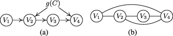
An illustration on how ignoring changes in the causal model may lead to spurious connections by the constraint-based method, (a) The true causal graph (including confounder g(C)). (b) The estimated conditional independence graph on the observed data in the asymptotic case.
To tackle the issue of changing causal models, one may try to find causal models on sliding windows [Calhoun et al., 2014] (for nonstationary data) or in different domains (for data from multiple domains) separately, and then compare them. Improved versions include the online changepoint detection method [Adams and Mackay, 2007], the online undirected graph learning [Talih and Hengartner, 2005], the locally stationary structure tracker algorithm [Kummerfeld and Danks, 2013], and the regime aware learning algorithm to learn a sequence of Bayesian networks (BNs) that model a system with regime changes [Bendtsen, 2016]. Such methods may suffer from high estimation variance due to sample scarcity, large type II errors, and a large number of statistical tests. Some methods aim to estimate the time-varying causal model by making use of certain types of smoothness of the change [Huang et al., 2015], but they do not explicitly locate the changing causal modules. Several methods aim to model time-varying time-delayed causal relations [Xing et al., 2010; Song et al., 2009], which can be reduced to online parameter learning because the direction of the causal relations is given (i.e., the past influences the future). Compared to them, learning changing instantaneous causal relations, with which we are concerned in this paper, is generally more difficult. Moreover, most of these methods assume linear causal models, limiting their applicability to complex problems with nonlinear causal relations.
In contrast, we will develop a nonparametric and computationally efficient causal discovery procedure to discover the causal skeleton and orientations from all data points simultaneously. We term this procedure Constraint-based causal Discovery from Nonstationary/heterogeneous Data (CD-NOD). By analyzing all available data, it efficiently identifies nonstationary causal modules and recovers the causal skeleton. We will also show that distribution shifts actually contain useful information for the purpose of determining causal directions and develop practical algorithms accordingly.
3 CD-NOD Phase 1: Changing Causal Module Detection and Causal Skeleton Estimation
3.1 Assumptions
As already mentioned, we allow changes in causal modules and some of the changes to be related, which may be explained by positing particular types of unobserved confounders. Intuitively, such confounders may refer to some high-level background variables. For instance, for fMRI data, they may be the subject’s attention or some unmeasured background stimuli; for the stock market, they may be related to economic policies. Thus we do not assume causal sufficiency for the set of observed variables. However, we assume that the confounders, if any, can be written as smooth functions of time or domain index. It follows that at each time or in each domain, the values of these confounders are fixed. We call this a pseudo causal sufficiency assumption.
We assume that the observed data are independently but not identically distributed. As a consequence, in this paper we will focus on instantaneous or contemporaneous causal relations; the strength (or model, or even existence) of the causal relations is allowed to change over time or across data sets. We did not explicitly consider time-delayed causal relations and in particular did not engage autoregressive models. However, we note that it is natural to generalize our framework to incorporate time-delayed causal relations in time series, just in the way that constraint-based causal discovery was adapted to handle time-series data (see, e.g., [Chu and Glymour, 2008]).
Denote by the set of such confounders (which may be empty). We further assume that for each Vi the local causal process for Vi can be represented by the following structural equation model (SEM):
| (1) |
where denotes the set of confounders that influence Vi (it is an empty set if there is no confounder behind Vi and any other variable), θi(C) denotes the effective parameters in the model that are also assumed to be functions of C, and εi is a disturbance term that is independent of C and has a non-zero variance (i.e., the model is not deterministic). We also assume that the εi’s are mutually independent.
In this paper we treat C as a random variable, and so there is a joint distribution over . We assume that this distribution is Markov and faithful to the graph resulting from the following additions to G (which, recall, is the causal structure over V): add to G, and for each i, add an arrow from each variable in gi(C) to Vi and add an arrow from θi(C) to Vi. We refer to this augmented graph as Gaug. Obviously G is simply the induced subgraph of Gaug over V.
3.2 Detecting Changing Modules and Recovering Causal Skeleton
In this section we propose a method to detect variables whose causal modules change and infer the skeleton of G. The basic idea is simple: we use the (observed) variable C as a surrogate for the unobserved , or in other words, we take C to capture C-specific information.1 We now show that given the assumptions in 3.1, we can apply conditional independence tests to V ∪ {C} to detect variables with changing modules and recover the skeleton of G. We considered C as a surrogate variable (it itself is not a causal variable, it is always available, and confounders and changing parameters are its functions): by adding only C to the variable set V, the skeleton of G and the changing causal modules can be estimated as if were known. This is achieved by Algorithm 1 and supported by Theorem 1.
The procedure given in Algorithm 1 outputs an undirected graph, UC, that contains C as well as V. In Step 2, whether a variable Vi has a changing module is decided by whether Vi and C are independent conditional on some subset of other variables. The justification for one side of this decision is trivial. If Vi’s module does not change, that means P(Vi | PAi) remains the same for every value of C, and so Vi ⫫ C | PAi. Thus, if Vi and C are not independent conditional on any subset of other variables, Vi’s module changes with C, which is represented by an edge between Vi and C. Conversely, we assume that if Vi’s module changes, which entails that Vi and C are not independent given PAi, then Vi and C are not independent given any other subset of V\{Vi}. If this assumption does not hold, then we only claim to detect some (but not necessarily all) variables with changing modules.
Algorithm 1.
Detection of Changing Modules and Recovery of Causal Skeleton.
|
Step 3 aims to discover the skeleton of the causal structure over V. Its (asymptotic) correctness is justified by the following theorem:
Theorem 1
Given the assumptions made in Section 3.1, for every Vi.,Vj ∈ V, Vi and Vj are not adjacent in G if and only if they are independent conditional on some subset of {Vk| k ≠ i, k ≠ j} ∪ {C}.
Basic idea of the proof
For a complete proof see [Zhang et al., 2015]. The “only if” direction is proven by making use of the weak union property of conditional independence repeatedly, the fact that all gl(c) and θm(C) are deterministic functions of C, some implications of the SEMs Eq. 1, the assumptions in Section 3.1, and the properties of mutual information given in [Madiman, 2008]. The “if” direction is shown based on the faithfulness assumption on Gaug and the fact that is a deterministic function of C.
In the above procedure, it is crucial to use a general, nonparametric conditional independence test, for how variables depend on C is unknown and usually very nonlinear. In this work, we use the kernel-based conditional independence test (KCI-test [Zhang et al., 2011]) to capture the dependence on C in a nonparametric way. By contrast, if we use, for example, tests of vanishing partial correlations, as is widely used in the neuroscience community, the proposed method will not work well.
4 CD-NOD Phase 2: Nonstationarity Helps Determine Causal Direction
We now show that using the additional variable C as a surrogate not only allows us to infer the skeleton of the causal structure, but also facilitates the determination of some causal directions. Let us call those variables that are adjacent to C in the output of Algorithm 1 “C-specific variables”, which are actually the effects of nonstationary causal modules. For each C-specific variable Vk, it is possible to determine the direction of every edge incident to Vk, or in other words, it is possible to infer PAk. Let Vl be any variable adjacent to Vk in the output of Algorithm 1. There are two possible cases to consider:
-
Vl is not adjacent to C. Then C – Vk – Vl forms an unshielded triple. For practical purposes, we can take the direction between C and Vk as C → Vk (though we do not claim C to be a cause in any substantial sense). Then we can use the standard orientation rules for unshielded triples to orient the edge between Vk and Vl [Spirtes et al., 2001; Pearl, 2000]. There are two possible situations:
If Vl and C are independent given a set of variables excluding Vk, then the triple is a V-structure, and we have Vk ←Vl.
Otherwise, if Vl and C are independent given a set of variables including Vk, then the triple is not a V-structure, and we have Vk → Vl.
Vl is also adjacent to C This case is more complex than Case 1, but it is still possible to identify the causal direction between Vk and Vl, based on the principle that P (cause) and P (effect | cause) change independently; a heuristic method is given in Section 4.2.
The procedure in Case 1 contains the methods proposed in [Hoover, 1990; Tian and Pearl, 2001] for causal discovery from changes as special cases, which may also be interpreted as special cases of the principle underlying the method for Case 2: if one of P (cause) and P (effect | cause) changes while the other remains invariant, they are clearly independent.
4.1 Independent Changes of Causal Modules as Generalization of Invariance
There exist methods for causal discovery from changes of multiple data sets [Hoover, 1990; Tian and Pearl, 2001; Peters et al., 2016] by exploiting the property of invariance of causal mechanisms. They used linear models to represent causal mechanism and, as a consequence, the invariance of causal mechanisms can be assessed by checking whether the involved parameters change across data sets or not. Actually, Situation 1.b above provides a nonparametric way to achieve this in light of nonparametric conditional independence test. For any variable Vi and a set of variables S, the conditional distribution P(Vi | S) is invariant across different values of C if and only if
This is exactly the condition under which V1 ⫫ C | S. In words, testing for invariance (or homogeneity) of the conditional distribution is naturally achieved by performing conditional independence test on Vi and C given the variable S, for which there exist off-the-shelf algorithms and implementations. When S is the empty set, this reduces to the test of marginal independence between Vi and C, or the test of homogeneity of P(Vi).
In Situation 1.a, we have the invariance of P (cause) when the causal mechanism, represented by P (effect | cause), changes, which is complementary to the invariance of causal mechanisms. Naturally, both invariance properties above are particular cases of the principle of independent changes of causal modules underlying the method for Case 2: if one of P (cause) and P (effect | cause) changes while the other remains invariant, they are clearly independent. Usually there is no reason why only one of them could change, so the above invariance properties are rather restrictive. The property of independent changes holds in rather generic situations, e.g., when there is no confounder behind cause and effect, or even when there are confounders but the confounders are independent from C. Below we will propose an algorithm for causal direction determination based on independent changes.
4.2 Inference of the Causal Direction between Variables with Changing Modules
We now develop a heuristic method to deal with Case 2 above. For simplicity, let us start with the two-variable case: suppose V1 and V2 are adjacent and are both adjacent to C. We aim to identify the causal direction between them, which, without loss of generality, we assume to be V1 → V2.
Fig. 2(a) shows the case where the involved changing parameters, θ1 (C) and θ2(C) are independent, i.e., P(V1;θ1) and P(V2 | V1; θ2) change independently. (We dropped the argument C in θ1 and θ2 to simplify notations.)
Figure 2.
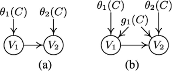
Two possible situations where V1 → V2 and both V1 and V2 are adjacent to C. (a) θ1(C) ⫫ θ2(C). (b) In addition to the changing parameters, there is a confounder g1(C) underlying V1 and V2.
For the reverse direction, one can decompose the joint distribution of (V1, V2) according to
| (2) |
where and are assumed to be sufficient for the corresponding distribution modules P(V2) and P(V1|V2). Generally speaking, and are not independent, because they are determined jointly by both θ1 and θ2. We assume that this is the case, and identify the direction between V1 and V2 based on this assumption.
Now we face two problems. First, how can we compare the dependence between θ1 and θ2 and that between and ? Second, in our nonparametric setting, we do not really have such parameters. How can we compare the dependence based on the given data?
The total contribution (in a way analogous to causal effect; see [Janzing et al., 2013]) from and to (V1, V2) can be measured with mutual information:
| (3) |
where the 2nd and 3rd equalities hold because of the chain rule, the 4th equality because of the relation implied by the sufficiency of for V2, and the 5th equality because the sufficiency of for implies .
Since and are dependent, their individual contributions to (V1, V2) are redundant. Below we calculate the individual contributions. The contribution from to V2 is . The contribution from to V1 has been derived in [Janzing et al., 2013]: , where is an independent copy of (it has the same marginal distribution as but does not depend on ). As a consequence, the dependence (or redundancy) in the contributions from and is
| (4) |
is always non-negative because it is a Kullback-Leibler divergence. One can verify that if , which implies , we have leading to . (Proving the converse is non-trivial, involving some constraint on .)
provides a way to measure the dependence between and . Regarding the second problem mentioned above, since we do not have parametric models, we propose to estimate from the data by:
| (5) |
where 〈·〉 denotes the sample average, is the empirical estimate of P(V1|V2) on all data points, and denotes the sample average of , which is the estimate of P(V1|V2) at each time (or in each domain). In our implementation, we used kernel density estimation (KDE) on all data points to estimate , and used KDE on sliding windows (or in each domain) to estimate . We take the direction for which is smaller to be the causal direction.
If there is a confounder g1(C) underlying V1 and V2, as shown in Fig. 2(b), we conjecture that the above approach still works if the influences from g1(C) are not very strong, for the following reason: for the correct direction, measures the influence from the confounder; for the wrong direction, it measures the influence from the confounder and the dependence in the “parameters” caused by the wrong causal direction. A future line of research is to seek a more rigorous theoretical justification of this method. When there are more than two variables which are connected to C and inter-connected, we try all possible causal structures and choose the one that minimizes the total value, i.e., .
5 Experimental Results
We have applied proposed approaches to a variety of synthetic and real-world data sets. We learned the causal structure by the enhanced constraint-based method (Algorithm 1), and compared it with the SGS algorithm [Spirtes et al., 2001], a constraint-based causal discovery method; for both, we used kernel-based conditional independence test (KCI) [Zhang et al., 2011] with SGS search [Spirtes et al., 1993]. Furthermore, we applied the approaches proposed in Section 4 for further causal direction determination.
5.1 Simulations
A Toy Example
We generated synthetic data according to the SEMs specified in Fig. 3. More specifically, the noise variance of V1, and the causal modules of V4, V5 and V6 are time varying, governed by a sinusoid function of t; for V1 and V4, the time-varying component a(t) is multiplicative, and for V5 and V6, theirs are additive. We tried different periods (w = 5, 10, 20, 30) on the time-varying component a, as well as different sample sizes (N = 600, 1000). The fixed causal mechanisms and g4 are randomly chosen from sinusoid functions, polynomial functions, or hyperbolic tangent functions of Vi’s directed causes, and we set w′ = 200 to ensure the independence between a and b. In each setting, we ran 50 trials. We tested the generated data with proposed enhanced constraint-based method (Algorithm 1, set C to be the time information) and the original constraint-based method. Furthermore, we determined the causal directions by both approaches proposed in Section 4.
Figure 3.
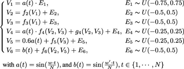
The SEMs according to which we generated the simulated data. The noise variance to V1, and the causal modules of V4 and V5 are time- varying, governed by a; the causal module of V6 are time-varying, governed by b. We tried different periods w, and different sample sizes N.
Fig. 4 shows the False Positive (FP) rate and the False Negative (FN) rate of the discovered causal skeletons with significance level 0.05. It is obvious that compared to the original method, our method effectively reduces the number of spurious edges (represented by FP rate) due to the nonstationarity; specifically, the spurious edges V1 – V4, V1 – V5 and V4 – V5. With the enhanced one, the FN rate only has a slight increase at a small sample size, and keeps the same when N is large. As w increases, both FP and FN stay stable, with a little bit variation; as N increases, the FN rates are reduced with both methods. In addition, with the enhanced constraint-based method we identified those variables, V1, V4, V5 and V6, which have nonstationary causal modules. Furthermore, we successfully identified causal directions by the procedure given in Section 4; specifically, V5 → V6 is identified by the criterion in Section 4.2 with 93.2% accuracy, since a and b change independently, and other causal directions are determined by the procedure given in Case 1. In this simulation, the whole causal DAG is correctly identified. However, with the original method, we only identified two causal directions: 5 → 6 and 2 → 6, and there are spurious edges V1 – V4, V1 – V5 and V4 – V5.
Figure 4.
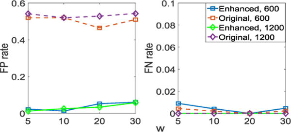
The estimated FP rate and FN rate with w = {5, 10, 20, 30} and N = {600, 1000} by both our enhanced constraint-based method and the original SGS method.
5.2 Real Data
fMRI Hippocampus
This fMRI Hippocampus dataset [Poldrack and Laumann, 2015] contains signals from six separate brain regions: perirhinal cortex (PRC), parahippocampal cortex (PHC), entorhinal cortex (ERC), subiculum (Sub), CA1, and CA3/Dentate Gyrus (CA3) in the resting states on the same person in 64 successive days. We are interested in investigating causal connections between these six regions in the resting states. We used the anatomical connections, for which see [Chris and Neil, 2008], because in theory a direct causal connection between two areas should not exist if there is no anatomical connection between them.
We applied our enhanced constraint-based method on 10 successive days separately, with time information T as an additional variable in the system. We assumed that the underlying causal graph is acyclic, although the anatomical structure gives cycles. We found that our method effectively reduces the FP rate, from 62.9% to 17.1%, compared to the original constraint-based method with SGS search and KCI-test. Here we regard those connections that do not exist in the anatomical structure as spurious; however, with the lack of ground truth, we are not able to compare the FN rate. We found that the causal structure varies across days, but the connections between CA1 and CA3, and between CA1 and SUB are robust, which coincides with the current findings in neuroscience [Song et al., 2015]. In addition, on most data sets the causal graphs we derived are acyclic, which validates the use of constraint-based method. Furthermore, we applied the procedure in Section 4 to infer causal direction. We successfully recovered the following causal directions: CA3 → CA1, CA1 → Sub, Sub → ERC, ERC → CA1 and PRC → BRC, and the accuracy of direction determination is 85.7%.
Breast Tumor Dataset
The breast tumor dataset is from the UCI Machine Learning Depository [Blake and Merz, 1998]. It contains subjects with benign tumor and malignant tumor, 569 subjects each. Ten real-valued features are computed for each cell nucleus, and each feature has three measures: the mean, standard error (SE), and largest value, resulting in 30 features in total. We concatenated the data from benign and malignant subjects and set the additional variable C to be the indicator of the disease (1 for “benign”, and 2 for “malignant”). With our enhanced constraint-based method, we identified the causal connections between features, and we found that only 11 features are directly affected by the tumor type; the 11 features are mean radius, SE of radius, mean perimeter, SE of concave points, worst symmetry, SE of symmetry, worst radius, worst area, mean symmetry, SE of fractal dimension, and mean texture. We then identified the causal orientations between a set of features. Moreover, the features adjacent to C produced the best classification performance: we trained SVM with these 11 features, subsets of these 11 features, random subsets of all features, and all 30 features, and used 10-fold cross-validation (CV) error to assess the classification accuracy. These 11 features give the CV error 0.0246, while the 3 features used in [Street et al., 1993] give 0.0791, and the whole 30 features give 0.0264.
6 Conclusion and Discussions
We have proposed CD-NOD, a framework for causal discovery from nonstationary/heterogeneous data, where causal modules may change over time or across data sets. We assume a pseudo causal sufficiency condition, which states that all confounders can be written as smooth functions of time or the domain index. CD-NOD consists of (1) an enhanced constraint-based method for locating variables with changing generating mechanisms and estimating the skeleton of the causal structure, and (2) a method for causal direction determination that takes advantage of changing distributions.
In future work, we aim to answer the following questions. 1. What if the causal direction also changes? Can we develop a general approach to detect all causal direction changes? 2. To fully determine the causal structure, one might need to combine the proposed framework with other approaches, such as those based on restricted functional causal models. How can this be efficiently accomplished? 3. The issue of distribution shift may decrease the power of statistical (conditional) independence tests. How can we alleviate this effect?
Acknowledgments
Research conducted in this paper was supported by the National Institutes of Health (NIH) under Award Numbers NIH–1R01EB022858-01 FAIN–R01EB022858, NIH–1R01LM012087, and NIH–5U54HG008540-02 FAIN–U54HG008540.
Footnotes
Recall that C may simply be time. Thus in this paper we take time to be a special random variable which follows a uniform distribution over the considered time period, with the corresponding data points evenly sampled at a certain sampling frequency. We realize that this view of time will invite philosophical questions, but for the purpose of this paper, we will set those questions aside. One can regard this stipulation as purely a formal device without substantial implications on time per se.
References
- [Adams and Mackay, 2007].Adams RR, Mackay DJC. Technical report. University of Cambridge; Cambridge, UK: 2007. Bayesian online change point detection. Preprint at http://arxiv.org/abs/0710.3742vl. [Google Scholar]
- [Bendtsen, 2016].Bendtsen M. Regime aware learning. Proceedings of the Eighth International Conference on Probabilistic Graphical Models. 2016:1–12. [Google Scholar]
- [Blake and Merz, 1998].Blake CL, Merz CJ. Nuclear feature extraction for breast tumor diagnosis. UCI repository of machine learning databases. 1998 [Google Scholar]
- [Calhoun et al. 2014].Calhoun VD, Miller R, Pearlson G, Adal T. The chronnectome: Time-varying connectivity networks as the next frontier in fmri data discovery. Neuron. 2014;84:262–274. doi: 10.1016/j.neuron.2014.10.015. [DOI] [PMC free article] [PubMed] [Google Scholar]
- [Chris and Neil, 2008].Chris MB, Neil B. The hippocampus and memory: insights from spatial processing. Nature Reviews Neuroscience. 2008;9:182–194. doi: 10.1038/nrn2335. [DOI] [PubMed] [Google Scholar]
- [Chu and Glymour, 2008].Chu T, Glymour C. Search for additive nonlinear time series causal models. Journal of Machine Learning Research. 2008;9:967–991. [Google Scholar]
- [Havlicek et al. 2011].Havlicek M, Friston KJ, Jan J, Brazdil M, Calhoun VD. Dynamic modeling of neuronal responses in fMRI using cubature kalman filtering. Neuroimage. 2011;56:2109–2128. doi: 10.1016/j.neuroimage.2011.03.005. [DOI] [PMC free article] [PubMed] [Google Scholar]
- [Hoover, 1990].Hoover K. The logic of causal inference. Economics and Philosophy. 1990;6:207–234. [Google Scholar]
- [Hoyer et al. 2009].Hoyer PO, Janzing D, Mooji J, Peters J, Schölkopf B. Nonlinear causal discovery with additive noise models. NIPS. 2009;21 [Google Scholar]
- [Huang et al. 2015].Huang B, Zhang K, Schölkopf B. Prof IJCAI 2015. Buenos, Argentina: 2015. Identification of time-dependent causal model: A gaussian process treatment; pp. 3561–3568. [Google Scholar]
- [Janzing et al. 2013].Janzing D, Balduzzi D, Grosse-Wentrup M, Schölkopf B. Quantifying causal influences. Ann Statist. 2013;41:2324–2358. [Google Scholar]
- [Kummerfeld and Danks, 2013].Kummerfeld E, Danks D. Advances in neural information processing systems. Vol. 26. La Jolla, CA: 2013. Tracking time-varying graphical structure. [Google Scholar]
- [Madiman, 2008].Madiman M. On the entropy of sums. Proceedings of IEEE Information Theory Workshop (ITW’08) 2008:303–307. [Google Scholar]
- [Pearl, 2000].Pearl J. Causality: Models, Reasoning, and Inference. Cambridge University Press; Cambridge: 2000. [Google Scholar]
- [Peters et al. 2016].Peters J, Bühlmann P, Meinshausen N. Causal inference using invariant prediction: identification and confidence intervals. Journal of the Royal Statistical Society: Series B. 2016 [Google Scholar]
- [Poldrack and Laumann, 2015].Poldrack R, Laumann T. 2015 https://openfmri.org/dataset/ds000031/
- [Shimizu et al. 2006].Shimizu S, Hoyer PO, Hyvärinen A, Kerminen AJ. A linear non-Gaussian acyclic model for causal discovery. Journal of Machine Learning Research. 2006;7:2003–2030. [Google Scholar]
- [Song et al. 2009].Song L, Kolar M, Xing E. Time-varying dynamic Bayesian networks. NIPS. 2009;23 [Google Scholar]
- [Song et al. 2015].Song D, Hsiao MC, Opris I, Hampson RE, Marmarelis VZ, Gerhardt GA, Deadwyler SA, Berger TW. Hippocampal microcircuits, functional connectivity, and prostheses. Recent Advances On the Modular Organization of the Cortex. 2015:385–405. [Google Scholar]
- [Spirtes et al. 1993].Spirtes P, Glymour C, Schemes R. Causation, Prediction, and Search. Spring-Verlag Lectures in Statistics. 1993 [Google Scholar]
- [Spirtes et al. 2001].Spirtes P, Glymour C, Schemes R. Causation, Prediction, and Search. 2nd. MIT Press; Cambridge, MA: 2001. [Google Scholar]
- [Street et al. 1993].Street WN, Wolberg WH, Mangasarian OL. Nuclear feature extraction for breast tumor diagnosis. IS &T/SPIE’s Symposium on Electronic Imaging: Science and Technology International Society for Optics and Photonics. 1993 [Google Scholar]
- [Talih and Hengartner, 2005].Talih M, Hengartner N. Structural learning with time-varying components: Tracking the cross-section of financial time series. Journal of the Royal Statistical Society - Series B. 2005;67(3):321–341. [Google Scholar]
- [Tian and Pearl, 2001].Tian J, Pearl J. Causal discovery from changes: a bayesian approach. Proc UAI 2001. 2001:512–521. [Google Scholar]
- [Xing et al. 2010].Xing EP, Fu W, Song L. A state-space mixed membership blockmodel for dynamic network tomography. Annals of Applied Statistics. 2010;4(2):535–566. [Google Scholar]
- [Zhang and Chan, 2006].Zhang K, Chan L. Extensions of ICA for causality discovery in the hong kong stock market. Proc 13th International Conference on Neural Information Processing (ICONIP 2006) 2006 [Google Scholar]
- [Zhang and Hyvärinen, 2009a].Zhang K, Hyvärinen A. ECML PKDD 2009. Bled, Slovenia: 2009. Acyclic causality discovery with additive noise: An information-theoretical perspective. [Google Scholar]
- [Zhang and Hyvärinen, 2009b].Zhang K, Hyvärinen A. On the identifiability of the post-nonlinear causal model; Proceedings of the 25th Conference on Uncertainty in Artificial Intelligence; Montreal, Canada. 2009. [Google Scholar]
- [Zhang et al. 2011].Zhang K, Peters J, Janzing D, Schölkopf B. Kernel-based conditional independence test and application in causal discovery; Proceedings of the 27th Conference on Uncertainty in Artificial Intelligence (UAI 2011); Barcelona, Spain. 2011. [Google Scholar]
- [Zhang et al. 2015].Zhang K, Huang B, Zhang J, Schölkopf B, Glymour C. Discovery and visualization of nonstationary causal models. 2015 available at https://arxiv.org/abs/1509.08056.