On the Adjustment for Covariates in Genetic Association Analysis: A Novel, Simple Principle to Infer Direct Causal Effects

Abstract

In genetic association studies, different complex phenotypes are often associated with the same marker. Such associations can be indicative of pleiotropy (i.e. common genetic causes), of indirect genetic effects via one of these phenotypes, or can be solely attributable to non-genetic/environmental links between the traits. To identify the phenotypes with the inducing genetic association, statistical methodology is needed that is able to distinguish between the different causes of the genetic associations. Here, we propose a simple, general adjustment principle that can be incorporated into many standard genetic association tests which are then able to infer whether an SNP has a direct biological influence on a given trait other than through the SNP’s influence on another correlated phenotype. Using simulation studies, we show that, in the presence of a non-marker related link between phenotypes, standard association tests without the proposed adjustment can be biased. In contrast to that, the proposed methodology remains unbiased. Its achieved power levels are identical to those of standard adjustment methods, making the adjustment principle universally applicable in genetic association studies. The principle is illustrated by an application to three genome-wide association analyses.

INTRODUCTION

It is a well-studied phenomenon that the findings of genetic association studies can be confounded and biased by genetic and/or phenotypic heterogeneity which is not accounted for in the statistical analysis. Consequently, much effort has been devoted to the development of statistical analysis techniques that minimize the impact of such effects, in particular to approaches to control for population admixture and stratification [Pritchard and Rosenberg, 1999; Devlin and Roeder, 1999; Price et al., 2006; Epstein et al., 2007]. However, relatively little is known and understood about situations in which a genetic association with the disease phenotype is confounded by an association between the same marker and another phenotype [Smoller et al., 2000; Robins et al., 2001]. If the two phenotypes are linked other than just through the tested marker locus, a true association with one phenotype can cause an association between the same marker locus and the other phenotype, despite the lack of an independent, direct genetic effect on that phenotype and thus even in the absence of pleiotropy. Such situations can be encountered in genome-wide association studies (GWAS), in pathway analysis of candidate genes, and in association studies that incorporate genomic information into the association analysis.

Recent GWAS revealed strong associations between the same SNPs and different phenotypes [Hung et al., 2008; Amos et al., Thorgeirsson et al., 2008; Bierut et al., 2007; Frayling et al., 2007]. Scans for lung cancer showed highly significant associations with a set of SNPs [Hung et al., 2008; Amos et al.]. In an independent study, associations between the same SNPs and smoking behavioral phenotypes reached also genome-wide significance [Thorgeirsson et al., 2008]. Given the strong non-genetic link between both phenotypes, lung cancer and smoking behavior, there is currently no conclusive evidence whether the identified SNPs describe a lung cancer gene or a smoking-behavior gene [Chanock and Hunter, 2008]. A similar situation occurred in GWAS for obesity [Frayling et al., 2007; Scuteri et al., 2007], in which the strongest association for body-mass index is observed for an SNP in the FTO gene. The SNP was also identified as one of the “top hits” by a GWAS for smoking-behavior [Bierut et al., 2007]. Again, given the non-genetic link between both phenotypes [Li et al., 2003; Zimlichman et al., 2005], the identification of the causative association is not straightforward. In view of these quandaries, our goal in this article is to infer whether a given marker is (causally) associated with the disease phenotype other than through its association with a secondary, intermediate phenotype.

A standard epidemiological approach to remove the effect of a secondary phenotype/covariate on the target phenotype is to regress the target phenotype on the secondary phenotype (and possibly also other influencing factors/covariates) and to use the corresponding residuals as the phenotype of interest in the association analysis. An alternative, common approach is to test whether the SNP is associated with the target phenotype after adjusting for the other phenotype. Both approaches are also used to reduce variability and can be fallible. For the first approach, this is partly because by removing the association between both phenotypes (via residuals), one risks to remove also part of the effect of the SNP on the target phenotype (see the section “The Limitation of Standard Analysis Approaches for the Detection of Direct Genetic Effects”). For the second approach this is because adjustment for phenotypes, or more generally covariates, is only valid under the assumption that the influencing factors/covariates are not associated with the marker locus [Rosenbaum, 1984; Cole and Hernan, 2002]. In particular in the context of GWAS which interrogate the entire human genome, this assumption is generally untenable, e.g., the adjustment for physiological factors with relatively high heritability such as height [Carmichael and McGue, 1995; Hirschhorn et al., 2001].

A conceptually different situation is encountered in genetic association studies that incorporate genomic data, e.g., expression profiles [Schadt et al., 2005]. Here, associations between the same marker and both traits, the expression profile and the disease phenotype of interest, can be especially informative. If one is able to conclude that the observed association between the marker and the disease phenotype is caused by the association with the expression profile, this provides stronger evidence for the validity of a finding than an association with just the disease phenotype.

Common to all scenarios that were discussed above, is that the non-marker related link between the different phenotypes can bias the results of the association analysis. Specifically, an association between a marker and a particular phenotype can cause an apparent association between the same marker and another phenotype if there is a causal link between both phenotypes. In order to identify the true genetic pathways of complex diseases, it will be crucial to have the ability to distinguish whether an observed genetic association with a particular phenotype is attributable to a link with another phenotype that is itself associated with the marker, or whether the observed association is independent of that, thus indicating a direct causal genetic relationship between the marker locus and the examined phenotype.

To address this problem, we propose a simple, general principle to adjust the phenotype of interest for a potential association between the examined marker and another, related phenotype. Using causal inference methodology, we develop an adjustment approach that is applicable to both binary and quantitative traits, and that is computationally simple. The adjusted phenotype can be incorporated into many standard genetic association tests which then test for a direct genetic effect between the phenotype of interest and the marker (other than through the given intermediate phenotype). The principle is outlined first by application to quantitative phenotypes both in population-based designs and in family-based studies. The integration of the approach for binary traits, e.g., association studies of unrelated cases and controls in cohort studies, is also discussed.

Using both theoretical considerations and simulation studies, we demonstrate that, in the presence of a non-genetic link between the phenotype of interest and the other phenotype, association tests with adjustment procedures that are based on intuitive regression approaches can be biased and provide incorrect results. Further, the simulation studies show that the proposed adjustment principle is sufficiently powered to detect direct genetic effects for realistic sample sizes. When the adjustment principle is applied in situations of no relationship between both phenotypes, the adjusted association test still achieves power levels that are virtually identical to those of standard regression approaches, making the proposed principle a generally applicable approach for covariate-adjustment in genetic association studies.

As a real data example, we present results from a 100 k-scan in the Framingham Heart Study that suggested an association between an SNP and two phenotypes, FEV₁ and BMI, which was detected using a standard regression-based covariate adjustment. The application of the proposed adjustment method suggests that the “true” effect of this SNP may have fully originated from its association with BMI. This conclusion is then confirmed by replication analysis in two independent GWAs, the CAMP study [C. A. M. P. R. Group, 1999] and the British Birth Cohort.

THE LIMITATION OF STANDARD ANALYSIS APPROACHES FOR THE DETECTION OF DIRECT GENETIC EFFECTS

Suppose that in the study of interest, n subjects have been genotyped at a specified marker locus and their coded genotype is denoted by X_i, i = 1, …, n. If the selected sample is a family-based study, we further assume that additional genotype data on other family members are available so that the expected marker score, E(X_i|S_i), can be computed conditional on Mendelian transmissions. When parental data are available, the variable S_i denotes the parental genotypes; otherwise it represents the sufficient statistic by Rabinowitz and Laird [Rabinowitz and Laird, 2000].

Two phenotypes, K_i and ϒ_i, have been recorded for the ith subject, where ϒ_i is the target phenotype for the primary association analysis of the study. The phenotype K_i is of secondary interest in the study, e.g., an endo/intermediate phenotype or covariate for the target phenotype ϒ_i. Both phenotypes may be influenced by shared, non-genetic confounding variables and may thus be correlated. The phenotype K_i has been tested for association with the marker locus, and a significant association has been observed. Now, given the established association between the marker locus and the secondary phenotype K_i, our goal is to test for an association between the target phenotype ϒ_i and the marker locus that cannot be explained by the existing genetic association with phenotype K_i and the correlation between both phenotypes.

To understand the problems of standard intuitive regression approaches when they are applied to adjust for confounding in the context of genetic association studies, we use causal diagrams [Pearl, 1995; Robins, 2001]. These postulate the causal relationships between all measurements of interest by means of directed arrows, as in Figure 1. If the study of interest has a family-based design, the variable S encodes the parental genotypes. For study designs with unrelated probands, S denotes measured factors inducing population admixture. Further, L is a collection of measured prognostic factors for the secondary phenotype K. As we will see later, the presence of S allows for the association between the marker X and both phenotypes to be confounded by measured factors. Likewise, the presence of L allows for the association between both phenotypes to be confounded by measured factors.

Fig. 1.

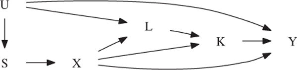
Causal diagram illustrating the confounding of the genetic association between the target phenotype ϒ and the marker locus X. The variable K denotes the intermediate phenotype, X the marker score, and S the parental genotypes (in the case of a family-based study, and measured factors inducing population admixture otherwise). U denotes a collection of unmeasured factors that allow for confounding due to population admixture and of common risk factors of both phenotypes.

For the diagram in Figure 1 to infer causal genetic effects, it must satisfy the following two basic assumptions:

1. The absence of an arrow between any two variables A and B encodes the assumption that A exercises no direct causal effect on B. Figure 1, thus, postulates that the common confounders S and L cannot affect the target phenotype ϒ other than by affecting the marker X and phenotype K, respectively. We will relax this restriction in the Appendix. Figure 1 further postulates that the target phenotype ϒ is affected by the intermediate phenotype K and not the other way around. We will elaborate on this restriction in the “Discussion” section.

2. The diagram includes all variables that jointly affect any two variables in the diagram. Figure 1, thus, postulates that all risk factors for the secondary phenotype K, which are also associated with the target phenotype ϒ, have been measured and are contained in L. Note that, to add realism, we allow for the relationship between the primary phenotype and the confounding factors L and S to be partly non-causal by means of the unmeasured common cause U.

Two variables in a causal diagram may be statistically associated along all paths that have no converging arrows. That is, they may be associated along all unbroken sequences of edges between those two variables, disregarding the direction of the arrows, in which there are no so-called colliders (i.e., nodes in which two arrows converge, or, point to each other) [Pearl, 1995; Robins, 2001]. Specifically, the genotype X and primary phenotype ϒ in Figure 1 may be associated for three reasons: (1) because of a direct genetic effect (i.e., along the path X → ϒ); (2) because of an indirect genetic effect (i.e., along the paths X → K → ϒ and X → L → K → ϒ) and (3) because of population admixture (i.e., along the paths X ← S ← U → ϒ and X ← S ← U → L → K → ϒ). Importantly, note that when the target phenotype ϒ is not directly genetically affected, then (in the absence of population admixture) no association can be detected between the genotype and the target phenotype, unless there is a causal link between both phenotypes ϒ and K (i.e., unless K causally affects ϒ). A non-causal relationship between both phenotypes will not induce an association between the genotype and the target phenotype because the converging arrows along the paths X → K ← L ← U → ϒ and X → L ← U → ϒ transmit no association.

We will now use the causal diagram in Figure 1 to gain insight into the lack of validity of common regression approaches to test the hypothesis whether the SNP directly affects the target phenotype ϒ other than through the intermediate phenotype K. A first common approach is to eliminate the effects of the established association with the other phenotype K_i by regressing the target phenotype ϒ_i on K_i and using the residuals of ϒ_i as the new phenotype in the association test. This approach has the disadvantage that the residuals remove the overall association between both phenotypes, which mixes the effect of the intermediate phenotype on the target trait (i.e., along the path K → ϒ), with spurious (i.e., non-causal) associations through the SNP X (i.e., along the paths K(← L) ← X → ϒ and K(← L) ← X ← S ← U → ϒ) and by spurious association other than through the SNP X (i.e., along the path K ← L ← U → ϒ). By not solely removing the causal effect of the intermediate phenotype on the target trait, these residuals may be associated with the SNP, even when it has no influence on the target trait. In particular, suppose that the SNP directly influences K, but not ϒ, and that K has no effect on ϒ. Then the SNP has neither a direct, nor an indirect effect on ϒ. Nonetheless, the residual, say ϒ − γK, will have γ ≠ 0 because ϒ is spuriously associated with K along the path K ← L ← U → ϒ, and will be associated with the SNP by the fact that the phenotype K is influenced by it.

An alternative common approach to test the hypothesis that the SNP has a direct influence on the target phenotype other than through the phenotype K, is to measure the association between the genotype X and the target phenotype ϒ conditional on K (e.g., by regressing ϒ on X and K). To appreciate the impact of such adjustment for the phenotype K, note that the adjustment for a variable K on a path between two variables X and ϒ in the causal diagram blocks (i.e., removes) the association between those variables along that path [Pearl, 1995; Robins, 2001]. This is true except when K is a collider or a descendant of a collider along that path, in which case an association is induced [Pearl, 1995; Robins, 2001]. Stratification of the analysis on the secondary phenotype K, thus, removes the indirect effect of the marker X on the target phenotype ϒ by blocking the path X → K → ϒ, but at the same time induces a spurious association along the path X → K ← L ← U → ϒ because the phenotype K is a collider along that path. Additional adjustment for the confounders L blocks this association, but induces a new, non-causal association along the path X → L ← U → ϒ, unless the confounders L are not affected by the marker X.

In summary, traditional approaches for estimating/testing direct genetic effects, either based on an analysis of residuals or based on ordinary regression adjustment, may yield biased inferences for direct genetic effects whenever the association between the intermediate and target phenotype is confounded by a non-genetic link between the two phenotypes. Traditional regression adjustment for measured confounders remains problematic when (some of) these confounders are themselves influenced by the target SNP. We will later verify these theoretical considerations by simulation experiments. In the next section, we propose an alternative adjustment principle which is valid even when confounders/covariates in a genetic association analysis are genetically affected by the same genetic locus.

A GENERAL PRINCIPLE TO TEST FOR CAUSAL DIRECT GENETIC EFFECTS

For simplicity, we illustrate the principle first for the association analysis of quantitative traits, either in population-based designs or in family-based designs. For both scenarios, i.e., population-based studies and family-based studies, we assume that the selected association test T (e.g., a standard score test, Wald test or likelihood ratio test) has the general form

$$T={\displaystyle \sum _{i=1}^n{T}_i,}$$ (1)

where T_i denotes the contribution of the ith subject to the test statistic. To keep the notation simple and without loss of generality, we assume that, under the null hypothesis of no association between the selected phenotype and the marker locus, the expected value of the test statistic T is 0, i.e., E(T) = 0.

In order to derive a valid association test for the direct association between phenotype ϒ and the marker locus that is not influenced by the existing association between the phenotype K and the same disease-specific locus (DSL), we have to assess/estimate the effect of K_i on the target phenotype ϒ_i. Inferring this requires knowledge on common risk factors of both phenotypes, as this allows for disentangling a spurious association between both traits from a real effect. A test for a direct genetic effect between the DSL and the target-phenotype ϒ_i will, therefore, require measurements on all shared, non-genetic factors of both phenotypes. As we will see in the simulation study, this assumption applies only to the major non-genetic factors of both phenotypes, which are often known.

For simplicity, we assume here that the target phenotypes ϒ_i and the phenotype K_i share a common risk factor L_i. Then, in a population-based study, the following linear model can be used to assess how the phenotype K_i influences the target phenotype ϒ_i

$$E({\mathit{\Upsilon }}_i)={\gamma }_0+{\gamma }_1{K}_i+{\gamma }_2{X}_i+{\gamma }_3{L}_i.$$ (2)

In a family-based study, the expected marker-score, E(X_i|S_i), would be added to the model to maintain robustness against population admixture (see the Appendix), i.e.,

$$E(Y_i)={\gamma }_0+{\gamma }_1{K}_i+{\gamma }_2{X}_i+{\gamma }_3{L}_i+{\gamma }_{4}E(X_i|S_i).$$ (3)

In both equations, γ₀,γ₁,γ₂,γ₃ and γ₄ denote the mean parameters. Importantly, note that models (2) and (3) include the offspring genotype X_i as well as the common risk factor L_i of both phenotypes, in order to ensure that g₁ represents the true effect of K_i on ϒ_i and no spurious association. This will guarantee later during the computation of the adjusted phenotypes/residuals that only the effect of K_i is removed from the target phenotype, but a potential direct association between ϒ_i and the marker locus is maintained. Indeed, it follows upon applying the principles outlined in the previous section to the causal diagram in Figure 1, that adjustment for X_i, L_i and S_i blocks all non-causal paths from K_i to ϒ_i and thus reveals the causal effect of K_i on ϒ_i.

Using ordinary least squares to estimate all parameters in model (2) or (3), the target-phenotype ϒ_i can be adjusted for just the effect that the phenotype K_i has on the target phenotype ϒ_i,

$${\stackrel{\sim }{\mathit{\Upsilon }}}_i={\mathit{\Upsilon }}_i-\overline{y}-{\widehat{\gamma }}_1(K_i-\overline{k}),$$ (4)

where ${\widehat{\gamma }}_1$ is the ordinary least squares estimate for g₁ in model (2) or (3). The quantities $\overline{y}$ and $\overline{k}$ are the observed phenotypic means of ϒ and K, respectively, in the sample. The phenotype adjustment (4) here deliberately only involves the other phenotype K_i, but not the shared risk factor L_i. Although this may seem counterintuitive and contrary to standard practice, including factors such as L_i in the phenotypic adjustment would introduce bias if the common risk factor L_i is itself associated with the DSL. As shown in the Appendix, if the residuals ${\stackrel{\sim }{\mathit{\Upsilon }}}_i$ are computed based on the adjustment formula (4), this problem is avoided.

Using now the adjusted phenotype ${\stackrel{\sim }{\mathit{\Upsilon }}}_i$ as the target phenotype, we can construct standard association tests for quantitative traits in either population-based or family-based designs. For example, in a population-based setting, the adjusted phenotype ${\stackrel{\sim }{\mathit{\Upsilon }}}_i$ can be tested for association with a standard regression approach, e.g. each subject’s contribution to the test statistic is given by

$$T_i=X_i{\stackrel{\sim }{\mathit{\Upsilon }}}_i.$$ (5)

For family-based studies, we can construct an association test based on a standard FBAT statistic [Laird et al., 2000] by defining the contribution of each offspring to be

$$T_i=\{X_i-E(X_i|S_i)\}{\stackrel{\sim }{\mathit{\Upsilon }}}_i.$$ (6)

Both association tests, (5) and (6), will then test for a direct association between the DSL and the target-phenotype ϒ_i (where “direct” means “other than through its association with the phenotype K_i”). More generally, as we show in the Appendix, any association test statistic T which is linear in the phenotype and which selects the adjusted phenotype ${\stackrel{\sim }{\mathit{\Upsilon }}}_i$ as the target phenotype will provide a valid and robust test for the null hypothesis that there is no direct effect between the target phenotype ϒ_i and the DSL, i.e., that the apparent association between the target phenotype ϒ_i and the DSL is solely attributable to the established association between the DSL and the other phenotype K_i. Under this condition, the expected value of the test statistic T will be zero, E(T) = 0 when T is computed based on the adjusted phenotype (defined in equation (4)). Further, for family-based tests, we show that, under the null hypothesis of no direct effect, the modified FBAT-statistic (6) remains robust against confounding due to population admixture, provided that population admixture on both phenotypes is w.r.t. unrelated causes (since there would otherwise exist unmeasured common causes of both phenotypes).

The proposed phenotype adjustment (equation (4)) of the association test T for a direct genetic effect includes a parameter estimate for γ₁ that is obtained by fitting model (2) or (3). Since the imprecision of the estimate for g₁ must be acknowledged in the computation of the asymptotic variance of the test statistic, the standard variance of the selected association test is not applicable here anymore. In the Appendix, we show that the standardized association test statistic for the adjusted phenotype T²/(nΣ) follows a χ² distribution with 1 degree of freedom under the null hypothesis of no direct effect, where the variance of the test statistic, Σ, is given by

$$\sum =\mathrm{\text{Var}}({\stackrel{\sim }{T}}_i)$$

with

$${\stackrel{\sim }{T}}_i=T_i-E[{T^{\prime }}_i{K}_i]\frac{(K_i-{\mu }_K^{(i)})}{{\sigma }_K^2}{\epsilon }_i,$$

where T_i denotes the contribution of the i th subject to the association test statistic and T′_i the first order derivative of T_i w.r.t. ${\stackrel{\sim }{\mathit{\Upsilon }}}_i$ (e.g., for population-based tests, we have T_i = X_i in (5) and, for family-based tests, T_i = X_i – E(X_i|S_i)in (6)). The variable ε_i is the residual in model (2) or (3). In population-based designs, the parameters μ_K and ${\sigma }_K^2$ are obtained by fitting a linear regression for K_i with the covariates L_i and X_i. For family-based studies, the covariate E(X|S_i) has to be included well. The predicted value for K_i is then defined by ${\mu }_K^{(i)}=E(K|L_i,X_i)$ or by ${\mu }_K^{(i)}=E(K|L_i,E(X|S_i))$. The residual variance in the model is denoted by ${\sigma }_K^2$.

When the phenotype of interest ϒ_i is dichotomous, e.g., affection status, the proposed adjustment can be extended provided that a relative risk model and a log-link function is assumed. The technical details are discussed in the Appendix.

DATA ANALYSIS: AN APPLICATION TO THE FRAMINGHAM HEART STUDY, THE BRITISH BIRTH COHORT AND THE CAMP STUDY

We evaluated the practical relevance of the proposed adjustment principle by an application to three GWAS: a 100 K Affymetrix scan in the family-plates of the Framing-ham Heart Study (1,400 probands) [Herbert et al., 2006], a 550 K Illumina scan in the British Birth Cohort (genotype data on 1,430 probands, http://www.b58cgene.sgul.ac.uk/) and a 550 K Illumina scan in 440 trios of the CAMP study [C. A. M. P. R. Group, 1999]. As target phenotype, we selected the lung-function measurement FEV1, which was available in all three studies. Since the three studies were genotyped on different platforms (the Framingham Heart Study on 100 K Affymetrix, the British Birth Cohort and CAMP on Illumina 550 K), we selected the 32,121 SNPs for the analysis that are common among both platforms.

As the first step, we analyzed FEV1 at exam 1 in the family-plates of the Framingham Heart Study. Using a standard regression approach, we adjusted FEV1 for height [Bierut et al., 2007], gender, weight and age, and then used the residuals as the target phenotype in the analysis. All statistical analysis was conducted under an additive mode of inheritance. Since the Framingham Heart Study is a family-based study, we applied the weighted Bonferroni-testing strategy by Ionita-Laza et al. [2007] [Van Steen et al., 2005; Laird and Lange, 2006]. Based on the conditional mean model approach [Lange et al., 2003], the testing strategy evaluates the evidence for association at a population level and then estimates the conditional power of the FBAT-statistic for each marker in the first step. In the second step of the testing strategy, FBAT-statistics are computed for all markers. Their significance is assessed based on individually adjusted α-levels that maintain the overall type-1 error and that are weighted based on the conditional power estimate for the corresponding marker.

When the weighted Bonferroni approach was applied to the 32,121 SNPs that are on both genotyping platforms, none of the SNPs reached genome-wide significance. However, the SNP (rs2415815) with the highest conditional power estimate had an unadjusted FBAT P-value of 0.023, warranting additional analysis. When the covariates were tested for association with rs2415815, an association with weight was observed (P-value of 0.0054 for FBAT adjusted for age and gender). Both associations between the SNP and the two phenotypes were then verified in the CAMP study and the British Birth Cohort (Table I). For weight, SNP rs2415815 has nominal significant P-values in CAMP and the British Birth Cohort (measured as BMI), while the association tests with FEV1 are not significant in either studies. Given the established non-genetic link between FEV1 and weight [Oliveti et al., 2006; Yuan et al., 2002; Gessner and Chimonas, 2007; Sin et al., 2004; Demissie et al., 1998; Taveras et al., 2006; Camargo Jr et al., 1999] and the inconsistent replication results, both phenotypes, FEV1 and weight, were re-analyzed with the proposed adjustment procedure in CAMP and FHS. For the British Birth Cohort, we did not have access to the raw data and the proposed adjustment could not be computed.

TABLE I.

Association with rs2415815 in the Framingham Heart Study (FHS), the CAMP Study and the British Birth Cohort (BBC): overall association (overall), direct association based on standard residuals adjusting for K (direct-standard) and based on proposed residuals (direct-proposal)

			FHS			CAMP		BBC
Target phenotype ϒ	Intermediate phenotype K	Adjustment	Effect	95% CI	P	Effect	95% CI	P	P
FEV1	Weight	Overall			0.038			0.59	0.44
		Direct-standard	−0.35	−2.38 to 1.68	0.74	1.78	−1.17 to 4.72	0.24
		Direct-proposal	−1.34	−2.94 to 0.27	0.10	−0.45	−3.57 to 2.77	0.78
Weight	FEV1	Overall			0.0054			0.00053	0.0445*
		Direct-standard	−1.20	−2.22 to −0.18	0.021	−0.14	−0.26 to −0.0064	0.040
		Direct-proposal	−1.34	−2.32 to −0.35	0.0087	−0.16	−0.27 to −0.055	0.0033

^*Measured as BMI.

The lung-function measurement FEV1 (i.e., ϒ) was adjusted for its covariates gender, age and height (i.e., L) and for a potential association with the SNP (i.e., X), the expected marker score given the parental genotypes (i.e., E(X|S)) and weight (i.e., K) (see Fig. 1). Using the estimated association with body weight of 0.118 (SE 0.050) in the FHS, an adjusted phenotype was calculated as $\mathit{\Upsilon }-\overline{y}-0.118(K-\overline{k})$. Based on this adjusted phenotype, the FBAT-statistics in FHS (and similarly in CAMP) were re-calculated (Table I). The association tests for FEV1 in FHS and in CAMP were no longer significant (1), suggesting a 1.34 (95% confidence interval: −2.94–0.27) unit reduction in expected FEV1 per unit increase in marker score when body weight is controlled at a fixed level for all. Because we cannot rule out the possibility of causal effects of FEV1 on body weight, we repeated the analysis with the roles of FEV1 and body weight reversed. In these analyses, the associations with weight remained significant. In the Appendix we show that, if the causal diagram underlying this analysis is wrong because body weight affects FEV1 and not vice versa, then the resulting test can be interpreted as an overall test for genetic association with body weight provided that FEV1 is not directly affected by the studied SNP.

In summary, our results suggest that the originally observed association with FEV1 in the FHS was likely attributable to the association with weight. More precisely, we found no evidence of a direct genetic effect of rs2415815 on FEV1 other than through its association with weight.

SIMULATION STUDY

Using simulation studies, we assess the type-1 error, the power and the robustness of the new approach and compare it to the two standard approaches earlier described. The new principle is evaluated under various conditions, including scenarios in which there are unmeasured risk factors that are common for both phenotypes and that are not included in the adjustment formula. In all simulations, we focus on quantitative traits and assume that there is no ascertainment condition. A sample size of 1,000 probands is selected. All simulation results that are presented in this article are based on 5,000 replicates. With the data analysis example in the Framingham Heart Study in mind, the phenotype of interest ϒ is simulated so that it resembles the FEV1 phenotype in that application. The second phenotype K is weight and the set of common confounding variables is given by height and age, which are denoted by L and S, respectively. First the genotype data are generated by drawing from a Binomial distribution with the specified marker allele frequency. Using the genotype data, all phenotypic variables are simulated from normal distributions under the causal diagrams of Figure 2, with phenotypic means and variances that were observed in the application to the Framingham Heart Study. In addition, unless otherwise specified, effect sizes were also chosen to match the data application.

Fig. 2.

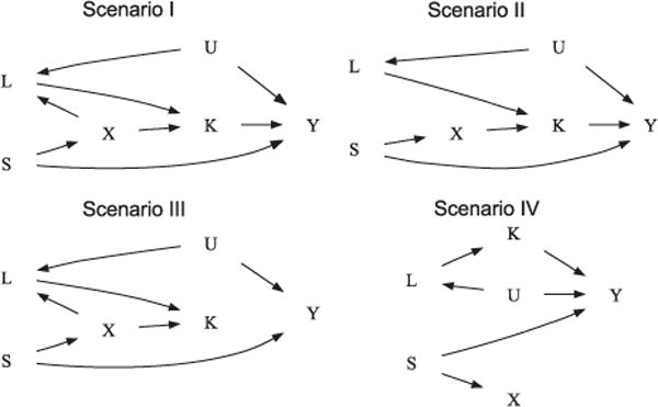
Causal diagrams illustrating the data generating mechanism under simulation scenarios I–IV.

Five tests are evaluated each time. The first two test the association between the target phenotype ϒ and the marker locus with standard Wald tests that are applied to the adjusted phenotypic residuals, where the residuals are obtained from linear regressions adjusting for either (S, K) or (S, K, L). The next two test this association with standard Wald tests that are applied to the phenotype itself, adjusting for either (S, K) or (S, K, L). Finally, we evaluate the proposed adjustment principle.

EMPIRICAL SIGNIFICANCE LEVEL

The first set of simulation studies is conducted under the null hypothesis of no direct genetic effect on the target phenotype ϒ. In order to assess the robustness of the adjustment principle against spurious associations, we consider the following scenarios corresponding to the causal diagrams in Figure 2:

• In the first scenario, we assume that there is a direct genetic effect of the marker on the intermediate phenotype K and on the common covariate L. Each genetic effect has a locus specific heritability of 1%. The intermediate phenotype K explains 1% of the phenotypic variation in ϒ, creating an association between the SNP and ϒ.

• In the second simulation experiment, the first scenario is modified so that there is no genetic effect on the confounder L, but the genetic association with the intermediate phenotype K is still present. Under these conditions, a standard adjustment for the covariate L will provide correct results for the Wald test.

• The third simulation experiment varies from the first scenario with respect to the association between the phenotypes ϒ and K. While the common confounder L is still associated with the marker locus in the third scenario, there is no link anymore between the intermediate phenotype K and the target phenotype ϒ, making an adjustment for the intermediate phenotype K in the association analysis unnecessary.

• In the fourth simulation experiment, the second scenario is modified so that there is also no genetic effect on the intermediate phenotype K.

For a variety of allele frequencies, the estimated nominal significance levels are shown in Table II for the five different tests (performed at the 5% significance level), along with the empirical bias and standard error of the proposed direct effect estimate.

TABLE II.

Empirical type-1 errors at 5% significance level of Wald tests for genetic effects, (a) based on residuals adjusted for (S, K, L), (S, K), (b) directly adjusted for (S, K, L), (S, K) and (c) adjusted with the proposed adjustment principle (D, along with bias and standard error of the direct effect size estimate)

		Wald test on residuals adjusted for		Wald test on trait adjusted for		Proposed adjustment principle
Scenario	Freq	(S, K, L)	(S, K)	(S, K, L)	(S, K)	(D)	Bias × 103	SE
I	0.05	0.080	0.150	0.044	0.134	0.051	−2.05	0.43
	0.1	0.085	0.079	0.065	0.075	0.047	3.1	0.30
	0.15	0.092	0.059	0.079	0.057	0.053	−2.3	0.25
	0.2	0.083	0.047	0.075	0.047	0.047	−4.0	0.21
	0.25	0.089	0.057	0.081	0.056	0.056	5.0	0.20
	0.3	0.093	0.058	0.086	0.058	0.057	6.1	0.19
	0.35	0.083	0.051	0.075	0.051	0.047	5.1	0.18
	0.4	0.085	0.055	0.078	0.055	0.052	5.0	0.18
	0.45	0.095	0.056	0.086	0.056	0.053	1.4	0.17
II	0.05	0.054	0.052	0.054	0.052	0.053	−1.7	0.40
	0.1	0.045	0.045	0.045	0.045	0.048	−4.1	0.29
	0.15	0.047	0.045	0.047	0.045	0.047	−6.9	0.24
	0.2	0.048	0.049	0.048	0.049	0.049	1.4	0.22
	0.25	0.049	0.050	0.049	0.050	0.048	−0.023	0.20
	0.3	0.049	0.048	0.049	0.048	0.049	4.0	0.19
	0.35	0.054	0.052	0.054	0.052	0.054	−0.97	0.18
	0.4	0.052	0.050	0.052	0.050	0.052	−1.9	0.17
	0.45	0.052	0.051	0.052	0.051	0.054	2.9	0.17
III	0.05	0.085	0.144	0.050	0.131	0.049	1.9	0.43
	0.1	0.083	0.077	0.065	0.074	0.046	−4.0	0.30
	0.15	0.083	0.061	0.072	0.060	0.050	1.2	0.24
	0.2	0.090	0.051	0.083	0.051	0.050	−6.8	0.22
	0.25	0.085	0.048	0.078	0.048	0.046	0.32	0.20
	0.3	0.081	0.050	0.075	0.050	0.049	−4.9	0.19
	0.35	0.085	0.054	0.076	0.054	0.052	−1.6	0.18
	0.4	0.083	0.051	0.075	0.050	0.048	−2.2	0.17
	0.45	0.095	0.053	0.086	0.052	0.050	0.23	0.17
IV	0.05	0.049	0.046	0.049	0.046	0.047	1.3	0.40
	0.1	0.051	0.053	0.051	0.053	0.052	−4.3	0.29
	0.15	0.049	0.049	0.050	0.049	0.051	−2.8	0.24
	0.2	0.052	0.053	0.052	0.053	0.050	2.1	0.22
	0.25	0.049	0.047	0.049	0.047	0.048	−2.6	0.19
	0.3	0.052	0.050	0.052	0.049	0.052	−1.6	0.18
	0.35	0.049	0.054	0.050	0.054	0.054	3.3	0.18
	0.4	0.047	0.047	0.047	0.047	0.049	−0.35	0.17
	0.45	0.052	0.052	0.052	0.052	0.053	−2.8	0.17

The Wald test based on the new adjustment principle maintains the specified significance level well in all four scenarios and throughout the entire range of allele frequencies. This is true regardless of whether the intermediate phenotype affects the target phenotype ϒ or not, and of whether the confounders L for the association between both phenotypes are genetically affected. However, Wald tests that are based on the standard adjustments for (S, K, L) or (S, K) generally fail to preserve the theoretical α-level, with the exception of Scenarios II and IV. In these scenarios, the Wald test based on the standard adjustment for the confounding variables (S, K, L) maintains the significance level because L is not genetically affected in these scenarios. In Scenario IV, Wald tests that are based on residuals, adjusting for (S, K, L) or (S, K), additionally maintain the significance level because ϒ and K, and thus the residuals, are jointly independent of the genotype in this scenario, after adjustment for S. This is also true in Scenario II where there are only genetic effects on K, which are so weak that they do not induce bias of a detectable magnitude. With stronger genetic effects on K, also the approaches ignoring L would be biased. While, as in these two scenarios, there are instances in which standard adjustment provides correct α-levels for the Wald tests, this can only be achieved if the underlying genetic architecture is known and all necessary confounding variables are included in the standard adjustment. The proposed adjustment principle requires less prior knowledge about potential links and genetic associations between the phenotypes and the covariates, and maintains the significance level in all considered scenarios.

ESTIMATED STATISTICAL POWER

To assess whether the Wald tests based on the new adjustment principle have sufficient power to detect genetic effects of realistic magnitudes, we repeat the simulation study under the assumption that, in all the four scenarios, there is a direct genetic effect of the marker locus on the target phenotype ϒ. The locus-specific heritability of the genetic effect is specified to be 0.33%. The estimated power levels for the Wald tests based on the proposed adjustment principle are displayed in Table III. In general, we find high power levels in all simulation experiments, except, as usual, at low allele frequencies (<0.10).

TABLE III.

Empirical power at 5% significance level of Wald tests for genetic effects, (a) based on residuals adjusted for (S, K, L), (S, K), (b) directly adjusted for (S, K, L), (S, K) and (c) adjusted with the proposed adjustment principle (D, along with bias and standard error of the direct effect size estimate)

		Wald test on residuals adjusted for		Wald test on trait adjusted for		Proposed adjustment principle
Scenario	Freq	(S, K, L)	(S, K)	(S, K, L)	(S, K)	(D)	Bias × 103	SE
I	0.05	0.520	0.119	0.406	0.106	0.341	−4.5	0.44
	0.1	0.787	0.437	0.743	0.427	0.624	−1.2	0.30
	0.15	0.904	0.709	0.891	0.706	0.787	−0.83	0.25
	0.2	0.955	0.857	0.951	0.856	0.868	−1.1	0.22
	0.25	0.971	0.906	0.969	0.906	0.919	1.2	0.20
	0.3	0.980	0.930	0.977	0.929	0.943	−1.4	0.19
	0.35	0.988	0.943	0.986	0.943	0.958	−2.7	0.18
	0.4	0.992	0.957	0.991	0.957	0.969	−2.9	0.18
	0.45	0.993	0.962	0.992	0.962	0.975	−1.6	0.18
II	0.05	0.405	0.401	0.405	0.401	0.390	2.1	0.40
	0.1	0.655	0.655	0.655	0.655	0.642	−3.5	0.29
	0.15	0.805	0.802	0.804	0.801	0.791	−1.8	0.25
	0.2	0.883	0.878	0.883	0.878	0.874	2.2	0.21
	0.25	0.929	0.927	0.929	0.927	0.923	1.2	0.20
	0.3	0.947	0.945	0.947	0.945	0.944	1.8	0.19
	0.35	0.964	0.962	0.964	0.962	0.958	0.51	0.18
	0.4	0.973	0.970	0.973	0.970	0.967	−4.2	0.18
	0.45	0.976	0.974	0.977	0.974	0.974	1.4	0.18
III	0.05	0.519	0.114	0.396	0.101	0.337	−1.4	0.42
	0.1	0.787	0.442	0.742	0.434	0.618	−5.0	0.30
	0.15	0.897	0.691	0.884	0.689	0.777	1.8	0.25
	0.2	0.959	0.859	0.955	0.859	0.873	3.6	0.21
	0.25	0.975	0.910	0.973	0.909	0.927	−2.7	0.20
	0.3	0.984	0.927	0.983	0.927	0.947	−0.54	0.19
	0.35	0.986	0.945	0.985	0.945	0.958	3.7	0.18
	0.4	0.991	0.959	0.991	0.959	0.972	1.3	0.18
	0.45	0.995	0.964	0.994	0.964	0.974	−2.8	0.18
IV	0.05	0.407	0.400	0.407	0.400	0.396	0.42	0.41
	0.1	0.647	0.643	0.647	0.643	0.636	−1.7	0.29
	0.15	0.803	0.802	0.804	0.803	0.794	−2.9	0.24
	0.2	0.887	0.882	0.887	0.882	0.875	−5.4	0.22
	0.25	0.927	0.926	0.927	0.926	0.919	2.9	0.20
	0.3	0.953	0.950	0.953	0.950	0.947	−0.50	0.19
	0.35	0.962	0.961	0.962	0.961	0.959	2.15	0.18
	0.4	0.968	0.967	0.968	0.967	0.966	−0.38	0.18
	0.45	0.977	0.976	0.977	0.976	0.974	−0.81	0.18

Comparison of the attained power levels of the new adjustment principle is especially relevant vis-a-vis the (S, K, L)-adjustment in Scenario II and vis-a-vis all other tests in Scenario IV. In these scenarios, these other approaches are also valid and are expected to yield higher power levels by the fact that they involve stronger assumptions. Interestingly, these standard approaches provide power levels that are essentially identical to those of the proposed adjustment principle. Since these scenarios are essentially the best case scenarios for the standard approaches, these results illustrate the potential of the proposed adjustment principle as a generally applicable tool in genetic association studies.

ROBUSTNESS OF THE ADJUSTMENT PRINCIPLE WHEN COMMON CONFOUNDING VARIABLES OF BOTH PHENOTYPES ARE NOT INCLUDED IN THE ADJUSTMENT PRINCIPLE

The final series of simulation experiments is aimed to evaluate the robustness of the proposed approach against the omission of common confounders for both phenotypes. We, therefore, introduce a (normally distributed) non-genetic risk factor U to explain 1 and 10%, respectively, of the phenotypic variation in both phenotypes. The variable U will be considered unmeasured in the analysis. In the presence of such a variable, the proposed adjustment approach, like the standard approaches, will be biased because it will estimate the effect of the intermediate phenotype on the target phenotype without incorporating the common, unmeasured risk factor.

For a variety of allele frequencies, Table IV shows the estimated nominal significance levels for Wald tests that are based on the proposed adjustment principle. Although, as predicted by our theoretical considerations, our approach no longer maintains the specified significance level, the impact appears negligible for applications. For an unknown confounding variable that explains 1% of the phenotypic variation (r² = 0.01), no observable departure from the theoretical 5%-level can be detected. When a confounding variable that explains 10% of the phenotypic variation in both phenotypes is omitted in the adjustment principle, the theoretical significance level is not maintained for small allele frequencies (<15%). Given the current epidemiologic knowledge and understanding of the phenotypes studied in genetic association study, the omission of common confounding variable with r² of 10% is rather unlikely. Even for a r² range of about 1%, most confounding variables for phenotypes of complex disease are often known.

TABLE IV.

Empirical type-1 errors at 5% significance level of Wald tests for genetic effects, (a) based on residuals adjusted for (S, K, L), (S, K), (b) directly adjusted for (S, K, L), (S, K) and (c) adjusted with the proposed adjustment principle (D, along with bias and standard error of the direct effect size estimate), in the presence of unmeasured confounding

		Wald test on residuals adjusted for		Wald test on trait adjusted for		Proposed adjustment principle
U*	Freq	(S, K, L)	(S, K)	(S, K, L)	(S, K)	(D)	Bias × 103	SE
1%	0.05	0.061	0.172	0.029	0.155	0.052	105.3	0.43
	0.1	0.061	0.093	0.046	0.090	0.050	34.0	0.30
	0.15	0.071	0.065	0.059	0.065	0.051	14.6	0.24
	0.2	0.076	0.049	0.070	0.049	0.051	8.7	0.22
	0.25	0.075	0.053	0.069	0.052	0.052	4.9	0.20
	0.3	0.070	0.051	0.064	0.050	0.046	4.9	0.19
	0.35	0.078	0.055	0.069	0.054	0.053	9.8	0.18
	0.4	0.067	0.048	0.060	0.047	0.046	6.2	0.18
	0.45	0.069	0.059	0.063	0.058	0.054	6.8	0.17
10%	0.05	0.057	0.228	0.028	0.207	0.099	307.9	0.43
	0.1	0.054	0.117	0.037	0.113	0.069	115.9	0.29
	0.15	0.057	0.072	0.048	0.070	0.057	59.4	0.24
	0.2	0.057	0.050	0.054	0.050	0.050	9.6	0.22
	0.25	0.058	0.050	0.053	0.050	0.048	15.4	0.20
	0.3	0.056	0.054	0.051	0.054	0.052	17.8	0.19
	0.35	0.052	0.050	0.046	0.050	0.048	20.1	0.18
	0.4	0.059	0.055	0.052	0.055	0.050	21.4	0.17
	0.45	0.056	0.059	0.050	0.058	0.054	20.2	0.17

In summary, our simulation studies suggest that the proposed adjustment principle performs well under realistic conditions. The approach maintains the significance level in the presence of spurious associations. For realistic genetic effect sizes, the approach achieves sufficient power, even in situations in which an adjustment is not required and standard approaches are optimal. The disadvantage of the approach, the required knowledge of all common confounding variables, turns out to be of lesser concern in applications where the degree of unmeasured confounding is anticipated to be weak.

DISCUSSION

In order to understand the genetic architecture of complex diseases, it is important to gain insight into the multifaceted relationships between complex phenotypes and their genetic associations. The origin of an observed genetic association between a SNP and the target phenotype can be attributable to a direct genetic effect or can be caused by a non-genetic link with another phenotype that is itself influenced by the marker locus of interest. In order to prioritize the follow-up of large-scale association studies in terms of replication strategies in other populations or, even more importantly, in terms of functional work, it is crucial to be able to distinguish between these different sources of genetic association.

In this article, we proposed an adjustment that can be incorporated into many genetic association tests and, thereby, enables the test to assess whether an observed association is caused by a genetic association with another phenotype, or whether it is attributable to a direct genetic effect. The approach is computationally simple and can be easily implemented in most software packages. If the principle is applied to correct for a false-positive association between the marker and the secondary phenotype, the adjusted test remains valid and still achieves power levels that are identical to those of standard adjustments. These properties make the proposed procedure a universally applicable adjustment principle in genetic association studies.

The proposed direct effects approach relies on the assumption that the primary phenotype ϒ does not affect the secondary phenotype K. In many situations, both phenotypes may mutually influence each other over time. To accommodate this, we will extend our work to repeated measures data on both phenotypes. In addition, we will extend it to allow for ascertainment conditions, such as encountered in case-control and family studies (see also the Appendix).

APPENDIX A

The proposed adjustment principle forms a special case of the “unweighted estimator” in Goetgeluk et al. [2009], which allows for more general complexities, such as arbitrary non-linear models for the expected outcome and gene-environment interactions between the genotype and intermediate phenotype. Below, we demonstrate the validity of this principle for the setting that we have considered in this article.

By using the adjusted phenotype ${\stackrel{\sim }{\mathit{\Upsilon }}}_i$ in the test statistic (5) or (6), we remove the arrow from K to ϒ, and thus the indirect effect of X on ϒ. This can be seen using the principles of causal diagrams (see the section “The Limitation of Standard Analysis Approaches for the Detection of Direct Genetic Effects”) and explains intuitively why a standard association test, using the adjusted phenotype $\stackrel{\sim }{\mathit{\Upsilon }}$, is valid for testing direct genetic effects. More formally, suppose that the null hypothesis is true that X has no effect on ϒ other than through K. Let

$$E(\mathit{\Upsilon }|X,K,U)=\Phi \{\omega (U)+{\gamma }_{1}K\},$$ (A1)

where Φ is the identity link (Φ(x) = x) or the exponential link (Φ(x) = exp(x)) and where ω(U) is an arbitrary function. This model does not involve X because we are working under the null hypothesis of no direct effect. Furthermore, the parameter γ₁ in this model is the same as in model

$$E(\mathit{\Upsilon }|X,K,L,S)=\Phi \{{\omega }^{\ast }(X,L,S)+{\gamma }_{1}K\}$$ (A2)

for some function ω^*(X, L, S) of (X, L, S) (cfr. model (2)), which can be seen by inferring this model from model (A1) upon noting that ϒ∐(L, S)|K, X, U and U∐ K|L, X, S under the diagram of Figure 1, where A∐B|C for variables A, B and C means that A is conditionally independent of B, given C. It now follows that the test statistic (6) with $\stackrel{\sim }{\mathit{\Upsilon }}=\mathit{\Upsilon }-{\gamma }_{1}K$ when Φ is the identity link and $\stackrel{\sim }{\mathit{\Upsilon }}=\mathit{\Upsilon }\exp (-{\gamma }_{1}K)$ when Φ is the exponential link (and likewise the test statistic (5)) has mean zero at the null hypothesis. For the test statistic (6), for instance, this is because

$$E[\{X-E(X|S)\}\stackrel{\sim }{\mathit{\Upsilon }}]=E[\{X-E(X|S)\}\Phi \{\omega (U)\}]$$

and by the fact that U∐X|S (which follows because the genotype X is only directly affected by S).

We now derive the distribution of the test statistic (6). The derivation is analogous for the test statistic (5) upon substituting X_i – E(X_i|S_i) with X_i – E(X_i). Using M-estimation arguments (van der Vaart, 1998, p 48–60), the test statistic (6) may be adjusted for estimating γ₁ by calculating the adjusted test statistic

$${\stackrel{\sim }{T}}_i\equiv \{X_i-E(X_i|S_i)\}{\stackrel{\sim }{\mathit{\Upsilon }}}_i-\lambda \{K_i-E(K_i|L_i,X_i,S_i)\}{\epsilon }_i,$$ (A3)

which guarantees that the test statistic (A3) is uncorrelated with the scores needed for estimation of γ₁. Under model (3), ε_i is the residual from that model,

$$\lambda \equiv \frac{E[\{X_i-E(X_i|S_i)\}{K}_i]}{\mathrm{\text{Var}}(K_i|L_i,X_i,S_i)}$$

and E(K_i|L_i, X_i, S_i) is the fitted value from a linear regression of K_i on (L_i, X_i, S_i). For binary traits or counts obeying the multiplictive model

$$E({\mathit{\Upsilon }}_i)=\exp ({\gamma }_0+{\gamma }_1{K}_i+{\gamma }_2{K}_i+{\gamma }_2{X}_i+{\gamma }_3{S}_i+{\gamma }_4{L}_i),$$ (A4)

the adjusted phenotype can be computed as

$${\stackrel{\sim }{\mathit{\Upsilon }}}_i\equiv {\mathit{\Upsilon }}_i\exp (-{\widehat{\gamma }}_1{K}_i)-\mu ,$$ (A5)

where ${\widehat{\gamma }}_1$ now denotes the maximum likelihood estimate obtained by fitting the Poisson regression model (A4). In that case, ε_i is the residual from that model,

$$\lambda \equiv \frac{E[\{X_i-E(X_i|S_i)\}{\mathit{\Upsilon }}_i\exp (-{\widehat{\gamma }}_1{K}_i)K_i]}{\text{Var}(K_i|L_i,X_i,S_i)}.$$

μ_i is the fitted value under model (10), E(K_i|L_i, X_i, S_i) is the fitted value from a weighted linear regression of K_i on (L_i, X_i, S_i), with weights μ_i, and Var(K_i|L_i, X_i, S_i) ≡ E[μ_i{K_i − E(K_i|L_i, X_i, S_i)}²]. By the Central Limit Theorem, $n^{-1/2}{\displaystyle {\sum }_{i=1}^n{\stackrel{\sim }{T}}_i}$ has a normal distribution in large samples with mean zero at the null hypothesis and variance Σ which can be estimated by the sample variance of ${\stackrel{\sim }{T}}_i$. Squaring and noting that ${\displaystyle {\sum }_{i=1}^n\{K_i-E(K_i|L_i,X_i,S_i)\}}{\epsilon }_i=0$ by construction, yields the distribution of the test statistic as reported in the section “The Limitation of Standard Analysis Approaches for the Detection of Direct Genetic Effects”.

Remark: population admixture

When there is population admixture on both phenotypes w.r.t. unrelated causes (i.e., when the diagram of Fig. 1 includes an additional unmeasured variable U^* which simultaneously affects S and K), then the proposed adjustment principle remains valid. This is because the principles of causal diagrams show that adjustment for S, X and L is then still sufficient to estimate the causal effect of K on ϒ, where the adjustment for S in model (3) happens through the adjustment for E(X|S) (this involves the implicit assumption that adjustment for E(X|S) is sufficient for controlling for S).

Remark: confounder effects on target phenotype

Note that Figure 1 implicitly assumes that common risk factors L of both phenotypes do not themselves affect the target phenotype. Our test remains valid without this assumption. In that case, it tests for an association between the target SNP and target phenotype ϒ, other than through the given intermediate phenotype K (i.e., either direct or indirect via L). Our results also remain valid when S affects ϒ because conditioning on S blocks all paths from S to ϒ.

Remark: ascertainment

Note that when μ = 0 in (A5) and the outcome ϒ is dichotomous (0 or 1), the proposed test statistic continues to have mean zero at the null hypothesis of no direct effect even when the data are sampled conditional on the outcome. This is because it then has mean zero conditional on ϒ = 0 (by the fact that $\stackrel{\sim }{\mathit{\Upsilon }}$ is then zero) and thus also conditional on ϒ = 1 (by the fact that also the overall mean is zero). The proposed test thus remains valid under ascertainment conditions provided that the expected genotype E(X_i|S_i) is estimated from population samples and logistic regression is used to approximate the mediator effect γ₁. Details for various ascertainment schemes will be reported in a companion article.

Remark: direction of the edge between K and ϒ

In some applications, it may not be clear whether K affects ϒ or vice versa. Suppose, therefore, that the causal diagram in Figure 1 holds, but that the roles of K and ϒ are incorrectly reversed in the analysis. Suppose furthermore that model (A2) holds with Φ the identity link and with (K, ϒ) bivariate normally distributed conditional on (X, L, S). Then it follows that

$$E(K|X,\mathit{\Upsilon },L,S)={\omega }^{\ast \ast }(X,L,S)+{\gamma }_1^{\ast }\mathit{\Upsilon }$$

for some function ω^**(X, L, S) of (X, L, S), where ${\gamma }_1^{\ast }={\gamma }_1{\sigma }_K^2/({\gamma }_1^2{\sigma }_K^2+{\sigma }_{\mathit{\Upsilon }}^2)$ with ${\sigma }_K^2\equiv \mathrm{\text{Var}}(K|X,L,S)$ and ${\sigma }_{\mathit{\Upsilon }}^2\equiv E\{\mathrm{\text{Var}}(\mathit{\Upsilon }|K,X,L,S|X,L,S)\}$. It follows that the proposed adjusted phenotype $\stackrel{\sim }{K}\equiv K-{\gamma }_1^{\ast }\mathit{\Upsilon }$ equals

$$\frac{{\sigma }_{\mathit{\Upsilon }}^{2}K-{\gamma }_1{\sigma }_K^2(\mathit{\Upsilon }-{\gamma }_{1}K)}{{\gamma }_1^2{\sigma }_K^2+{\sigma }_{\mathit{\Upsilon }}^2}.$$

Because ϒ − γ₁K is independent of X (conditional on S) under the null hypothesis, standard association tests based on this residual are effectively testing for an overall association with K (under that null hypothesis).

References

- Amos C, Wu X, Broderick P, Gorlov I, Gu J, Eisen T, Dong Q, Zhang Q, Gu X, Vijayakrishnan J, Sullivan K, Matakidou A, Wang Y, Mills G, Doheny K, Tsai Y, Chen W, Shete S, Spitz M, Houlston R. Genome-wide association scan of tag SNPs identifies a susceptibility locus for lung cancer at 15q25. Nature Genetics. 2008;40:616–622. doi: 10.1038/ng.109. [DOI] [PMC free article] [PubMed] [Google Scholar]
- Bierut L, Madden P, Breslau N, Johnson E, Hatsukami D, Pomerleau O, Swan G, Rutter J, Bertelsen S, Fox L, Fugman D, Goate A, Alison M, Hinrichs A, Konvicka K, Martin N, Montgomery G, Saccone N, Saccone S, Wang J, Chase G, Rice J, Ballinger D. Novel genes identified in a high-density genome wide association study for nicotine dependence. Hum Mol Genet. 2007;16:24. doi: 10.1093/hmg/ddl441. [DOI] [PMC free article] [PubMed] [Google Scholar]
- Camargo C, Jr, Weiss S, Zhang S, Willett W, Speizer F. Prospective study of body mass index, weight change, and risk of adult-onset asthma in women. Arch Intern Med. 1999;159:2582. doi: 10.1001/archinte.159.21.2582. [DOI] [PubMed] [Google Scholar]
- Carmichael C, McGue M. A cross-sectional examination of height, weight, and body mass index in adult twins. J Gerontol Ser A: Biol Med Sci. 1995;50:237–244. doi: 10.1093/gerona/50a.4.b237. [DOI] [PubMed] [Google Scholar]
- Chanock S, Hunter D. Genomics: when the smoke clears…. Nature. 2008;452:537–538. doi: 10.1038/452537a. [DOI] [PubMed] [Google Scholar]
- Cole S, Hernan M. Fallibility in estimating direct effects. Int J Epidemiol. 2002;31:163–165. doi: 10.1093/ije/31.1.163. [DOI] [PubMed] [Google Scholar]
- Demissie K, Breckenridge M, Rhoads G. Infant and maternal outcomes in the pregnancies of asthmatic women. Am J Respir Crit Care Med. 1998;158:1091–1095. doi: 10.1164/ajrccm.158.4.9802053. [DOI] [PubMed] [Google Scholar]
- Devlin B, Roeder K. Genomic control for association studies. Biometrics. 1999;55:997–1004. doi: 10.1111/j.0006-341x.1999.00997.x. [DOI] [PubMed] [Google Scholar]
- Epstein M, Allen A, Satten G. A simple and improved correction for population stratification in case-control studies. Am J Hum Genet. 2007;80:921–930. doi: 10.1086/516842. [DOI] [PMC free article] [PubMed] [Google Scholar]
- Frayling T, Timpson N, Weedon M, Zeggini E, Freathy R, Lindgren C, Perry J, Elliott K, Lango H, Rayner N, Shields B, Harries L, Barrett J, Ellard S, Groves C, Knight B, Patch A, Ness A, Ebrahim S, Lawlor D, Ring S, Ben-Shlomo Y, Jarvelin M, Sovio U, Bennett A, Melzer D, Ferrucci L, Loos R, Barroso I, Wareham N, Karpe F, Owen K, Cardon L, Walker M, Hitman G, Palmer C, Doney A, Morris A, Smith G, Hattersley A, McCarthy M. A common variant in the FTO gene is associated with body mass index and predisposes to childhood and adult obesity. Science. 2007;316:889. doi: 10.1126/science.1141634. [DOI] [PMC free article] [PubMed] [Google Scholar]
- Gessner B, Chimonas M. Asthma is associated with preterm birth but not with small for gestational age status among a population-based cohort of Medicaid-enrolled children <10 years of age. Br Med J. 2007;62:231–236. doi: 10.1136/thx.2005.053363. [DOI] [PMC free article] [PubMed] [Google Scholar]
- Goetgeluk S, Vansteelandt S, Goetghebeur E. Estimation of controlled direct effects. J R Stat Soc Ser B. 2008;70:1049–1066. [Google Scholar]
- C. A. M. P. R. Group. The childhood asthma management program (camp): design, rationale, and methods. Control Clin Trials. 1999;20:91–120. [PubMed] [Google Scholar]
- Herbert A, Gerry N, McQueen M, Heid I, Pfeufer A, Illig T, Wichmann E-H, Meitinger T, Hunter D, Hu F, Colditz G, Zhu X, Cooper R, Ardlie K, Lyon H, Hirschhorn J, Laird N, Lenburg M, Lange C, Christman M. Genetic variation near insig2 is a common determinant of obesity in western Europeans and African Americans. Science. 2006;312:279–283. doi: 10.1126/science.1124779. [DOI] [PubMed] [Google Scholar]
- Hirschhorn J, Lindgren C, Daly M, Kirby A, Schaffner S, Burtt N, Altshuler D, Parker A, Rioux J, Platko J, Gaudet D, Hudson T, Groop L, Lander E. Genomewide linkage analysis of stature in multiple populations reveals several regions with evidence of linkage to adult height. Am J Hum Genet. 2001;69:106–116. doi: 10.1086/321287. [DOI] [PMC free article] [PubMed] [Google Scholar]
- Hung R, McKay J, Gaborieau V, Boffetta P, Hashibe M, Zaridze D, Mukeria A, Szeszenia-Dabrowska N, Lissowska J, Rudnai P, Fabianova E, Mates D, Bencko V, Foretova L, Janout V, Chen C, Goodman G, Field J, Liloglou T, Xinarianos G, Cassidy A, McLaughlin J, Liu G, Narod S, Krokan H, Skorpen F, Elvestad M, Hveem K, Vatten L, Linseisen J, Clavel-Chapelon F, Vineis P, Bueno-De-Mesquita H, Lund E, Martinez C, Bingham S, Rasmuson T, Hainaut P, Riboli E, Ahrens W, Benhamou S, Lagiou P, Trichopoulos D, Holcatova I, Merletti F, Kjaerheim K, Agudo A, Macfarlane G, Talamini R, Simonato L, Lowry R, Conway D, Znaor A, Healy C, Zelenika D, Boland A, Delepine M, Foglio M, Lechner D, Matsuda F, Blanche H, Gut I, Heath S, Lathrop M, Brennan P. A susceptibility locus for lung cancer maps to nicotinic acetylcholine receptor subunit genes on 15q25. Nature. 2008;452:633–637. doi: 10.1038/nature06885. [DOI] [PubMed] [Google Scholar]
- Ionita I, McQueen M, Laird N, Lange C. Genomewide weighted hypothesis testing in family-based association studies, with an application to a 100 k scan. Am J Hum Genet. 2007;81:607–614. doi: 10.1086/519748. [DOI] [PMC free article] [PubMed] [Google Scholar]
- Laird N, Lange C. Family-based designs in the age of large-scale gene-association studies. Nat Rev Genet. 2006;7:385–394. doi: 10.1038/nrg1839. [DOI] [PubMed] [Google Scholar]
- Laird N, Horvath S, Xu X. Implementing a unified approach to family based tests of association. Genet Epidemiol. 2000;19:S36–S42. doi: 10.1002/1098-2272(2000)19:1+<::AID-GEPI6>3.0.CO;2-M. [DOI] [PubMed] [Google Scholar]
- Lange C, DeMeo D, Silverman E, Weiss S, Laird N. Using the noninformative families in family-based association tests: a powerful new testing strategy. Am J Hum Genet. 2003;79:801–811. doi: 10.1086/378591. [DOI] [PMC free article] [PubMed] [Google Scholar]
- Li M, Kane J, Konu O. Nicotine, body weight and potential implications in the treatment of obesity. Curr Top Med Chem. 2003;3:899–919. doi: 10.2174/1568026033452203. [DOI] [PubMed] [Google Scholar]
- Oliveti J, Kercsmar C, Redline S. Pre-and perinatal risk factors for asthma in inner city African-American children. Am J Epidemiol. 2006;143:570–577. doi: 10.1093/oxfordjournals.aje.a008787. [DOI] [PubMed] [Google Scholar]
- Pearl J. Causal diagrams for empirical research. Biometrika. 1995;82:669–688. [Google Scholar]
- Price A, Patterson N, Plenge R, Weinblatt M, Shadick N, Reich D. Principal components analysis corrects for stratification in genome-wide association studies. Nature Genet. 2006;38:904–909. doi: 10.1038/ng1847. [DOI] [PubMed] [Google Scholar]
- Pritchard J, Rosenberg N. Use of unlinked genetic markers to detect population stratification in association studies. Am J Hum Genet. 1999;65:220–228. doi: 10.1086/302449. [DOI] [PMC free article] [PubMed] [Google Scholar]
- Rabinowitz D, Laird N. A unified approach to adjusting association tests for population admixture with arbitrary pedigree structure and arbitrary missing marker information. Hum Hered. 2000;50:211–223. doi: 10.1159/000022918. [DOI] [PubMed] [Google Scholar]
- Robins J. Data, design, and background knowledge in etiologic inference. Epidemiology. 2001;12:313. doi: 10.1097/00001648-200105000-00011. [DOI] [PubMed] [Google Scholar]
- Robins J, Smoller J, Lunetta K. On the validity of the TDT test in the presence of comorbidity and ascertainment bias. Genet Epidemiol. 2001;21:326–336. doi: 10.1002/gepi.1038. [DOI] [PubMed] [Google Scholar]
- Rosenbaum P. The consequences of adjustment for a concomitant variable that has been affected by the treatment. J R Stat Soc Ser A Gen. 1984;147:656–666. [Google Scholar]
- Schadt E, Lamb J, Yang X, Zhu J, Edwards S, GuhaThakurta D, Sieberts S, Monks S, Reitman M, Zhang C, et al. An integrative genomics approach to infer causal associations between gene expression and disease. Nat Genet. 2005;37:710–717. doi: 10.1038/ng1589. [DOI] [PMC free article] [PubMed] [Google Scholar]
- Scuteri A, Sanna S, Chen W, Uda M, Albai G, Strait J, Najjar S, Nagaraja R, Orru M, Usala G, Dei M, Lai S, Maschio A, Busonero F, Mulas A, Ehret G, Fink A, Weder A, Cooper R, Galan P, Chakravarti A, Schlessinger D, Cao A, Lakatta E, Abecasis G. Genome-wide association scan shows genetic variants in the FTO gene are associated with obesity-related traits. PLoS Genet. 2007;3:e115. doi: 10.1371/journal.pgen.0030115. [DOI] [PMC free article] [PubMed] [Google Scholar]
- Sin D, Spier S, Svenson L, Schopflocher D, Senthilselvan A, Cowie R, Man S. The relationship between birth weight and childhood asthma a population-based cohort Study. Arch Pediatr Adolesc Med. 2004;158:60–64. doi: 10.1001/archpedi.158.1.60. [DOI] [PubMed] [Google Scholar]
- Smoller J, Lunetta K, Robins J. Implications of comorbidity and ascertainment bias for identifying disease genes. Am J Med Genet Neuropsychiatr Genet. 2000;96:817–822. doi: 10.1002/1096-8628(20001204)96:6<817::aid-ajmg25>3.0.co;2-a. [DOI] [PubMed] [Google Scholar]
- Taveras E, Camargo C, Rifas-Shiman S, Oken E, Gold D, Weiss S, Gillman M. Association of birth weight with asthma-related outcomes at age 2 years. Pediatr Pulmonol. 2006;41:643–648. doi: 10.1002/ppul.20427. [DOI] [PMC free article] [PubMed] [Google Scholar]
- Thorgeirsson T, Geller F, Sulem P, Rafnar T, Wiste A, Magnusson K, Manolescu A, Thorleifsson G, Stefansson H, Ingason A, Stacey S, Bergthorsson J, Thorlacius S, Gudmundsson J, Jonsson T, Jakobsdottir M, Saemundsdottir J, Olafsdottir O, Gudmundsson L, Bjornsdottir G, Kristjansson K, Skuladottir H, Isaksson H, Gudbjartsson T, Jones G, Mueller T, Gottsater A, Flex A, Aben K, de Vegt F, Mulders P, Isla D, Vidal M, Asin L, Saez B, Murillo L, Blondal T, Kolbeinsson H, Stefansson J, Hansdottir I, Runarsdottir V, Pola R, Lindblad B, van Rij A, Dieplinger B, Haltmayer M, Mayordomo J, Kiemeney L, Matthiasson S, Oskarsson H, Tyrfingsson T, Gudbjartsson D, Gulcher J, Jonsson S, Thorsteinsdottir U, Kong A, Stefansson K. A variant associated with nicotine dependence, lung cancer and peripheral arterial disease. Nature. 2008;452:638–642. doi: 10.1038/nature06846. [DOI] [PMC free article] [PubMed] [Google Scholar]
- van der Vaart AW. Asymptomatic Statistics. Cambridge University Press; Cambridge: 1998. [Google Scholar]
- Van Steen K, McQueen M, Herbert A, Raby B, Lyon H, DeMeo D, Murphy A, Su J, Datta S, Rosenow C, Christman M, Silverman E, Laird N, Weiss S, Lange C. Genomic screening and replication using the same data set in family-based association testing. Nat Genet. 2005;37:683–691. doi: 10.1038/ng1582. [DOI] [PubMed] [Google Scholar]
- Yuan W, Basso O, Sorensen H, Olsen J. Fetal growth and hospitalization with asthma during early childhood: a follow-up study in Denmark. Int J Epidemiol. 2002;31:1240–1245. doi: 10.1093/ije/31.6.1240. [DOI] [PubMed] [Google Scholar]
- Zimlichman E, Kochba I, Mimouni F, Shochat T, Grotto I, Kreiss Y, Mandel D. Smoking habits and obesity in young adults. Addiction. 2005;100:1021–1025. doi: 10.1111/j.1360-0443.2005.01103.x. [DOI] [PubMed] [Google Scholar]