A spatio-temporal prediction model based on support vector machine regression: Ambient Black Carbon in three New England States

Abstract

Fine ambient particulate matter has been widely associated with multiple health effects. Mitigation hinges on understanding which sources are contributing to its toxicity. Black Carbon (BC), an indicator of particles generated from traffic sources, has been associated with a number of health effects however due to its high spatial variability, its concentration is difficult to estimate. We previously fit a model estimating BC concentrations in the greater Boston area; however this model was built using limited monitoring data and could not capture the complex spatio-temporal patterns of ambient BC. In order to improve our predictive ability, we obtained more data for a total of 24,301 measurements from 368 monitors over a 12 year period in Massachusetts, Rhode Island and New Hampshire. We also used Nu-Support Vector Regression (nu-SVR) – a machine learning technique which incorporates nonlinear terms and higher order interactions, with appropriate regularization of parameter estimates. We then used a generalized additive model to refit the residuals from the nu-SVR and added the residual predictions to our earlier estimates. Both spatial and temporal predictors were included in the model which allowed us to capture the change in spatial patterns of BC over time. The 10 fold cross validated (CV) R² of the model was good in both cold (10-fold CV R² = 0.87) and warm seasons (CV R² = 0.79). We have successfully built a model that can be used to estimate short and long-term exposures to BC and will be useful for studies looking at various health outcomes in MA, RI and Southern NH.

Introduction

Fine ambient particulate matter (with an aerodynamic diameter of 2.5 μm - PM_2.5) has been widely associated with multiple health effects including cardiovascular and lung-cancer mortality following both chronic (Dockery et al., 1993; Krewski et al., 2009; Lepeule, Laden, Dockery, & Schwartz, 2012; Pope et al., 1995) and acute (Analitis et al., 2006; Joel Schwartz & Marcus, 1990) exposures. As it is composed of a mixture of heterogeneous substances, efficiently mitigating PM_2.5 hinges on understanding the health effects of components arising from different sources. In particular, particles arising from fuel combustion have been independently associated with mortality (Laden, Neas, Dockery, & Schwartz, n.d.; Ostro, Feng, Broadwin, Green, & Lipsett, 2007).

Black Carbon (BC) has been identified primarily as a marker of diesel traffic, followed by general traffic with minor contributions from biomass combustion in the U.S. (Sasser, 2012). Time-series studies, which rely on daily exposures at one or several central monitors have shown associations with respiratory (Bremner et al., 1999), cardiovascular (CVD) and total mortality (Maynard, Coull, Gryparis, & Schwartz, 2007). While time-series studies look at the effect of acute exposures, other studies have also shown an association between chronic BC exposure and each of increased blood pressure (J. Schwartz et al., 2012), faster rates of lung function decline (Lepeule et al., 2014), impaired cognitive function (Power et al., 2010), and all-cause, cardiovascular, lung cancer and cardiopulmonary mortality (Beelen et al., 2008; Filleul et al., 2005; Smith et al., 2009).

However, relying on central monitors rather than individual level exposures leads to high exposure misclassification as there is spatial variability in concentrations (Clougherty, Wright, Baxter, & Levy, 2008; Künzli et al., 2005). While individual exposures may be determined through the use of personal monitoring devices, this limits sample size and duration of follow-up. Using personal monitors, Jansen et al. (2005) collected exposure data of 16 participants for 2 weeks and found an association between BC exposure and increased airway inflammation among asthmatics.

Another approach to estimate individual exposures is Land Use Regression (LUR) (Hoek et al., 2008; Ryan & LeMasters, 2007). LUR models, which account for spatial variability by using data on spatial predictors of emissions to predict exposure, are able to capture variations in exposure among study participants residing in different locations.

Several previous land use regression models were based on short duration intensive monitoring campaigns which could result in insufficient temporal resolution.

If pollution controls such as Diesel fuel composition and retrofit of particle filters on buses reduce exposure in areas heavily impacted by Diesel buses, but not elsewhere, the spatial pattern can change over time, and an LUR model will typically fail to pick up such spatio-temporal changes. Changes in traffic patterns and density over time can similarly produce changes in the spatial distribution of BC. Moreover, if the year with the intensive monitoring campaign had atypical weather, such as an unusual number of inversions, or more or less transported BC than usual due to differences in the tracking of weather fronts and prevailing winds, the estimated spatial distribution over the entire study period may not adequately reflect the spatial distribution at any given time.

This year to year variability in meteorology can be accounted for by obtaining multiple years of daily BC measurements, and including interaction terms between land use terms (that are surrogates for BC emissions) and mixing height and wind speed. Such terms model how concentrations vary for a given amount of emissions. Resulting exposure estimates are valuable for examining shorter term effects of BC on acute events (blood pressure etc.) as well as reflect change in the spatial distribution of BC in that year resulting from meteorology. Moreover, if BC measurements are available for many years, LUR models can capture the impact of changes in fuel and pollution controls, which will improve predictions by better capturing spatio-temporal variation in BC levels.

We previously fit such a model predicting black carbon in for the years 1999–2004 in the greater Boston area (Gryparis, Coull, Schwartz, & Suh, 2007). Subsequently, resulting exposure predictions have been used to show an association with a variety of health outcomes in Boston-area cohorts, including: increased blood pressure (Alexeeff et al., 2011), atherosclerosis (Wilker et al., 2013) and decline in cognitive function (Power et al., 2010; Suglia, Gryparis, Wright, Schwartz, & Wright, 2008).

Despite evidence generated by studies using existing BC predictions, they have some limitations. First, due to the moderate size of the data set spanning over four years, the data did not support very large models that allowed for complex spatio-temporal patterns likely present in the true pollution fields. Second, again due to the modest number and location of the available BC monitors over a decade ago, the range over time and space over which the model can produce reliable estimates is limited to the greater Boston area of the model. Therefore, now that more data is available, more advanced models incorporating nonlinear terms and higher order interactions, with appropriate regularization of parameter estimates, would likely improve prediction. In addition, New England is home to a large number of cohort studies that offer the opportunity to examine novel outcomes and biomarkers that provide evidence about the biological pathways responsible for observed health effects.

Hence, we expanded the geographic area of the original model by adding data from three states: Massachusetts, New Hampshire and Rhode Island, updated monitoring data up to and including 2011, and applied machine learning techniques that allow for complex and nonlinear relations between predictors and BC.

Unlike prediction using regression modeling, machine learning does not require that we make any assumptions regarding the functional form of the relationship between predictors and the variable of interest. Instead, machine learning uses the data provided and, within the limiting parameters specified, builds the prediction model. The model we chose to use; nu-Support Vector Regression has been demonstrated to predict ambient air pollutants with good generalizability (Hajek, 2015; Lu & Wang, 2005; Sotomayor-Olmedo et al., 2013) and is discussed in further detail below.

One limitation of the nu-SVR approach is that while it captures all possible interactions, it only partially captures nonlinearities. Generalized additive models (GAM) on the other hand can capture complex nonlinear relationships through smooth terms. This approach can be thought of as simple gradient boosting. Gradient boosting has been used in machine learning techniques like random forests to find the best fitting model by iteratively fitting a new model to the error from previous models (Natekin & Knoll, 2013). Fitting multiple relatively weak models can yield a better fit than one strong model. Here we implemented a simple form of this technique and boosted the power of our nu-SVR model using a second weaker model.

Our goal is to employ this approach to generate exposure predictions with greater predictive power than in previous models for Black Carbon levels.

Data and Methods

Monitoring data

In order to capture the spatial and temporal variability of ambient Black Carbon (BC) in the study area of interest, we added measurements from the greater Boston area, Cape Cod, Western and Central Massachusetts in addition to Rhode Island and New Hampshire from 2000 to 2011. To improve our ability to separate spatial, temporal, and spatio-temporal variability in BC levels, we focused on adding locations with a large number of repeated measurements. In total, monitoring data was obtained from five sources described below. A total of 24,301 observations were included from 368 unique monitoring locations (see Figure 1 for a map of monitors). The mean BC concentration was 0.59 μg/m³ with a standard deviation of 0.42 μg/m³ and a maximum of 3.25 μg/m³.

Figure 1.

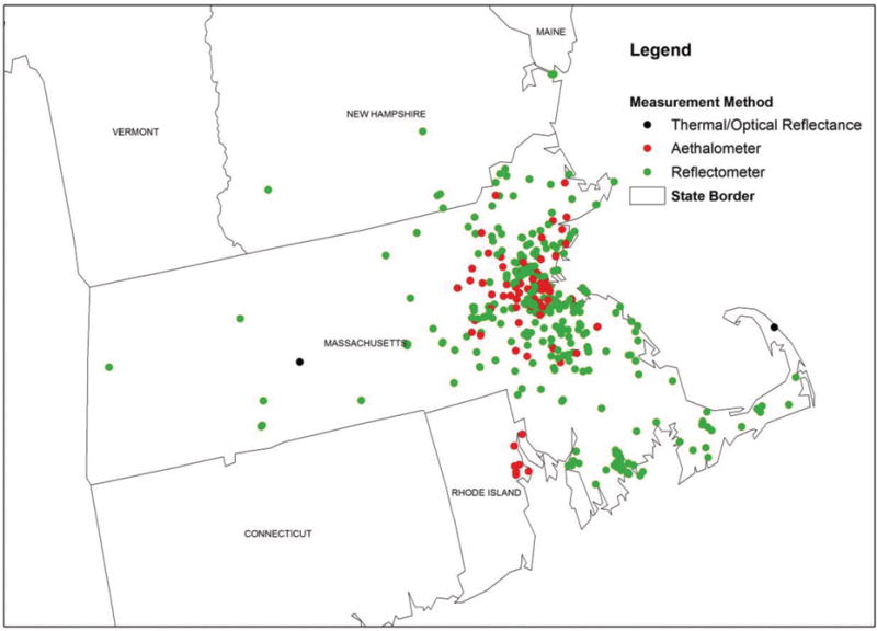
Locations of the 368 monitor sites

Sources of Measurements

As part of a National Institute of Environmental Health Sciences (NIEHS) funded study, we carried out measurements at 53 sites between 2006 and 2008 around the Boston area, which were selected based on gaps in previous spatial measurements. We obtained 2798 24-hour measurements using an Aethalometer® (Model AE-16 by Magee Scientific Corp.).

The Northeast States for Coordinated Air Use Management (NESCAUM) conducted a monitoring study to look at the spatial variability of pollution generated from traffic sources in the Boston area between 1999 and 2003 (Allen, 2014). BC was measured using an Aethalometer at 12 sites. This study provided 4767 24-h observations.

The Interagency Monitoring of Protected Visual Environments (“IMPROVE”) is a network of monitor sites in national parks and wilderness areas, that measures Elemental Carbon (EC) via thermal/optical reflectance. We obtained 2478 24-hour measurements from the Quabbin Summit and Cape Cod locations from 2001 to 2011.

The U.S. Environmental Protection Agency (EPA) requires states to monitor PM2.5. Teflon® filters used to collect 24-hour PM_2.5 ambient measurements throughout MA and Southern NH were obtained from the state environmental agencies, and we analyzed them for BC using a smokestain reflectometer (EEL Model M34D by Diffusion Systems Ltd). Reflectance was transformed to absorption coefficients according to ISO 9835. We obtained 6073 measurements from 23 sites in MA and 591 measurements from 7 sites in Southern NH for the years 2000 – 2011. We also obtained a total of 7285 Aethalometer BC observations from the RI Department of Environmental Management, from 7 sites between 2005 and 2011.

The Normative Aging study (NAS) is a longitudinal study of aging established by the Veterans Administration in 1961. We conducted indoor exposure monitoring between 2006 and 2010 at the homes of study participants. Measurements were taken in the main activity room of participants’ homes over the period of one week using a Teflon® filter and BC was also estimated using the smokestain reflectometer mentioned above. In order to approximate ambient BC from indoor measurements, we estimated the penetrance of outdoor pollutants by dividing weekly average ambient sulfate concentrations (which we measured at a site located on the roof of the Harvard T. H. Chan School of Public Health; HSPH) by indoor sulfate concentrations (estimated using X-ray fluorescence), and multiplied this by the indoor BC concentrations as follows:

$$B{C}_{\mathit{out}=B{C}_{in}\times \frac{S_{\mathit{out}}}{S_{in}}}$$

From this study we obtained 309 weeks of measurements at 262 addresses.

Spatial predictors

Proximity to transportation

We calculated distance to rail and identified the nearest type of rail service using the U.S. census topologically integrated geographic encoding and referencing system (TIGER) rail shapefiles. Type of road and traffic density data were obtained from the U.S. Department of Transportation Federal Highway Administration Highway Performance Monitoring System (HPMS). Distance to bus routes and length of bus routes within 50 and 100 m buffers was extracted using shapefiles from: Rhode Island Geographic Information System (RIGIS),(2014), the Southern New Hampshire Planning Commission (Kizak, 2014) and the Massachusetts Bay Transit Authority (“MassGIS Data - MBTA Bus Routes and Stops,” 2012). Distance to nearest truck route in meters was estimated using the Freight Analysis Framework (FAF) Network machine-readable data files. Finally, a visual inspection of satellite imagery from Google Earth was carried out to manually classify roads as surface, above surface-or subsurface. This was to control for overestimation of the impact of traffic when an address was close to a major road that is either underground or far above ground.

Topographical characteristics

We obtained elevation data from the national elevation data set (NED) (Maude, 2007) and calculated distance to coast using ArcGIS version 10.2.2 (ESRI, Redlands, CA).

Percentage surface water area within 2 and 10 km radii was also calculated in ArcGIS using surface water shapefiles from RIGIS (2014), the Shuttle Radar Topography Mission (SRTM) Water Body Data Files (Farr et al., 2007) and the Massachusetts Office of Geographic Information (MassGIS, 2012)

Neighborhood characteristics

We obtained percentages of land use according to three land use categories based on the United States Geological Survey (USGS) National Land Cover Dataset (NLCD) (Homer et al., 2004): low development, high development and impervious surfaces. Population density and percentage fuel use (oil, coal, electricity, wood, and solar) were available at the census block group level in the 2000 U.S. Census (US Census Bureau).

Temporal predictors

Temperature, wind speed, visibility, dew point, sea-level pressure, and relative humidity were obtained through the National Climatic Data Center (NCDC, n.d.). We retrieved data from the closest weather station to a given monitor that has non-missing data for these variables. Wind direction and daily height of the Planetary Boundary Layer (PBL) were obtained from the from the NOAA Reanalysis Data (Kalnay et al., 1996), available publicly at a spatial resolution of 32×32 km. The boundary layer strongly influences the dispersion of local pollutants and their concentration in the atmosphere (Angevine et al., 2013).

We also used average daily BC and PM_2.5 concentrations at the site located on the roof of the HSPH and operated by the HSPH Department of Environmental Health as temporal predictors. This has provided daily data since 1998. Furthermore, we included indicator variables for year, month, and weekday.

All temporal predictors with daily values were averaged over a week for NAS indoor measurements in order to match the week over which BC was measured.

Statistical methods

In order to make the measurements obtained using different methods comparable we carried out season specific calibrations using data from the abovementioned site located on the roof of the HSPH which provides concurrent EC, aethalometer and reflectance observations. EC and reflectance measurements were regressed separately against aethalometer data and an indicator variable for Year for both cold and warm seasons. We then adjusted the reflectance and EC measurements using regression-derived coefficients for each measurement method and each season. We then built our prediction model using nu-Support Vector Regression (nu-SVR) in R (version 3.0.1) with package e1071.

The support vector method was initially developed for classification problems and then extended to regression by Vapnik (Vapnik, 1995). The model is described in detail in Apprendix (A) and elsewhere (Smola & Schölkopf, 2004; Vapnik, 1995), but in brief the line of best fit is estimated in the following three steps:

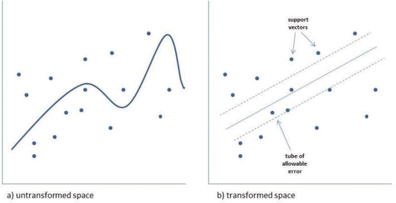
Mapping the data into a multidimensional feature space with the use of a kernel function. In the transformed space, linear relationships are estimated between the predictors and the variable of interest which appear as curves in the non-transformed covariate space, as shown in panel (a) of Figure 2. This transformation accounts for the non-linear relationships between predictors and the outcome, in this case BC levels.

We used a Gaussian radial basis function (RBF) kernel:

$$\mathrm{K}(\mathrm{x},\mathrm{x}\prime )=\exp (-\gamma {\left|\mathrm{x}-\mathrm{x}\prime \right|}^2),$$

where $\gamma =\frac{1}{2{\sigma }^2}$ and x and x′ are vectors of the predictors for each day for each location. Note that the expansion of the quadratic function within this Gaussian kernel contains nonlinear and product terms between all of the variables. Incorporating interactions was essential in allowing the effect of spatial variables to vary over time in our model.

Figure 2.

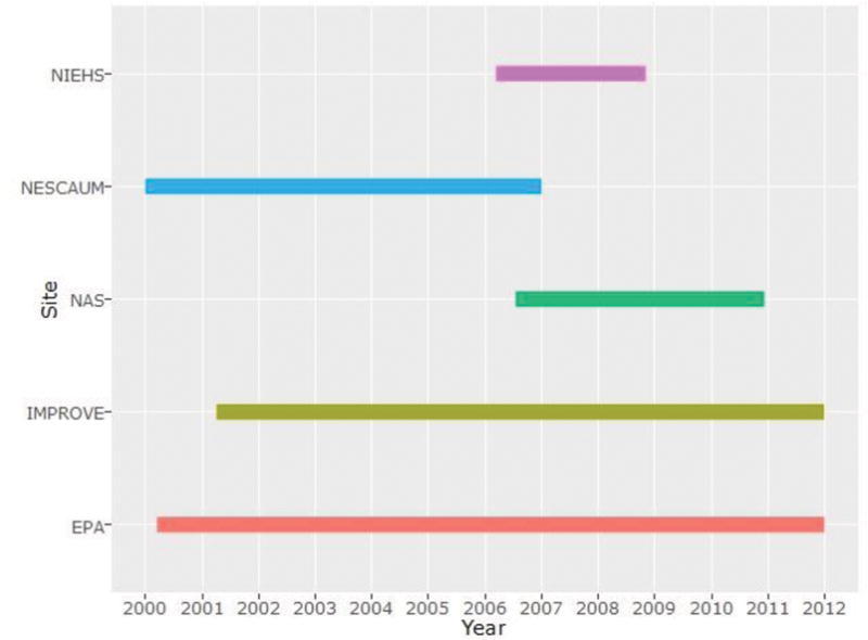
Duration of monitoring in each of the studies

Gamma controls the smoothness of the curves being fit to the data, and also determines how strongly those nonlinear relationships and interactions are penalized towards zero.

Specifying allowable error

In nu-SVR, a user defined variable named “nu” determines what percentage of observations can be estimated with error. Incorporating nu effectively treats small errors in prediction as ignorable and produces a model that has better performance in terms of reducing larger errors and therefore avoiding overfitting. This can be thought of as placing a “tube” around the regression line where any observations lying within the tube are ignored (see Figure 2 panel b). The prediction error of observations outside the tube is then minimized – these observations are known as support vectors.

Incorporation of a ridge penalty

Incorporation of a ridge penalty which minimizes the prediction error but simultaneously puts a penalty on the coefficients. This results in coefficient shrinkage which also prevents overfitting. Therefore a large number of correlated predictors can be input into a nu-SVR and the model will use data only from those that improve performance.

We used the Gaussian kernel and selected gamma by running 10 fold cross validation using multiple values and then selecting the value which gave the highest cross validated R². Nu was also selected by running 10 fold CV using multiple values and selecting one that produced the highest cross validated R².

To account for the seasonal variability in meteorological variables and BC emission patterns, the model was run separately in cold (November to April) and warm (May to October) seasons. Longitude and latitude were also added, so that the model could incorporate spatial variability, in particular differences in predictive ability of a given land use or meteorological covariate across space.

We then carried out simply gradient boosting by taking the residuals from the nu-SVR model and testing whether or not they were still associated with any of our explanatory variables using a GAM. Significant variables and smooth terms were incorporated and the predicted residuals from this model were then added to our nu-SVR predictions.

Finally, in order to evaluate model fit, first we calculated the R² between predicted and observed concentrations. We then applied 10-fold cross validation (10-fold CV) which comprises: splitting the data into 10 equal parts, removing one tenth of the data and using the remaining observations to train the model and then testing the model on the excluded observations. This was repeated 10 times, each time excluding one tenth of the data and the Pearson R2 between observed and predicted values was averaged over the ten testing sets. We chose 10 fold cross validation rather than leave one out validation as it allows us to exclude multiple locations and multiple days and is thus a fairer test. It also shows us if our model has been overfit if it performs poorly in the left-out data.

We also carried out sensitivity analyses in order to see the effect of removing any single study from the data by excluding one study at a time, training the model and then testing it on data from the left-out study. In addition, we evaluated how well the model captures temporal variance by taking the difference between the daily concentrations and the annual means of both predicted and observed values at each monitor and then regressing the former against the latter. We were able to do this for all years except for 2000 which had only 310 observations. We also evaluated how well the model captures long-term exposures by separating out the spatial component of BC at each monitoring location using a regression model to remove the temporal variation and isolate that spatial component. Specifically, we regressed daily monitored values against indicator variables for each day of the week in each week of the year in each year, and indicator variables for each monitor. The coefficient for each monitor captures the average spatial contrast between monitors, since temporal variations have been removed.

Then, we took our prediction model, and predicted black carbon concentrations at each monitor, for the years each monitor operated. We averaged those predictions over the year or years. This captures the long term spatial pattern of the predictions from our model. Finally, we regressed the spatial contrast in monitor values (from the first regression) against the mean predictions from our model.

Results

Our calibration adjusted values had a mean of 0.63 μg/m³, a maximum of 4.46 μg/m³ and a standard deviation of 0.42 μg/m³

For our model, the agreement between observed and nu-SVR predicted ambient BC was good in both cold (10-fold CV R² = 0.73) and warm seasons (CV R² = 0.75). After adding predicted residuals to nu-SVR predictions, the 10-fold CV R² increased to 0.87 for cold and 0.79 for warm.

Figure 4 shows plots of predicted and observed values. The slope of the relationship between observed and nu-SVR predicted values was 1.1. in the cold season and 1.08 in the warm season. The slope of the relationship between observed and residual-adjusted predictions was 1.07 in the cold season and 1.02 in the warm season.

Figure 4.

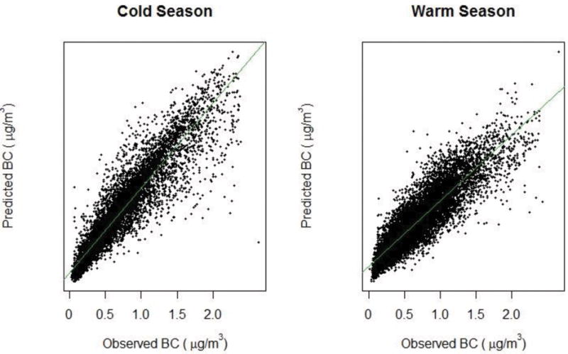
Relationships between the observed-predicted BC concentrations in cold and warm periods.

Figure 3 shows the spatial pattern of predicted BC on four days in 2007: one day from each season, namely; February 18^th, April 18^th, July 21^st and October 18^th on a 200 m grid. The maps depicting February 18^th and July 21^st, which were a Sunday and Saturday respectively, show reduced spatial variability and much lower BC concentrations compared to the other two dates, which were weekdays. Furthermore, concentrations are much higher on October 18^th compared to April 18^th which are both weekdays, as the low planetary boundary layer (PBL) on this day in October reduces the dilution of air pollutants. In contrast, the higher PBL value combined with higher wind speed on the date chosen for April increases pollutant dispersion and leads to lower predictions (Table 1.) In addition, concentrations are higher near major roads, particularly those with heavy bus traffic.

Figure 3.

Graphic representation of nu-Support Vector regression

Table 1.

Weather conditions on days with mapped concentrations

Date	Temperature (F)	Wind Speed (knots)	Visibility (miles)	Relative Humidity (%)	Dewpoint (F)	Sea Level Pressure (mbar)	Height of the Planetary Boundary Layer (m)
02/18/07	26	6	9	57	13	1004	777
04/18/07	40	11	6	87	37	1006	1153
07/21/07	68	7	10	61	54	1014	924
10/18/07	60	3	5	85	55	1015	455

Figure 4 shows the trend in annual BC concentrations at different proximities to both truck routes and bus routes, at addresses of NAS participants. It appears that BC concentrations have declined more at addresses near truck routes compared to addresses that are further away, indicating spatial variability in rates of decline. For example, as emissions standards have become stricter, the effect of distance to truck route on observed concentrations has diminished over time.

On the other hand, exposures at locations within 140m of a Regional Transit Authority bus route seem only slightly higher than exposures that are 7630 m away of more and this difference shrinks in 2004 and 2007. As expected, concentrations near bus routes declined around 2002 when the MBTA bus fleet underwent several changes including the switch to low sulfur diesel fuel and installation of particulate matter filters in older vehicles (MBTA Scorecard, 2009). The second declining trend occurs after 2005 when major road structure changes were completed in Boston. PM emissions from buses also declined steeply during this time (MBTA Scorecard, 2009).

Sensitivity Analysis

The R2 in the left out studies are shown in Table 2. We can see that predictions remained relatively good (R2 of approximately 0.8) regardless of which study was left out indicating that our results are not driven by data from one study even though the collection methods were different.

Table 2.

R² and Slope between predicted and observed values for each held out study

	EPA	IMPROV	NSCA	PPG2	RI	NAS
R2	0.81	0.88	0.81	0.81	0.78	0.84
Slope	1.24	1.15	1.25	1.24	1.26	1.19

The results of the temporal cross validation also showed a good fit with R² values ranging from 0.70 to 0.86 (see Table 3). The spatial cross validation yielded an R² of 0.91 which indicates that our model captures long-term exposures quite well.

Table 3.

R² between predicted and observed differences from the mean by year

Year	R2
2001	0.70
2002	0.73
2003	0.71
2004	0.75
2005	0.77
2006	0.74
2007	0.77
2008	0.73
2009	0.79
2010	0.82
2011	0.86

Discussion

We have generated daily estimates of ambient BC in MA, RI and Southern NH from 2000 to 2011. This model builds on our previous BC model (Gryparis et al 2007), not only by expanding the geographic region but also by introducing several improvements. First, we added more monitors with repeated measurements to better capture temporal variability at different locations. Second, we also used machine learning, specifically a nu-SVR regression in order to better incorporate interactions and nonlinearities in the relationships between predictors and BC, and to address the erratic predictions at model boundaries of the previous model. The use of nu-SVR also enabled us to include interactions between all spatial and temporal terms without overfitting, as regularization shrinks the coefficients of terms that are not important. Interactions also allow for the effect of spatial variables to vary over time, since SVR allows these spatial variables to interact with indicator variables for year, month and weekday, which reflects real world changes. The further use of a GAM to predict the residuals improves the fit of the model and complements the nu-SVR approach.

When comparing the performance of this model applied in New England with other land use regression models applied elsewhere using detailed spatial monitoring data (Brauer et al., 2003; Eeftens et al., 2012; Urman et al., 2014), it is important to emphasize that the time frames considered in the various studies vary widely and make direct comparisons difficult. For instance, while existing studies reported cross validated R² values from 36 up to 95%, data was only collected over a period of 3 years in the ESCAPE (European Study of Cohorts for Air Pollution Effects) study (Eeftens et al., 2012), 13 months in the California study (Urman et al., 2014) and up to 16 months in the Brauer study. Therefore, when these models are used to extrapolate exposures to future years, they will likely overestimate exposure (as ambient concentrations have been declining steadily), and past exposures will likely be underestimated for the same reason. This introduces exposure error into epidemiologic studies using such models.

Our use of monitoring data for over a decade, and allowing for interaction between all land use predictors and year of study, captures spatio-temporal variability in exposure that was not captured effectively by previous models. In addition, most previous models can only predict long-term exposures (i.e. annual or 8 week average), while our model can predict daily concentrations which will allow studies that use these data to look at the effects of both short and long-term exposures.

Other models (Crouse et al., 2016; Li, Henze, Jack, Henderson, & Kinney, 2016) which included data over a long period of time, did not use directly measured BC. Rather, the outputs from GEOS-chem chemical transport model and remote sensing data on aerosol optical depth were used to generate estimates over a large area (resolution of 10×10 km).

While our model has the advantages discussed above, it also has some limitations. Although we did add observations in Cape Cod by using residential monitors from NAS indoor data and data from the IMPROVE site, there was a lack of monitors with a large number of repeated measures. We also do not have many available monitors in Western MA. Therefore there exist a few areas with sparse monitor coverage. This may be partly offset by our inclusion of longitude and latitude in the model, which enabled us to capture patterns of emissions rendering spatially homogenous areas distinct. Another limitation is that BC was measured by several methods; we attempted to account for this by calibrating reflectometer and thermal/optical measurements to aethalometer readings.

In summary, we have successfully built a model that can be used to accurately estimate short and long-term exposures to BC and will be useful for studies looking at various health outcomes in MA, RI and Southern NH.

Figure 5.

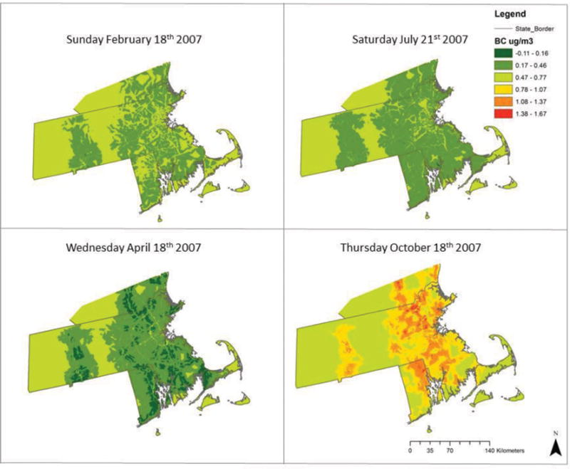
Maps of predicted Black Carbon concentrations in μg/m³ on four different days in 2007.

Figure 6.

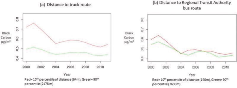
Changes in mean annual Black Carbon concentrations in μg/m³ at selected residential locations

Highlights.

• Ambient Black Carbon has many health effects, good exposure assessment is needed

• We used data from 368 monitors from Massachusetts, Rhode Island and New Hampshire

• Predictors included 24,301 measurements over 12 years plus spatial and temporal terms.

• Nu-Support Vector Regression and a generalized additive model were applied for prediction

• 10 fold cross validated R² was good in cold (0.87) and warm seasons (0.79)

References

- Alexeeff SE, Coull BA, Gryparis A, Suh H, Sparrow D, Vokonas PS, Schwartz J. Medium-Term Exposure to Traffic-Related Air Pollution and Markers of Inflammation and Endothelial Function. Environmental Health Perspectives. 2011;119(4):481–486. doi: 10.1289/ehp.1002560. https://doi.org/10.1289/ehp.1002560. [DOI] [PMC free article] [PubMed] [Google Scholar]
- Allen G. Analysis of Spatial and Temporal Trends of Black Carbon in Boston. Northeast States for Coordinated Air Use Management 2014 [Google Scholar]
- Analitis A, Katsouyanni K, Dimakopoulou K, Samoli E, Nikoloulopoulos AK, Petasakis Y, Pekkanen J. Short-Term Effects of Ambient Particles on Cardiovascular and Respiratory Mortality. Epidemiology. 2006;17(2):230–233. doi: 10.1097/01.ede.0000199439.57655.6b. https://doi.org/10.1097/01.ede.0000199439.57655.6b. [DOI] [PubMed] [Google Scholar]
- Angevine WM, Brioude J, McKeen S, Holloway JS, Lerner BM, Goldstein AH, Bon D. Pollutant transport among California regions: CALIFORNIA POLLUTANT TRANSPORT. Journal of Geophysical Research: Atmospheres. 2013;118(12):6750–6763. https://doi.org/10.1002/jgrd.50490. [Google Scholar]
- Beelen R, Hoek G, van den Brandt PA, Goldbohm RA, Fischer P, Schouten LJ, Brunekreef B. Long-Term Effects of Traffic-Related Air Pollution on Mortality in a Dutch Cohort (NLCS-AIR Study) Environmental Health Perspectives. 2008;116(2):196–202. doi: 10.1289/ehp.10767. https://doi.org/10.1289/ehp.10767. [DOI] [PMC free article] [PubMed] [Google Scholar]
- Brauer M, Hoek G, van Vliet P, Meliefste K, Fischer P, Gehring U, Brunekreef B. Estimating Long-Term Average Particulate Air Pollution Concentrations: Application of Traffic Indicators and Geographic Information Systems. Epidemiology. 2003;14(2):228–239. doi: 10.1097/01.EDE.0000041910.49046.9B. https://doi.org/10.1097/01.EDE.0000041910.49046.9B. [DOI] [PubMed] [Google Scholar]
- Bremner SA, Anderson HR, Atkinson RW, McMichael AJ, Strachan DP, Bland JM, Bower JS. Short-term associations between outdoor air pollution and mortality in London 1992–4. Occupational and Environmental Medicine. 1999;56(4):237–244. doi: 10.1136/oem.56.4.237. https://doi.org/10.1136/oem.56.4.237. [DOI] [PMC free article] [PubMed] [Google Scholar]
- Clougherty JE, Wright RJ, Baxter LK, Levy JI. Land use regression modeling of intraurban residential variability in multiple traffic-related air pollutants. Environ Health. 2008;7(1):17. doi: 10.1186/1476-069X-7-17. [DOI] [PMC free article] [PubMed] [Google Scholar]
- Crouse DL, Philip S, van Donkelaar A, Martin RV, Jessiman B, Peters PA, Burnett RT. A New Method to Jointly Estimate the Mortality Risk of Long-Term Exposure to Fine Particulate Matter and its Components. Scientific Reports. 2016;6:18916. doi: 10.1038/srep18916. https://doi.org/10.1038/srep18916. [DOI] [PMC free article] [PubMed] [Google Scholar]
- Dockery DW, Pope CA, Xu X, Spengler JD, Ware JH, Fay ME, Speizer FE. An Association between Air Pollution and Mortality in Six U.S. Cities. New England Journal of Medicine. 1993;329(24):1753–1759. doi: 10.1056/NEJM199312093292401. https://doi.org/10.1056/NEJM199312093292401. [DOI] [PubMed] [Google Scholar]
- Eeftens M, Beelen R, de Hoogh K, Bellander T, Cesaroni G, Cirach M, Hoek G. Development of Land Use Regression Models for PM2.5, PM2.5 Absorbance, PM10 and PMcoarse in 20 European Study Areas; Results of the ESCAPE Project. Environmental Science & Technology. 2012;46(20):11195–11205. doi: 10.1021/es301948k. https://doi.org/10.1021/es301948k. [DOI] [PubMed] [Google Scholar]
- Farr TG, Rosen PA, Caro E, Crippen R, Duren R, Hensley S, Alsdorf D. The Shuttle Radar Topography Mission. Reviews of Geophysics. 2007;45(2) https://doi.org/10.1029/2005RG000183. [Google Scholar]
- Filleul L, Rondeau V, Vandentorren S, Moual NL, Cantagrel A, Annesi-Maesano I, Baldi I. Twenty five year mortality and air pollution: results from the French PAARC survey. Occupational and Environmental Medicine. 2005;62(7):453–460. doi: 10.1136/oem.2004.014746. https://doi.org/10.1136/oem.2004.014746. [DOI] [PMC free article] [PubMed] [Google Scholar]
- Gryparis A, Coull BA, Schwartz J, Suh HH. Semiparametric latent variable regression models for spatiotemporal modelling of mobile source particles in the greater Boston area. Journal of the Royal Statistical Society: Series C (Applied Statistics) 2007;56(2):183–209. [Google Scholar]
- Hajek P. Predicting Common Air Quality Index – The Case of Czech Microregions. Aerosol and Air Quality Research. 2015 https://doi.org/10.4209/aaqr.2014.08.0154.
- Hoek G, Beelen R, de Hoogh K, Vienneau D, Gulliver J, Fischer P, Briggs D. A review of land-use regression models to assess spatial variation of outdoor air pollution. Atmospheric Environment. 2008;42(33):7561–7578. https://doi.org/10.1016/j.atmosenv.2008.05.057. [Google Scholar]
- IMPROVE. (n.d.) Retrieved February 19, 2016, from http://vista.cira.colostate.edu/improve/
- Jansen KL, Larson TV, Koenig JQ, Mar TF, Fields C, Stewart J, Lippmann M. Associations between Health Effects and Particulate Matter and Black Carbon in Subjects with Respiratory Disease. Environmental Health Perspectives. 2005;113(12):1741–1746. doi: 10.1289/ehp.8153. [DOI] [PMC free article] [PubMed] [Google Scholar]
- Kalnay E, Kanamitsu M, Kistler R, Collins W, Deaven D, Gandin L, Joseph D. The NCEP/NCAR 40-Year Reanalysis Project. Bulletin of the American Meteorological Society. 1996;77(3):437–471. https://doi.org/10.1175/1520-0477(1996077<0437:TNYRP>2.0.CO;2) [Google Scholar]
- Kizak A. New Hampshire Bus Shapefiles (n.d.) [Google Scholar]
- Krewski D, Jerrett M, Burnett RT, Ma R, Hughes E, Shi Y, et al. Extended follow-up and spatial analysis of the American Cancer Society study linking particulate air pollution and mortality. Health Effects Institute; Boston, MA: 2009. Retrieved from http://scientificintegrityinstitute.net/Krewski052108.pdf. [PubMed] [Google Scholar]
- Künzli N, Jerrett M, Mack WJ, Beckerman B, Labree L, Gillil F, Hodis HN. Ambient air pollution and atherosclerosis in Los Angeles. Environ Health Perspect. 2005;113:201–206. doi: 10.1289/ehp.7523. [DOI] [PMC free article] [PubMed] [Google Scholar]
- Laden F, Neas LM, Dockery DW, Schwartz J. Association of fine particulate matter from different sources with daily mortality in six US cities. Environ Health Perspect. 2000;108:941–947. doi: 10.1289/ehp.00108941. (n.d.) [DOI] [PMC free article] [PubMed] [Google Scholar]
- Lepeule J, Laden F, Dockery D, Schwartz J. Chronic Exposure to Fine Particles and Mortality: An Extended Follow-up of the Harvard Six Cities Study from 1974 to 2009. Environmental Health Perspectives. 2012;120(7):965–970. doi: 10.1289/ehp.1104660. https://doi.org/10.1289/ehp.1104660. [DOI] [PMC free article] [PubMed] [Google Scholar]
- Lepeule J, Litonjua AA, Coull B, Koutrakis P, Sparrow D, Vokonas PS, Schwartz J. Long-Term Effects of Traffic Particles on Lung Function Decline in the Elderly. American Journal of Respiratory and Critical Care Medicine. 2014;190(5):542–548. doi: 10.1164/rccm.201402-0350OC. https://doi.org/10.1164/rccm.201402-0350OC. [DOI] [PMC free article] [PubMed] [Google Scholar]
- Li Y, Henze DK, Jack D, Henderson BH, Kinney PL. Assessing public health burden associated with exposure to ambient black carbon in the United States. Science of The Total Environment. 2016;539:515–525. doi: 10.1016/j.scitotenv.2015.08.129. https://doi.org/10.1016/j.scitotenv.2015.08.129. [DOI] [PMC free article] [PubMed] [Google Scholar]
- Lu WZ, Wang WJ. Potential assessment of the “support vector machine” method in forecasting ambient air pollutant trends. Chemosphere. 2005;59(5):693–701. doi: 10.1016/j.chemosphere.2004.10.032. https://doi.org/10.1016/j.chemosphere.2004.10.032. [DOI] [PubMed] [Google Scholar]
- MassGIS Data – MBTA Bus Routes and Stops. 2012 Apr 4; Retrieved January 7, 2016, from http://www.mass.gov/anf/research-and-tech/it-serv-and-support/application-serv/office-of-geographic-information-massgis/datalayers/mbtabus.html.
- Maynard D, Coull BA, Gryparis A, Schwartz J. Mortality risk associated with short-term exposure to traffic particles and sulfates. Environmental Health Perspectives. 2007;115(5):751–755. doi: 10.1289/ehp.9537. https://doi.org/10.1289/ehp.9537. [DOI] [PMC free article] [PubMed] [Google Scholar]
- MBTA Scorecard. 2009 Retrieved from https://www.mbta.com/uploadedfiles/About_the_T/Score_Card/ScoreCard-2009-11.pdf.
- Natekin A, Knoll A. Gradient boosting machines, a tutorial. Frontiers in Neurorobotics. 2013;7 doi: 10.3389/fnbot.2013.00021. https://doi.org/10.3389/fnbot.2013.00021. [DOI] [PMC free article] [PubMed] [Google Scholar]
- NCDC. The national climatic data center data inventories 2010 (n.d.) [Google Scholar]
- Office of Geographic Information (MassGIS), Commonwealth of Massachusetts, MassIT. MassGIS Data – MassDEP Hydrography (1:25,000) 2012 Apr 2; Retrieved August 3, 2017,, from http://www.mass.gov/anf/research-and-tech/it-serv-and-support/application-serv/office-of-geographic-information-massgis/datalayers/hd.html.
- Ostro B, Feng WY, Broadwin R, Green S, Lipsett M. The Effects of Components of Fine Particulate Air Pollution on Mortality in California: Results from CALFINE. Environmental Health Perspectives. 2007;115(1):13–19. doi: 10.1289/ehp.9281. [DOI] [PMC free article] [PubMed] [Google Scholar]
- Pope CA, Thun MJ, Namboodiri MM, Dockery DW, Evans JS, Speizer FE, Heath CW. Particulate Air Pollution as a Predictor of Mortality in a Prospective Study of U.S. Adults. American Journal of Respiratory and Critical Care Medicine. 1995;151(3_pt_1):669–674. doi: 10.1164/ajrccm/151.3_Pt_1.669. https://doi.org/10.1164/ajrccm/151.3_Pt_1.669. [DOI] [PubMed] [Google Scholar]
- Power MC, Weisskopf MG, Alexeeff SE, Coull BA, Spiro A, Schwartz J. Traffic-Related Air Pollution and Cognitive Function in a Cohort of Older Men. Environmental Health Perspectives. 2010;119(5):682–687. doi: 10.1289/ehp.1002767. https://doi.org/10.1289/ehp.1002767. [DOI] [PMC free article] [PubMed] [Google Scholar]
- Rhode Island Geographic Information System (RIGIS) 2014 Retrieved January 7, 2016, from http://www.rigis.org.
- Ryan PH, LeMasters GK. A review of land-use regression models for characterizing intraurban air pollution exposure. Inhalation Toxicology. 2007;19(Suppl 1):127–133. doi: 10.1080/08958370701495998. https://doi.org/10.1080/08958370701495998. [DOI] [PMC free article] [PubMed] [Google Scholar]
- Sasser E. Report to Congress on Black Carbon. United States Environmental Protection Agency; 2012. (No. EPA-450/R-12001) [Google Scholar]
- Schwartz J, Alexeeff SE, Mordukhovich I, Gryparis A, Vokonas P, Suh H, Coull BA. Association between long-term exposure to traffic particles and blood pressure in the Veterans Administration Normative Aging Study. Occupational and Environmental Medicine. 2012;69(6):422–427. doi: 10.1136/oemed-2011-100268. https://doi.org/10.1136/oemed-2011-100268. [DOI] [PMC free article] [PubMed] [Google Scholar]
- Schwartz Joel, Marcus A. Mortality and Air Pollution J London: A Time Series Analysis. American Journal of Epidemiology. 1990;131(1):185–194. doi: 10.1093/oxfordjournals.aje.a115473. [DOI] [PubMed] [Google Scholar]
- Smith KR, Jerrett M, Anderson HR, Burnett RT, Stone V, Derwent R, Thurston G. Public health benefits of strategies to reduce greenhouse-gas emissions: health implications of short-lived greenhouse pollutants. The Lancet. 2009;374(9707):2091–2103. doi: 10.1016/S0140-6736(09)61716-5. https://doi.org/10.1016/S0140-6736(09)61716-5. [DOI] [PMC free article] [PubMed] [Google Scholar]
- Smola AJ, Schölkopf B. A tutorial on support vector regression. Statistics and Computing. 2004;14(3):199–222. https://doi.org/10.1023/B:STCO.0000035301.49549.88. [Google Scholar]
- Sotomayor-Olmedo A, Aceves-Fernández MA, Gorrostieta-Hurtado E, Pedraza-Ortega C, Ramos-Arreguín JM, Vargas-Soto JE. Forecast Urban Air Pollution in Mexico City by Using Support Vector Machines: A Kernel Performance Approach. International Journal of Intelligence Science. 2013;03(03):126–135. https://doi.org/10.4236/ijis.2013.33014. [Google Scholar]
- Suglia SF, Gryparis A, Wright RO, Schwartz J, Wright RJ. Association of Black Carbon with Cognition among Children in a Prospective Birth Cohort Study. American Journal of Epidemiology. 2008;167(3):280–286. doi: 10.1093/aje/kwm308. https://doi.org/10.1093/aje/kwm308. [DOI] [PubMed] [Google Scholar]
- Urman R, Gauderman J, Fruin S, Lurmann F, Liu F, Hosseini R, McConnell R. Determinants of the spatial distributions of elemental carbon and particulate matter in eight Southern Californian communities. Atmospheric Environment. 2014;86:84–92. doi: 10.1016/j.atmosenv.2013.11.077. https://doi.org/10.1016/j.atmosenv.2013.11.077. [DOI] [PMC free article] [PubMed] [Google Scholar]
- US Census Bureau. Geography: TIGER Products. (n.d.) Retrieved March 11, 2016, http://www.census.gov/geo/maps-data/data/tiger.html.
- Vapnik VN. The Nature of Statistical Learning Theory. New York, NY: Springer New York; 1995. Retrieved from http://link.springer.com/10.1007/978-1-4757-2440-0. [Google Scholar]
- Wilker EH, Mittleman MA, Coull BA, Gryparis A, Bots ML, Schwartz J, Sparrow D. Long-term Exposure to Black Carbon and Carotid Intima-Media Thickness: The Normative Aging Study. Environmental Health Perspectives. 2013 doi: 10.1289/ehp.1104845. https://doi.org/10.1289/ehp.1104845. [DOI] [PMC free article] [PubMed]