

Abstract
In this article, we review physics-based models of collective cell motility. We discuss a range of techniques at different scales, ranging from models that represent cells as simple self-propelled particles to phase field models that can represent a cell’s shape and dynamics in great detail. We also extensively review the ways in which cells within a tissue choose their direction, the statistics of cell motion, and some simple examples of how cell-cell signaling can interact with collective cell motility. This review also covers in more detail selected recent works on collective cell motion of small numbers of cells on micropatterns, in wound healing, and the chemotaxis of clusters of cells.
1. Introduction
Many isolated eukaryotic cells are able to move in a crawling fashion. This movement, which can be either spontaneous or guided by an external cue, involves a number of critical steps. First, the cell body needs to be extended in the direction of movement through the polymerization of actin. Second, parts of the cell body away from the extensions need to be retracted, facilitated by the motor protein myosin. Finally, there needs to be enough friction between the cell and its environment to be able to generate net movement. How the cell integrates these steps, how external cues are interpreted, and how noise may play a role in cell motility are all active fields of experimental and theoretical research [1, 2, 3, 4, 5, 6].
Recently, the focus of motility research has broadened to include collective cell migration. Examples of collective motility in biology are plentiful. One example, which has enjoyed significant interest, is wound healing [7]. Here, cells move towards the wound in order to remove harmful bacteria and to close the tissue [8]. Another example comes from developmental biology where groups of cells migrate to distinct locations within the embryo to carry out specific tasks [9, 10]. Not all examples are beneficial to the organism, however. During cancer metastasis, groups of cancer cells migrate through tissue, resulting in the spreading of tumors [11]; a broad range of recent studies suggest that metastasis by clusters of cancer cells may be more dangerous than single-cell metastasis [12]. Clearly, understanding how these groups migrate and coordinate their movement can be beneficial in the development of therapies.
In most examples, collective motility is not simply the result of many individually moving cells. Instead, cells crawl together in a coordinated way, resulting in behavior that is not seen in individual cells. For example, expanding cell monolayers often exhibit the spontaneous formation of finger-like instabilities with specialized cells at their tips [13, 14]. Also, several cell types exhibit emergent chemotaxis in the absence of individual cell chemotaxis [15, 16, 17]; groups of cells can also be governed by a few leader cells [18]. How these collective behaviors arise is an continuing and active area of research [19, 20].
Where does physics, and more specifically, physical modeling enter the process of collective cell motion? As already mentioned, cell motion requires protrusions, retractions, and friction and thus rely on a balance of forces. Therefore, describing the motion of cells in a quantitative manner requires solving equations that incorporate these forces [21, 22]. In addition, some of these forces are generated through the action of signaling molecules which are part of signaling networks [23]. Typical eukaryotic cell sizes are in the range of 10–100 μm. As a consequence, moving cells exhibit a distinct spatial asymmetry with some signaling components localized in the front and others localized in the back of the cell. Modeling this asymmetry, often called cell polarity, requires solving sets of coupled reaction diffusion equations [6, 24]. Likewise, modeling the interactions between different cells can involve cell-cell communication in the form of diffusive components and thus spatially extended systems. In addition, noise in these signaling networks might play a significant role and addressing its role requires tools from statistical physics [25, 26]. Finally, the morphology of the cell changes as it is moving and an accurate representation of a moving, deforming boundary can be formulated using techniques developed in physics [27, 28, 29].
This review focuses on modeling of collective cell motility and for a detailed overview of experimental results in collective motility we refer to recent reviews, for example by Friedl and Gilmour [11] or Mayor and Etienne-Manneville [30]. Furthermore, we also restrict our review to eukaryotic biological systems and do not discuss bacterial systems nor do we review synthetic active matter, which also displays collective motion. Readers primarily interested in synthetic or bacterial collective motion should consult reviews by Ramaswamy [31] and Marchetti et al. [32]. Our focus is also on models that resolve individual cells; continuum models are discussed by Marchetti et al. [32]; agent-based models without resolving individual cells are reviewed by Van Liedekerke et al. [33]. We will also primarily discuss collective cell migration on substrates, where the links between two-dimensional models and in vitro experiments are simpler.
We believe collective cell migration is an area where modelers can contribute a great deal to new understanding in cell biology. Experimental interventions to alter molecular mechanisms in cell motility often influence several features at once, leading to ambiguity in analyzing results. Models allow us to have accurate and quantitative control over any proposed mechanism, which is only rarely possible experimentally. Models can not only determine whether a mechanism would be feasible, they can typically also generate predictions that can be tested in experiments. In addition, in moving from verbal to mathematical models, we often find that we must include additional assumptions, which can change our results. For instance, we found that modeling contact inhibition of locomotion in [34] yielded strongly different results depending on whether this effect was isotropic around the cell, or localized to its front. Testing these assumptions is also a source for new interesting experimental ideas.
Due to space limitations we are not able to cite all relevant studies and we apologize to our colleagues for these omissions. Our review is organized as follows: we will first describe the basic ingredients of collective motility, will discuss what a collective cell model should incorporate, and will give an overview of the various modeling techniques that have been applied to the problem (Section 2). In Section 3 we will present several examples where modeling has resulted in a better understanding of the biology of collective motility and we will conclude with some possible future directions in Section 4.
2. What is a collective cell motility model? Basic elements and models applied
Tissues are composed of interacting collections of cells – an ensemble of flowing, actively crawling objects. Is a collective cell motility model then just merely an extension of the physics of soft active materials [32]? We argue that this is not the case. Cells cannot necessarily be thought of as generic active particles: they may be highly heterogeneous, with different internal states, they can engage in long-range chemical communication, and actively respond to mechanical forces exerted on them. Furthermore, cells are able to alter their properties as a response of their environment, for example by changing their gene expression.
Our main focus are recent advancements in the modeling of collective cell migration, and applications to wound healing, development, and in vitro model systems. In this section, we will discuss more broadly what we view as the critical elements of any model of collective cell migration. We argue there are four key elements that should be explicitly specified in any collective cell motility model that spans from the single-cell to the collective level: 1) the motility of single cells within the collective, including characteristic speed and orientation distributions, 2) the representation of cell shape and consequent mechanical interactions (e.g. cell-cell adhesion), 3) the polarity mechanism: how does a cell choose its direction?, and 4) potential biochemical signaling between cells. While in many models, these elements are linked – e.g. the cell’s direction may arise from its shape – we believe these points should be highlighted in any model. We address these elements, and give examples of how they are handled in different simulations, in the following subsections (Section 2.1–2.4). Our discussion here is not meant to be exhaustive; Van Liedekerke et al. present a more complete review of agent-based models of cell motility, including some models that do not resolve individual cells [33]. We also will not discuss cell division in detail, as many of the experiments we discuss involve either a fixed number of cells, or can be modeled in the absence of division.
2.1. Cell speed and orientation
Single cell motility and cell shape have been extensively characterized with both experiment and modeling. As an initial step in any cell-level model of collective cell migration, it is important to characterize how single cells would move in the absence of neighbors. This is, of course, a complex question in its own right, and provides a great deal of degrees of freedom in modeling collective cell migration. Here, we wish to highlight some of the choices that have to be made implicitly or explicitly by modelers in developing statistical models of a cell’s speed, orientation, and shape.
First, we will consider the statistics of a cell’s velocity. The key aspects are: 1) the distribution of the cell’s velocity, and 2) the cell’s persistence – the time scale over which its velocity changes. In Fig. 1 we illustrate three common distributions of cell velocities in two dimensions: a simple Gaussian, in which the velocities are peaked at zero, polarized, in which the most common velocities have nonzero magnitude, and intermittent, in which cells switch between states with low and high typical speeds. All three of these types can be observed in single-cell trajectories [35]. The distribution of velocities is a useful tool to characterize any single-cell model. However, for concreteness, in Fig. 1, we show trajectories simulated for a simple self-propelled particle model, where an overdamped cell is driven by a fluctuating active force. The Newtonian equation of motion for a cell in the overdamped, low Reynolds number environment of the cell is Factive − γvcell = 0, where −γv is the frictional force between the cell and the substrate. The active force is in the direction of the cell’s polarity p, which obeys a stochastic differential equation. Together, this model is:
| (1) |
| (2) |
where ξ(t) is a Gaussian Langevin force with 〈ξi(t)ξj(t′)〉 = δijδ(t−t′) with δij the Kronecker delta and the indices i, j run over the spatial dimensions of the model. We have chosen in Eqs. 1–2 to use units where v is exactly equal to the cell’s polarity p. Depending on the polarity potential W (p) and the memory kernel K(t), this model can produce a wide variety of different types of cell behavior – and this single-cell behavior can alter the dynamics of collective cell migration. There is a great deal of literature on models of this sort: we note in particular [36], who derive models related to Eq. 2 directly from cell data, and [37], who review the broad literature on active Brownian particles as modeled by equations resembling Eq. 2. Both of these references address many subtleties that we will gloss over. We will build on the model of Eqs. 1–2 later in this review, introducing multi-cell models that extend it.
Figure 1. Examples of characteristic velocity distributions.
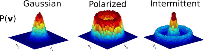
These basic phenotypes can be realized in many types of models. We have illustrated them in a simple Langevin model, v = p, with , where and ξ(t) is a Gaussian Langevin force with 〈ξi(t)ξj(t′)〉 = δijδ(t−t′) with δij the Kronecker delta. This corresponds to Eq. 1–Eq. 2 with K(t) = 0 – i.e. no long-term memory. We use (a1, a2, a3) = (2,0,0), (−2,3,0), and (3.2, −4,1) for the Gaussian, polarized, and intermittent examples, respectively.
The model of Eq. 1–2 treats the velocity and polarity of the cell as exactly equal, and we could have phrased it just as easily solely in terms of the velocity – as is done in [36]. However, distinguishing between velocity and polarity will be useful in models that have many cells. In those models, it makes sense to view the velocity of the cell as a snapshot of the present motion, but think of the polarity of the cell as indicating how the cell would travel in the absence of other cells or forces acting on it, i.e. the direction it “wants” to go. Some papers on collective cell migration do not make this distinction [13], but we find it important for some of the examples we discuss later.
Cell velocity distributions
Collective cell motility simulations with zero-peaked distributions of single cell velocities include [17, 38], where we applied a simple Ornstein-Uhlenbeck-like model, leading to a Gaussian distribution of single cell velocities, and [13], who also uses a model without spontaneous single-cell polarization. However, the use of this type of models is significantly less common than the use of polarized models, including models in which the cell takes on a constant or near-constant speed [39, 40, 41], or cellular Potts model simulations with a polarity term promoting directed, persistent crawling [42, 18, 43, 44].
Intermittency is also less commonly simulated. In the context of cell migration, we note our work with the Levine group [45, 46, 47], in which cells transition between motile and immotile stages. (We note that intermittent collective migration has also been simulated in the very different context of locust swarms [48].)
Cell persistence
The persistence of motion of a cell is commonly characterized in terms of the velocity autocorrelation function of the cell. In the simplest case, this may be an exponential, 〈v(t) · v(t′)〉 = 〈|v|2〉e−|t−t′|. This result is exact for some models, including Ornstein-Uhlenbeck single-cell dynamics and a cell with constant speed but undergoing a rotational diffusion [36, 49, 50]. However, though single-cell tracking experiments were originally thought to support a single-exponential correlation [51], more recent measurements have found either multiple exponentials or more complicated features, including oscillations [36, 52, 53]. These features may be incorporated into models like that of Eq. 2 by changing the memory term K(t) [36].
2.2. Cell shape and mechanical interactions
One obvious distinction between cells and minimal active particles (e.g. active colloids and rods [54, 55, 56, 57, 58]) is that cells undergo dynamic changes in shape. However, not all models of collective cell migration capture this, and the extent to which it is necessary will vary based on the application. For instance, [13] extensively characterize and fit their model to describe the statistics of cell velocity and its correlation in large epithelial sheets without requiring a model for cell shape. However, in studying cell pair collisions (see 3.1), we have found that models with cell shape included can have counterintuitive results where increasing cell-cell adhesion can, at different levels, either increase or decrease the probability of cells sliding past one another [59]. Simple models with cells interacting only by deforming each others’ shapes is sufficient to generate collective motion [60, 61]. In addition, recent work has highlighted the role of cell shape in jamming and rigidity transitions in the behavior of cell monolayers [62, 63].
We highlight a range of representations of cells in Fig. 2; we will also discuss the mechanical interactions between cells that these models can support. These representations include 1) Isotropic particles, in which cells have a simple circular/spherical shape, 2) Simple deformable particles allowing, e.g. elliptical deformation of the cell, 3) Voronoi models, where the cell’s shape is defined by the Voronoi neighborhood of its center of mass, and vertex models, with the cell shape defined by a polygon, 4) Subcellular element models, where a cell is built out of interacting subcellular elements (e.g. springs), 5) cellular Potts models, where the area of a cell is defined by a region with constant “spin” on a lattice, and 6) Phase field models, where a cell’s area is defined by the region where a field ϕ(r) is large.
Figure 2. Examples of common representations of cell shape in collective cell migration.
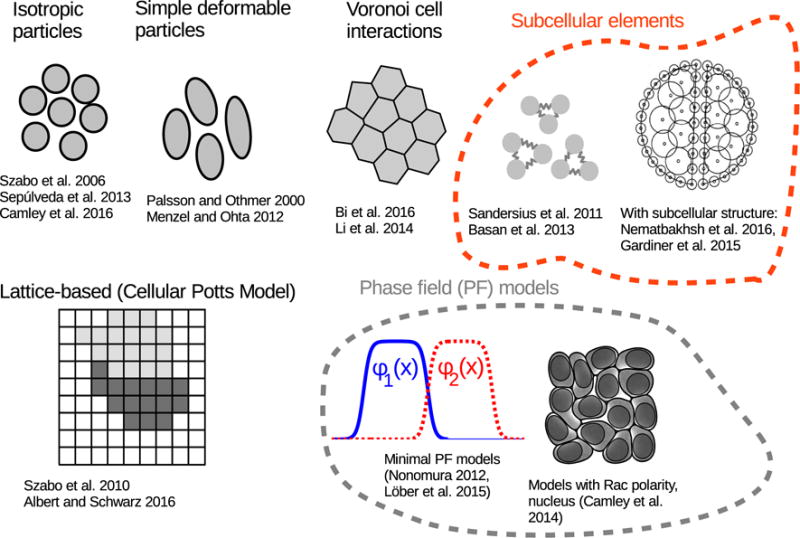
We show illustrations of isotropic particles [39, 13, 17], simple deformable particles [64, 61], Voronoi models [65, 66], subcellular element models both composed of relatively simple particle-particle coupling [67, 45] and more complex models with subcellular structure [68, 69] (the figure shown is from [68]), cellular Potts models [42, 70], and phase field models [71, 72, 34]. These references are not necessarily the first uses of the models; we have highlighted papers we find interesting and relevant.
Isotropic particles
A standard representation of cells is of interacting isotropic particles. If the cells are considered to be overdamped, a typical way to write this would be to describe the equation of motion for cell i’s center of mass, writing Newton’s equations with zero acceleration:
| (3) |
Commonly, is chosen as a frictional force, Factive is the motility force (e.g. p in Eq. 1), and
| (4) |
The potential U is generally constructed of a pairwise interaction, with V having a short-range repulsion and a longer-range attraction, as in molecular dynamics. The origins of these terms is very different than in molecular systems! The effective short-range repulsion arises from an exclusion of cell-cell overlaps, while attraction represents a cell’s adhesion to its neighbor. However, if this is representing a physical attraction, it is mediated by, e.g. cadherins on the cell surface, and should be relatively short-range. Generic models of self-propelled particles with long-range interactions [73] may not be as appropriate to describe cells interacting without long-range chemical secretions.
Choosing in Eq. 3 is a common, but not universal choice. This is a friction appropriate to low-Reynolds number flow relative to a substrate or extracellular matrix – the friction is proportional to the velocity relative to a fixed background. Frictional forces between cells may also be modeled, which will depend on the relative velocities of contacting cells, e.g. vi−vj [74, 64]. A more complicated friction based on dissipative particle dynamics has also been applied [45].
We also note that interactions beyond simple pairwise potentials have been included in several recent papers; these interactions do not necessarily correspond directly to a many-body potential, but are included as the equation of motion Eq. 3. These terms are often used to alter the dynamics of cells at the boundary of a tissue. For instance, [75] include a term for cells at the boundary to point toward the bulk of the tissue, which can be used to promote cohesion in the absence of cell-cell adhesion. Tarle et al. describe a tissue with explicitly included curvature-dependent forces on the border of several types [76]. We have also recently simulated cells with a many-body term designed to promote cell-cell cohesion, by modulating cell-cell interactions as a function of density [17]; this idea is adapted from studies of liquid-gas coexistence in dissipative particle dynamics [77]. Some aspects of these terms could be considered as natural consequences of simulating cell motion without including the details of cell shape – “integrating out” variables is known to create effective many-body interactions within equilibrium molecular dynamics [78].
Isotropic active particles are an appealingly minimal choice for collective cell simulations where cell shape is not resolved. However, even if no explicit coupling between cell shape and cell behavior is expected, isotropic models can fail to predict how tissue mechanics depends on cell-cell adhesion and density – most strikingly in the recently-studied unjamming transitions in confluent monolayers [79, 62, 63]. This suggests that, at least near the jamming point, we should be cautious in applying and interpreting models that do not resolve cell shape.
Active particles with simple shape deformations
The simplest step beyond considering cells as completely isotropic particles is to include shape at a minimal level, e.g. allowing small deviations from circularity/sphericity. This approach was taken early in models of Dictyostelium [64, 80, 81], where cells were represented by deformable ellipsoids of constant volume. More recent papers have also applied simple deviations from an isotropic cell shape. This includes [61], who parameterize the cell shape by a tensor , where is the axis of deformation and s a measure of the distortion. Others have implemented more detailed quasicircular cell shapes, including [82], who model cells as circular with stochastically forming protrusions spiking out of the cell and [60], who describe the cell shape as a polar function R(θ).
Cell-cell interactions in these models can be complex. The models of [64, 80] phrase the interaction between the ellipsoids as a function of the distance between cell surfaces, which is a natural generalization of the central forces applied in simple isotropic cell models. However, this is not the case for the models of [82, 60], in which cell protrusions are collapsed by contact.
These models are immediately valuable to the study of potential shape-motility couplings, but may share some of the downsides of isotropic particle models. In particular, it is not yet clear if the jamming transition [79, 62, 63] can be properly captured in models with simple ellipsoidal shapes. We also suggest that the models in this section may be most interesting when studying experiments that include both subconfluent and confluent layers of cells, as in [82] – for purely confluent tissues, vertex and Voronoi models may be more appropriate, as we discuss below. We do note, however, that [83] have recently combined a vertex model with their cell-protrusion model of [60].
Voronoi models and vertex models
The active particle descriptions discussed above are a good fit for systems where cells may exist both individually and within collectives, e.g. a monolayer below confluence. However, for cells in a confluent layer, it is often valuable to describe the cells by the geometry of their boundaries (Fig. 2). It is then possible to model the energetics of the cell-cell interfaces, using terms such as [84, 65, 66, 85]
| (5) |
where Ai is the area of a cell and Pi its perimeter. This coarse-grained energy describes cells with a preferred area A0 and preferred perimeter P0. Both vertex and Voronoi models can be described with Hamiltonians of this or similar forms. Active driving of cells can occur through regulating the contractility of different cell-cell junctions [86], or through active forces [65, 66].
The key distinction between vertex models and Voronoi models is the representation of the equation of motion of cells: in a vertex model, the cell is represented directly as a polygon, and the equations of motion of these vertices are written by a force balance as in Eq. 3. In a Voronoi-based model, equations of motion are written for the cell center, and a cell’s shape is defined as the Voronoi neighborhood of its center, i.e. the set of points that are closer to the cell center than to any other cell’s center. This is often appropriate for describing cells within a tissue [87], though it does require that cell shapes are convex polygons. This shape may then feed back on the motion of the cell center, e.g. through forces derived from an energy like Eq. 5. Voronoi models then avoid many of the problems associated with handling element re-arrangments in vertex models [88], though they are more limited in the shapes they can represent. Moreover, models that derive the cell area from the Voronoi neighborhood of the cell center do not have a straightforward and natural way of implementing a free boundary, as the cell edge is only defined in reference to the presence of a neighbor or exterior boundary. Therefore, the Voronoi models of [65, 66] are more easily implemented in completely confluent sheets in periodic boundary conditions or confinement.
Many aspects of vertex models are reviewed and compared in [88, 89]; we have only sketched the barest surface of this topic. We also note that other models use Voronoi tesselations to describe the shape of cells, but do not derive their forces from an energy of the type in Eq. 5 [90]. In these models, the Voronoi neighborhood directly influences the cell’s motion only through determining which cells are neighbors, and cell-cell interactions depend only on the center-center distances.
Subcellular element models
Subcellular element models [91, 92, 67, 68, 69, 45] are, in a sense, a straightforward generalization of the single-particle modeling of cells: instead of being modeled as a single unit, each cell is described as several interacting particles (Fig. 2). Then, instead of merely specifying a cell-cell interaction U(r) as described for center-based models in Eq. 4, it is necessary to describe both inter- and intra-cellular interactions Uintra(r), Uinter(r). Active forces in these models can be handled either as motility forces, as in simplified models [45], or through differential rates of breaking and re-forming of intracellular connections at the cell front/back [67]. Recent models have also extended this approach by modeling the cell membrane and interior separately [68, 69].
Subcellular element models have the distinct advantage that they can capture some of the details of single-cell response to forces e.g. power-law rheology [92], and are therefore a natural starting point for studying the mechanical behavior of cellular aggregates and tissues. However, the consequences of single-cell rheology for larger-scale flows remains mostly uncertain, and it is not clear when the full mechanics of the cells are required to capture reasonable qualitative or quantitative collective behavior.
Cellular Potts models
In cellular Potts models, initially introduced by Glazier and Graner [93, 94], cells and their environment are represented by a lattice with “spin” or “cell id” values at each site. As shown in Fig. 2, cell 1 is defined by the region of the lattice where this spin is equal to one. In this case, the cell’s energy can be written in terms of the interactions between these spin values:
| (6) |
where the first sum is over all pairs of neighboring sites in the lattice. Jab is the energy of interaction between these sites – which could depend on the cell types or other details. The term 1 −δσ(a),σ(b) indicates that two sites with the same spin value σ (i.e. two sites belonging to the same cell) do not have an energy cost for being next to one another.) Ai is the area of cell i, i.e. the number of sites it takes up, and Ai,0 is a target area for that cell; λ penalizes deformations from that area. Jab usually takes on one of a small number of values. For instance, in simulating the sorting of initially mixed cells of two types (“dark” and “light”), several energies are specified: Jdd, the interaction energy between two sites on different dark cells, Jdl the energy for dark-light interactions, Jll, for light-light interactions, and the cell-medium interactions Jlm and Jdm. Here the medium is the region of the lattice not occupied by cells. Depending on the relative strengths of the five energies Jdd Jdl, Jll, Jlm and Jdm, cells may either segregate or mix [93, 95].
This model is typically evolved forward in time by making attempts to copy the spin from one lattice site to a neighboring site, accepted with a probability dependent on the change in energy this change would make, e.g. min(exp(−ΔH/T), 1), with T an artificial temperature, which will control the fluctuations around the equilibrium state.
Many extensions to this approach have been made, including the incorporation of biochemical signaling mechanisms, chemotaxis, alternate updating rules, more detailed modeling of cell-cell adhesions, and subcellular compartments [96, 97, 98, 99, 44]. In particular, we should note that terms that bias the motion of the cells in a particular polarity direction p can also be introduced [43, 42]. This can be done by adding a term proportional to −pi · Σa ra to the Hamiltonian for each cell i, where ra is the vector from the center of mass of cell i to site a. This term promotes the protrusion of the front of the cell, where the vector r is aligned with p, and the contraction of the back.
The CPM is a well-established and extensively studied modeling tool, with many freely available implementations [100, 101]. Its relative computational simplicity allows for large numbers of cells to be simulated, even on a single CPU, even though the CPM resolves cell shape in fluctuating detail. These advantages make it one of the default models for describing collective cell migrations. However, there are some significant drawbacks to the model. Because its evolution occurs through Monte Carlo steps rather than an equation of motion derived from Newtonian laws, time is not well-defined in the system, and interpreting a cell’s motion in terms of forces can be difficult. For this reason, additional modeling is needed in order to reconstruct the traction forces from cell simulations [102, 103, 104]. This is in contrast to, e.g. subcellular element or active particle models, for which traction forces can be derived straightforwardly [46, 47]. In addition, the CPM has been criticized because its central assumptions require fluctuations in the cell boundary in order to move; this creates links between cell mechanics (e.g. cell-cell adhesion or area modulus) and cell motility that may not be realistic [105].
Phase field models
A more recent approach, developed by our group and others [34, 71, 72, 106], is to model cell shape in collective migration via phase fields. Phase fields are a standard technique to represent moving-interface problems by representing an arbitrary region by a field ϕ(r) that smoothly transitions between zero outside of the region and one inside the region. This technique has been applied to describe the motility of single cells by many groups [28, 29, 27, 107]. In a multi-cell context, each cell i is given a phase field ϕ(i). Both single-cell and cell-cell energies can be included in a Hamiltonian form. In the model of [34, 59], the equations of motion for the phase field arise as a minimization of the Hamiltonian, with added active terms arising from the motility of the cell, i.e.,
| (7) |
ζ is a friction coefficient and ε the phase field width. Here, vactive is the velocity due to active driving at the boundary, which can be set by a number of rules. These include choosing the active velocity to be constant and in a direction corresponding to the cell’s polarity [106], or to be normal, with a magnitude set by biochemical polarity within the cell [34]. Many terms could be included in this sort of Hamiltonian, but in the past models have included terms such as H = Hsingle + Hcell−cell, with the single-cell energies given by a Canham-Helfrich energy for the membrane [108]
| (8) |
where ε is a parameter characterizing the phase field’s interface width. The Helfrich energy is a widely-applied model for the energetics of a deformed fluid membrane. The first term is an energy from tension on the membrane, which leads to the interface tending to shorten; γ is the tension. The second term is the bending energy, which is an integral of the (mean) curvature over the membrane, with κ the bending modulus of the membrane. Terms nonlinear in the cell perimeter can also be straightforwardly included [59]. The cell-cell interactions are given by
| (9) |
where the first term penalizes the overlap of two cells (as ϕ is only large in the interior of the cells), and the second term promotes adhesion of the cell boundaries (where ∇ϕ is large).
Phase field models have the advantage that they can be readily integrated with reaction-diffusion mechanisms, and can model energies that include higher-order terms like the membrane’s bending energy. However, they have a high computational cost, as a different PDE must be numerically solved for each cell. In [34, 59], we reduce this cost by only solving the PDE near the cell, as also performed by [71]. Another possibility to improve performance is to extend techniques with multiple phase fields that have been applied in modeling grain growth [109, 110], where the number of phase fields can be reduced by judiciously combining multiple fields into one. [111] have also recently developed a simplified model that solves a single phase field crystal equation to represent all of the cells; this may represent an interesting compromise between the full detail of phase field models and continuum models of many cells.
We view the phase field approach as a valuable framework that can incorporate a broad range of submodels – a modular approach highlighted by [112]. We argue for its use in the simulation of relatively small (< 100) collections of cells, where investigators are interested in the relevance of simultaneous couplings between biochemistry, cell shape, and mechanics.
2.3. Polarity mechanism: how cells choose their direction
A central aspect of any model is its explicit or implicit polarity mechanism – the rules that set how a cell chooses the direction it would like to go – e.g. the active force term p in Eq. 3. We want to emphasize that this is separate from the direction in which the cell actually travels, which can be influenced by the forces applied to the cell. In many cases, we can describe the polarity direction as a vector p. How does a cell decide where it wants to go? This can be as simple as saying that the polarity p is a persistent random walk, as in [65, 106], or include simulations of the biochemical mechanisms of cell-cell signaling and internal protein distributions within the cell, as in [34].
We suggest two broad categories of these mechanisms (Fig. 3): cell-autonomous polarity mechanisms, in which the cell integrates information about itself, and non-cell-autonomous mechanisms, where cells integrate information from other cells. A classical example of a cell-autonomous mechanism is velocity alignment [39, 113, 40], in which a cell’s polarity orients itself to its own velocity. Physical interactions between cells mean that one cell’s velocity is influenced by the presence of other cells – and the end result of this effect can lead to cells aligning with one another. A common non-autonomous mechanism is neighbor alignment, in which cells orient to follow the velocities of their neighbors [114, 115]; this generic type of mechanism is also referred to as “Vicsek alignment” or “flocking.” Unfortunately, the term “velocity alignment” can be ambiguous – does it mean aligning to a cell’s own velocity, or a neighbor’s velocity? In fact, neighbor alignment is also sometimes referred to as velocity alignment [37]. To be completely clear about this distinction, we will use “self alignment” instead of velocity alignment. This also includes the possibility that a cell’s polarity aligns to its displacement [42], which is qualitatively similar to velocity alignment.
Figure 3. Examples of common polarity mechanisms.
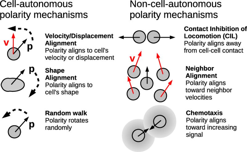
Full explanations of these mechanisms and examples of simulations that use them are listed in the text.
We briefly mention papers that apply these different types of polarity mechanisms, highlighting potential differences in the mechanisms applied; some papers have, either implicitly or explicitly, more than one mechanism.
Self-Alignment and Velocity Alignment
In some early models of collective motion which we now categorize as self-alignment, the polarity of a motile cell is simply reoriented to follow its velocity [39, 113], leading to cells becoming aligned and developing strong collective behaviors, including spontaneous persistent rotation. Many variants of this approach have been developed. In particular, we highlight [42, 18], who apply a self-aligning mechanism to the cellular Potts model. As motions in the cellular Potts model occur through sudden changes in the boundary distribution, the velocity of a cell does not have an unambiguous value without specifying the time (number of Monte Carlo steps) over which the velocity is averaged. In consequence, both Ref. [42] and Ref. [18] effectively align a cell’s polarity toward its past displacement, measured over a timescale T. This has an important distinction from the velocity-aligning models applied in [39, 113] and later studied in other contexts [116, 40]: altering the characteristic timescale of the alignment T will, in the displacement-alignment models, change the persistence of individual cells. This is explicitly studied by [42]. Interestingly, this consequence of displacement alignment is also implied by models generated by detailed tracking of human keratinocytes [36], as [42] notes. More recent papers have applied both velocity alignment and displacement alignment [70, 117, 66, 118, 119]. A related model of “mechanotaxis” has been used by [67], in which cells polarize in the direction of the time-averaged net force exerted on them. These mechanisms are also occasionally integrated with others: [120] and [47] both combine displacement alignment with a model of contact inhibition of locomotion, a mechanism further detailed below.
Unfortunately, in comparing these papers, many model aspects have been varied at once, making it difficult to determine the crucial influence of each element. For instance, one potentially interesting difference between many of these papers is the different origins of noise. In the velocity-alignment model of [39], the cell’s polarity angle θ, i.e. p = (cos θ, sin θ), relaxes to the direction of its velocity θv, but with an added fluctuating Langevin noise in the angular dynamics. By contrast, in cellular Potts model systems, the polarity is set directly by the displacement of the cell, with no added noise [42, 18]; fluctuations arise from the evolution of the cell boundary, leading to fluctuations in the displacement. An extreme case of noisy dynamics in a self-aligning model is our approach in [45, 46, 47], where cells switch between a motile state and a non-motile state with a rate that depends on the alignment between the cell’s polarity and (averaged) velocity. Here, a cell’s orientation is completely randomized upon repolarization – but the bias in the rates still leads to a feedback between flow and polarity. Comparing these various options within a single unified framework would be a potentially valuable contribution.
Self-alignment mechanisms are a reasonable phenomenological suggestion for driving collective cell migration, leading to coordination without requiring any explicit cell-cell communication. However, they may be in conflict with experiment in some circumstances; [121] observe that cells encountering a physical barrier halt, and do not reverse as predicted by a velocity alignment mechanism [40]. In these cases, mechanisms specific to cell-cell contact, e.g. contact inhibition of locomotion (described below) may be relevant.
Shape Alignment
In models that resolve the cell’s shape, the cell polarity can be directly influenced by the cell shape – and thus cell-cell collisions and collisions between the cell and objects can reorient polarity. This is perhaps most explicitly modeled in the minimal approach of Ohta et al. [122], who study the dynamics of a deformable self-propelled particle, and have later extended this to describing the dynamics of Dictyostelium cells [123]. In the simplest version of their model, cells are described by a velocity v and a single tensor variable Sij indicating the cell’s shape deformation from a circle [122]; the most general equations of motion coupling v and Sij to a given order can then be written down. These models, though very minimal, can provide insight into dynamics of single cells, including a turning instability we found in a model with a more complicated, biochemical polarity mechanism [124]. When the single-cell model of [122] is extended to study multiple cells, where cell-cell interactions create deformations, solely the physical cell-cell interactions and the coupling of shape to cell velocity create collective motion, including long range alignment, laning, and nematic alignment, depending on cell density, aspect ratio, and the strength of cell-cell exclusion interactions [61]. A similar effect is modeled in [60], in which Coburn et al. describe cells with a lamellipodium that collapses on contact, with these collapses changing the cell’s directionality. A minimal variant of this sort of model, in which cell motility is proportional to cell length, has also been proposed recently by Schnyder et al. [125].
Contact Inhibition of Locomotion (CIL)
Of the polarity mechanisms we discuss, CIL is the most biologically well-established, both in vitro and in vivo. Many cell types are known to repolarize and reverse upon contact, and many potential biochemical regulators of this process are known. See [126, 127] for recent reviews. However, modeling of this process is at an early stage, and there are many distinct schemes created to model CIL. These include cells developing a bias in polarity away from cell-cell contact [128, 17, 38], rotation away from cell-cell contact [41], collapse of contacting lamellipodia [60] (also an example of shape alignment), and explicit models of biochemical signaling arising from a generation of a Rac inhibitor at cell-cell contact [34, 59]. The models of [120, 47] both combines a CIL bias away from contact with self-alignment.
These subtle differences in modeling can create vastly different results. For instance, the models of CIL in [128, 17, 38], where cells are repolarized away from cell contact, do not develop a spontaneous collective polarity, and would not move in a directed fashion in the absence of a guiding signal. By contrast, [41], who model CIL as an active rotation away from contacting cells, observe spontaneous polarization and flocking, with cells moving in a coherent group despite the absence of any signal beyond confinement. This difference may not be solely due to the CIL model, though, as [41] also includes a long-range attraction from chemotaxis and a term tending to restore cells to constant speed; a similar combination of effects can result in spontaneous polarization as well as rotating vortices even in the absence of explicit aligning effects [73]. Our group has also focused on the consequences of small changes in biochemical CIL models [34, 59]. The behavior of cell-cell collisions and collective rotations can depend critically on whether CIL occurs at all points along the cell-cell contact or merely at the cell front; details of when during the cell-cell collision process CIL begins can also significantly alter the collision outcome. We will discuss these results in more detail in Section 3.1.
Neighbor alignment
Classical models for macroscopic animal herding or flocking invoke neighbor alignment, where animals look to their nearest neighbors and align their motion to what they see [129, 130]. Similar approaches have been proposed for cell motility, leading to collective behaviors such as vortex formation and high coordination in good agreement with experiments [115, 43, 13]. However, we know of no experiment indicating that feedback between cell velocities is occurring, and we note that the neighbor alignment mechanism does not produce reasonable results for pairs of cells rotating on a micropattern [34]. Nonetheless, the good agreement between theory and experiment at large scales [13] suggests that some large-scale effects may not be sensitive to the details of cell-cell interaction, and that neighbor alignment can be a reasonable effective interaction.
Chemotaxis
Cells may, of course, be oriented by signaling beyond direct cell-cell contact or alignment to nearest neighbors. One example involves following a chemical gradient imposed either externally or by cell neighbors. We will discuss this more in Section 2.4 below, and chemotaxis will play a large role in some of the studies we discuss in Section 3 as well.
Implicit alignment mechanisms
Even without explicit mechanisms designed to alter the cell’s polarity as a function of its shape, neighbors, or velocity, many collective cell migration models develop emergent aligning effects. We note, e.g., [72, 131], who have both found that extending a detailed single-cell model to study cell-cell interactions can lead to an emergent aligning effect. These effects may well arise from an effective coupling between cell shape and directionality. In support of this idea, we have demonstrated that cell shape may have important effects on reorienting cell polarity within a single cell model coupling reaction-diffusion equations with a deformable cell shape [124]. However, we caution that these aligning effects may depend on the details of the single-cell model: in [34] we found that merely confining pairs of interacting cells did not lead to robust collective motion without an explicit polarity mechanism.
2.4. Chemical signaling and cell-cell variation
One of the key distinctions between minimal active matter and collective cell migration is that cells in a tissue may communicate chemically, and that different cells in tissue may have different phenotypes. We highlight ideas and common motifs that are particularly relevant for controlling the dynamics, coherence, and directionality of collective migration in Fig. 4.
Figure 4. Common motifs in chemical signaling and cell-cell variation in collective migration.
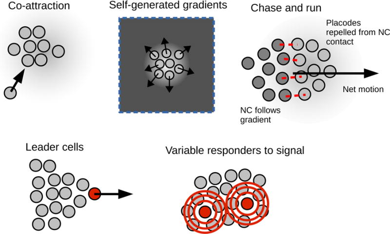
Cell-cell signaling and distinctions between cells with different phenotypes can be relevant in collective cell migration. More details for each of these motifs are provided in the text.
Many applications of collective migration naturally involve chemical signaling and chemotaxis, including wound healing [132, 133], cancer [134], and development [9, 135]. In particular, we mention two means by which collective migration may be controlled by signals generated by local cells: co-attraction and self-generated gradients.
Co-attraction
If cells secrete a signal that they also chemotax toward, cells tend to move up the cell density gradient, and thus aggregate (Fig. 4). This co-attraction, and related mechanisms of signal relay, are known to function in neural crest, Dictyostelium, and neutrophil chemotaxis [136, 137, 135]. Co-attraction is a typical mechanism to mediate aggregation and cohesion of a group of cells, especially ones like neural crest that lack strong epithelial-like adhesion.
Self-generated gradients
In contrast to co-attraction, which supports aggregation and coherence of cell clusters, self-generated gradients can be used to create efficient dispersion or directed migration of a cell cluster. If cells degrade or segregate a chemoattractant or chemokine, a gradient of that signalling molecule will be generated, increasing away from the bulk of the tissue (Fig. 4), leading to efficient outwardly-directed motion [138, 139, 140, 141, 142, 143].
Cells of different phenotypes may also play a large role in collective migration (Fig. 4). A critical example of this is the role of leader cells in wound healing and development [7, 13, 144, 145]. In wound healing experiments, some cells at the border appear to take on a different phenotype, with a larger size and highly active lamellipodium [7]; these cells may then lead to the generation of fingerlike protrusions [13] being guided by these leaders. Cranial neural crest migration can also be modeled by assuming that only leader cells follow VEGF gradients [144, 145], and a similar leader-follower dynamic may be relevant in the zebrafish posterior lateral line primordium [146].
Not all of the relevant phenotypes are as simple as “leader” or “follower.” For instance, Dictyostelium cells show a highly varied set of responses to chemoattractant exposure (Fig. 4), which may increase their ability to aggregate [147]. An interesting combination of the coexistence of different cell types and chemical signaling in collective cell migration is the chase-and-run mechanism [148, 149] in which directed motion arises from the coexistence of two cell types (Fig. 4). Theveneau et al. [149] have shown that neural crest (NC) cells “chase” a population of placodal cells by following a chemoattractant (Sdf1) secreted by the placodal cells. Placodal cells have a contact-dependent repulsion from neural crest cells, leading to a net migration.
3. Specific examples
In this section we will highlight some of the more recent modeling efforts in collective cell motility with a special focus on the different insights that simple (e.g. self-propelled particle) or more complicated (phase field) models can provide into the fundamental mechanisms of group motion. Our choice of models is biased towards our own work but we attempt to put these into a broad modeling and experimental context. We will start with examples of collective motion that involves a small number of cells and conclude with simulations of large confluent cell sheets.
3.1. Motion on micropatterned surfaces
In vivo cell motion is challenging to visualize and quantify and typically involves 3D motion through complex environments. A standard experimental way to simplify the extra-cellular environment is to investigate cell motion on flat substrates, thus constraining the motion to 2D. A further simplification can be realized by micropatterning the substrate, creating adhesive domains that are surrounded by non-adhesive surfaces. Cells are thus constrained to the micropattern, not only facilitating visualization but also enabling the experimentalist to probe the effects of containment. Furthermore, the relative low number of cells permits the use of modeling studies in which cell shapes can be dynamically altered [150].
One of the simplest examples of the use of micropatterns in motility research comes from studies of pairs of endothelial cells on islands of fibronectin. These pairs were observed to robustly develop persistent rotational motion (PRM) in a yin and yang like shape, as shown in Fig. 5A [151, 152]. In contrast, fibroblasts did not rotate, developing a straight, static interface between the two cells, demonstrating that cell specific mechanisms are responsible for the observed motion. Leong addressed the motion of two cells in a square geometry using a dissipative particle dynamics model [153]. In this model, the two cells were permanently attached and developed PRM with shapes that were consistent with the experiments. However, the cells did not contain a nucleus, potentially important for determining the cell’s shape, and a single cell did not have a clear polarity.
Figure 5. Collective motion on micropatterned substrates.
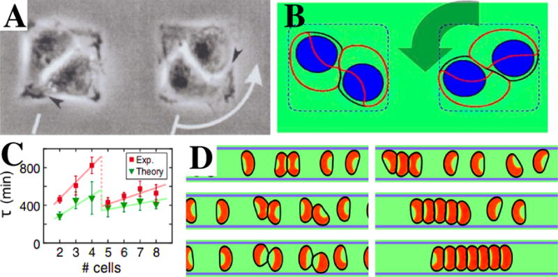
A. Collective motion of two cells on a square 40 μm× 40 μm fibronectin-coated adhesive island, with arrow indicating the direction of motion. (From [152]). B. Example of a rotating pair on a micropattern with dimensions 30 μm× 30 μm obtained using the phase field [34]. The cell membrane is indicated by a black line, the polarity protein by a red contour, the cell nucleus by a blue shape, and the micropattern by a blue dashed line. C. Persistence time τ as a function of the number of cells on a circular micropattern. Note the sharp drop between 4 and 5 cells, attributable to the geometric rearrangement of cells (From [154]). D. Examples of simulated cell motion on a 1D stripe. Depending on model parameters, cells either continuously reverse direction following a collision (left three panels, time going down), or form a chain of cells (right three panels). Adapted from [59].
In a separate study, we modeled this simple collective migration using the phase field model [34]. Cells were modeled as objects with a preferred area and containing a nucleus, exhibiting cell polarity, and exerting forces on the substrate and on neighboring cells. Four different cell polarity mechanisms were included and their effect on rotational motion was studied. Three of these mechanisms were already discussed in Section 2.3: neighbor alignment, velocity alignment, and CIL (contact inhibition of locomotion). In addition, we included cell front-front inhibition, a generalization of CIL in which only contact with the cell front is inhibitory, was included. Implementing these different mechanisms revealed that collective migration is highly sensitive to the polarity mechanism. Specifically, only the velocity alignment mechanism robustly promotes the presence of PRM while the front-front inhibition only allows persistent rotation if cells are sufficiently confined (Fig. 5B). Furthermore, our study revealed that, in addition to a polarity mechanism, PRM also requires that the cell’s linear motion be sufficiently persistent and that cells that undergo pure random-walk motility are not likely to develop rotation. The prediction that collective motion depends sensitively on persistence might be experimentally testable by altering known modulators of cell persistence [155, 156]. Furthermore, the study showed that the nucleus can have an important effect on the shape of the cell-cell interface. This prediction can also be tested experimentally, by studying cells with smaller or no nuclei [157].
In additional studies, collective migration of cells restricted to larger circular domains was investigated [154, 158]. The experiments, using Madin-Darby canine kidney (MDCK) cells, showed that for small enough circular domains, cells rotated in a coherent fashion [158]. Similar vortex-type motion has also been observed in other cell systems even in the absence of confinement, where only cell-cell adhesion is sufficient for coherent motion [159, 160]. In even smaller sized circular domains, clusters of MDCK cells alternated between states of disordered motion and states of coherent rotational motion [154]. The time spent in the coherent state was measured as a function of cell number and showed a pronounced drop between four and five cells (Fig. 5C), attributed to the difference in cell arrangement (a conformation without a cell in the system center vs. one including a centered cell). These experimental findings were addressed using a cellular Potts model (CPM), as described in Section 2 [93], generalized to include internal polarization. The model distinguishes between protrusions and retractions and couples the local dynamics of the internal polarization field to the cell’s protrusions. This coupling produces a positive feedback between intracellular events and mechanical stimuli and results in spontaneous polarization. After carrying out a parameter sweep, Ref. [154] found that the model can replicate the abrupt drop in persistence time for the rotational state when the cell number is increased from 4 to 5 (Fig. 5C). As in the experiments, this drop could be attributed to the geometric rearrangement of cells: the confirmation changes from no cell to a single cell at the center of the pattern. Thus, the model showed that a coupling between cell polarity and cell-cell interaction is sufficient to explain the experimental results.
A final example illustrating how models can shed light on cell-cell interaction mechanisms involves the motion of cells on 1D stripes [161, 162]. Recently, micropatterned substrates which contain 1D adhesive regions have been used to study what happens when cells collide [121, 163, 164, 165]. By restricting cell motion to the stripe, these experiments can efficiently generate collisions under consistent conditions. Experiments of head-on collisions of neural crest cells revealed that the majority of cell collisions resulted in cell reversals: after the collision, both cells reverse their direction [163, 121]. Some cell pairs, however, stuck together after the collision or, in rare cases, walked past each other. Importantly, these experiments were carried out for a sufficient number of collisions to generate quantitative statistics.
The results of the collision assay can be compared to the outcome of models with different potential mechanisms of cell-cell interactions, as we did in a recent study using the phase field method [59]. In this paper, we described cells crawling on a quasi-one-dimensional narrow adhesive stripe, and the deformable cells were given a polarity using a model which describes the dynamics of a polarity protein, assumed to be Rac [24]. CIL was implemented by assuming that cell-cell contact results in the production of Rac inhibitor as in [34]. The inhibitor field was assumed to include fluctuations, rendering the simulations st ochastic. For each set of parameters, we simulated a large number of head-on collisions. These simulations were able to reproduce all experimentally observed outcomes but, as we have already seen in the case of the rotating cell pair on the micropattern, the outcomes were sensitive to the precise values of the parameters like the rates of inhibitor generation, the asymmetry of CIL between front and back, and the cell-cell adhesion strength. This is also evident when multiple cells are placed on the stripe, as was also carried out in a recent experiment [121]. For model parameters that favor cell reversals, cells collide and reverse direction, without forming clusters of more than two cells (Fig. 5D). Changing the parameters such that they promote chains, on the other hand, result in a single and persistent train, as observed in the experiments [121, 166].
3.2. Collective chemotaxis
One of the most striking examples that demonstrates that collective motion is not merely the sum of the motion of many single independent cells comes from the field of chemotaxis. Here, a chemical gradient results in an asymmetric distribution of bound receptors which leads to the directed motion of cells up the gradient‡. Chemotaxis is believed to play an important role in would healing, as well as embryogenesis and, possibly, cancer metastasis [134, 167]. For reviews on single cell chemotaxis we refer to [168, 169, 170]. It has long been known that clusters of cells can chemotax as well [171, 172]. Recent experiments, however, have shown that single cells and clusters of cells can have dramatically different behavior when placed in a chemoattractant gradient. For example, and illustrated in Fig. 6A, the motion of clusters of lymphocytes was shown to migrate directionally and to better follow chemotactic gradients than individual cells [16]. In fact, these lymphocyte clusters always followed the gradient, independent of its steepness, while single cells reversed directionality for very steep gradients. Clusters of neural crest cells were also shown to be attracted toward sources of chemokines while single neural crest cells did not show any directionality in their movement [15]. Similar examples of emergent taxes have been observed in electrotaxis of epithelial sheets [173], durotaxis of epithelial sheets [174], and chemotaxis of Myxococcus xanthus swarms [175]. These surprising findings clearly highlight the effect of multiple cells on motility. (We also note, at a much larger length scale, emergent phototaxis of fish schools [176].)
Figure 6. Chemotaxis of clusters.
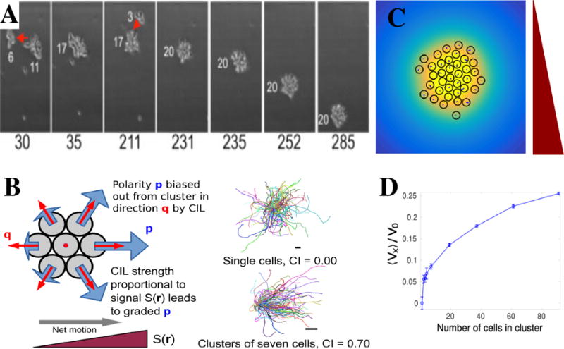
A. Lympocyte cells respond to a downward gradient only if the cluster has a sufficient size. Shown here are snapshots at times indicated (minutes); smaller cell clusters merge and form a larger one which migrates downward (From [16]). B. Schematic representation of the model of Refs. [17, 38]. CIL is incorporated by assuming that the cell’s polarity p is biased toward the vector q which is proportional to the average over the positions of the cell’s neighbors and points away from the cluster. The strength of this bias is regulated by the local chemoattractant value S(r), leading to cells being more polarized at higher S. As a result, single cell trajectories show no bias towards the gradient direction while a cluster shows an average direction motion towards higher chemoattractant concentrations. For both cases, 100 trajectories of six persistence times in length are shown. For more details, see [17]. C. Snapshot of a chemotaxing cluster bound by co-attraction that is mediated by a secreted co-attractant field, shown in yellow. The chemoattractant gradient is pointing downward. D. The chemotactic velocity of clusters bound by co-attraction shows a gradual increase as the cluster size increases. Panels C and D are taken from [38].
How can a cluster of cells respond to a gradient while a single cell does not? To answer this question in experiments is challenging. Most likely, cell-cell communication is responsible for the divergence of behavior. This communication can potentially be of different origins. For example, it is possible that cells communicate through gap junctions which allows chemical species to be shared between cells within the cluster [177]. It is also possible that cells secrete chemicals that then diffuse extracellularly and can interact with neighboring cells. Finally, it is also conceivable that mechanics, either through cell-cell contacts or cell-substrate modifications play a role.
One possible mechanism that would explain an enhanced chemotactic ability for clusters would involve cells that each independently sense the gradient, while the cluster has increased accuracy by averaging over many independent measurements. Alternatively, the presence of neighbors could induce cells to change their gradient-sensing behavior – e.g. single cells amplify their response to shallow gradients when exposed to a quorum-sensing factor. The experiments using lymphocytes, however, show that even when single cells move down the gradient, clusters are still able to chemotax up the gradient. Thus, at least for these cells, spatially averaging is not likely the most dominant mechanism, and the mechanisms of single-cell and collective chemotaxis are likely to be fundamentally different.
A number of models have been put forth to explain the difference between single cell and cluster chemotaxis. A recent study was inspired by experiments using lymphocytes which showed that 1) clusters were able to chemotax above a critical size of ~20 cells, 2) the velocity of the clusters was largely independent of their size, 3) the variance of the velocity decreases for increasing cluster sizes, and 4) the forward migration index (FMI) (defined as cell displacement along the gradient direction/track length) increases as cluster sizes increase [16]. In the model, clusters were modeled as 2D circular aggregates [16]. Through an unspecified mechanism, only cells at the perimeter were assumed to respond to the chemoattractant and were assumed to exert normally outward forces, proportional to the local concentration. In addition, cells were able to exert random traction forces. The total outward force along the perimeter in this model scales with the size of the cluster (Fper ~ R2). Assuming that the friction between the cluster and the aggregate is simply proportional the area results in a cluster velocity that is largely independent of its size, as observed in the experiments [16]. For uncorrelated noise, the model predicts that the variance in the cluster velocity scales inversely with the area, 〈v2〉 ~ 1/R2, in good agreement with the experiments. Combining these two findings results in a FMI that increases for increasing cluster sizes and that can be fitted to the experimental results.
We also have recently proposed a model for the emergence of chemotaxis in collective systems, motivated by the experimental results of neural crest cells [15, 178]. In this model, schematically illustrated in Fig. 6B, cells are again modeled as rigid circular objects and clusters as 2D aggregates [17, 38]. A key component of the model is CIL, in which cells move away from neighboring cells and which we described in Section 2.3 [179, 121, 164, 180]. The model assumes that the strength of the CIL is proportional to the local chemoattractant concentration resulting in a spatial bias of cell-cell interaction and cluster chemotaxis. We note that since the gradient only affects cell-cell interactions, single cells will not chemotax (Fig. 6B). Each cell i has a position xi and a polarity pi, which obey a variation of Eqs. 1,2, and 3:
| (10) |
| (11) |
where Fij are intercellular forces of cell-cell adhesion and volume exclusion, and ξi(t) are Gaussian Langevin noises with . Greek indices μ, ν run over the dimensions x, y. The first two terms on the right of Eq. 11 are a standard Ornstein-Uhlenbeck model: pi relaxes to zero with timescale τ, but is driven away from zero by the noise ξ(t). This corresponds to a cell that is orientationally persistent over time τ. The term is our simplest model for CIL – cell i polarizes away from its neighbors j.
The advantage of this model is that it can be used to generate analytical predictions. Specifically, the mean velocity of a cluster can be shown to be [17]
| (12) |
The matrix ℳ only depends on the cells’ configuration,
| (13) |
where . For rigid clusters, i.e. clusters in which the cells do not rearrange, this matrix can be explicitly determined. We found that the mean velocity depends on the orientation of the cluster, its shape and its size. For large near-circular clusters, it can be shown that the velocity saturates as N → ∞:
| (14) |
This can also be understood by realizing that the velocity is proportional to the ratio of the total protrusive forces and the friction forces. The latter should scale as N while the former should scale as the size of the perimeter times the difference in concentration between the front and back of the cluster (also ). These results also allowed for explicit analytical expression for the efficiency of chemotaxis. Furthermore, simulations revealed that the velocity of nonrigid clusters also saturates for large cluster sizes.
In the minimal model described above cells only react to the local chemoattractant concentration. What would happen if cells communicate with each other through chemical signals as we already discussed in Section 2.4? We investigated this in an extension of the model in which cells not only interact with their nearest neighbors but also interact on a longer spatial scale through chemical secretions [38]. Specifically, a local excitation, global inhibition (LEGI) scheme was implemented in which the chemoattractant induces production of a long-range diffusive inhibitor and a local activator [181, 182]. This scheme has been used extensively for single cells and adapts perfectly to changing uniform signals [182, 183]. For very fast diffusion, it was found that the cluster velocity, as in the minimal model, saturates for large cluster sizes. For more physically realistic values of the diffusion rate, however, the cluster velocity depends non-monotonically on the cluster size. In this case, cells cannot effectively communicate across the cluster and gradient sensing becomes non-linear, resulting in a maximum velocity for a finite cluster size. This maximum velocity has also recently been confirmed in a different model by combining a similar LEGI signaling model with the cellular Potts model [44].
Our study also investigated the possibility of co-attraction mediated through chemical secretions, as known to occur in neural crest cells [135, 41]. A snapshot of a simulation of a cluster in which particles secrete a co-attraction species is plotted in Fig. 6C. The additional species is shown in yellow and is assumed to be secreted in equal amounts by all cells, after which it diffuses and decays. As a result, its concentration is highest at the center of the cluster, which is now only loosely bound and displays significant cell re-arrangements. Nevertheless, for suitable parameters, these clusters remain coherent and migrate up the chemoattractant gradient. Interestingly, the velocity of larger clusters does not saturate but continues to increase, as can be seen in Fig. 6D. This can be understood by recalling that in the rigid cluster model the velocity saturates due to a balance of friction forces (~N) and the CIL forces which are exerted on the edge ( cells) and increase linearly with the radius of the cluster . In the case of co-attraction, the CIL forces are no longer restricted to the cluster perimeter but act at any cell-cell collision.
3.3. Modeling cell sheets
In many experimental studies of collective motion, cells are part of large confluent sheets. For example, the commonly used “wound-healing” assay consists of a monolayer of cells that is suddenly able to move into an area void of cells, created either by a scratch [184] or by using more sophisticated methods [7, 185, 186]. Another example includes seeding a confluent layer of cells and observing its growth [187, 188, 189]. These experiments revealed that cells within the bulk display characteristic dynamics, with correlated motion across many cell lengths and swirling motion [7, 187]. Also, fronts that invade empty space often do not remain planar but exhibit an instability resulting in long finger-like protrusions (Fig. 7A) [7, 190]. Finally, by measuring traction forces generated by the cell layers, it was shown that not only cells at the edge of the sheet exerted forces but also cells in the middle of the sheet, many cell diameters away from the boundary [189].
Figure 7. Collective motion simulated by particle-based models.
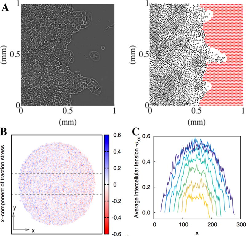
A. Experimental (left) and simulation (right) snapshot of an epithelial cell layer invading a void. The experimental picture is shown 20h after after removing the barrier and clearly shows a finger-like protrusion. In the simulation snapshot, cells are represented as black dots. For further details, see Ref. [13]. B. Snapshot of the x component of the traction stress in a simulation of a spreading cell colony using a two-particle-per cell model [47]. C. Average tension in the x direction calculated by integrating average traction stress along the y axis within the region indicated by dotted lines in B.
Attempting to model these sheets as collections of deformable objects is often computationally too costly, although the cellular Potts model is able to simulate thousands of cells [18]. Continuum models can be used to model the spreading of cell layers but do not always incorporate all observed effects, including cell division and motility forces within the bulk [191, 192]. Particle-based models, in which cells are treated as disks, can provide an attractive alternative to both continuum models and to deformable cell models: they are computationally efficient and allow for the explicit incorporation of specific mechanisms. By introducing cell-cell interactions or by assigning different properties to different cells one can then use these models to investigate potential mechanisms.
In one recent approach to particle-based models of monolayer expansion [13], the cell’s position is described by its center of mass and its velocity obeys
| (15) |
Here, the first term describes dissipative damping while the second term, which represents a sum over all nearest neighbors, incorporates a neighbor alignment mechanism as well as short scale repulsion and long-range attraction (Fij). The neighbor alignment is controlled by the parameter β and incorporates the idea that cells tend to move in the direction of their neighbors, as we discussed in Section 2.3 [115, 193, 160]. The final term represents noise and is typically modeled as a standard Ornstein-Uhlenbeck process. This stochastic particle model is able to reproduce a number of experimental features. For suitable parameters, for example, the bulk display large-scale flows that are similar to the experimental ones. Specifically, a quantitative comparison using different statistical quantities, including the velocity field auto-correlation and distributions of velocities, provided a good match between experiments and models [13, 194]. We note that Eq. 15, unlike our model of Eq. 10–11, does not distinguish between a cell’s velocity and its polarity; therefore, even though the cell’s environment is overdamped, there is an acceleration term on the left hand side of Eq. 15. This should be interpreted as the time required to reorient a cell, and is not related to the cell’s physical mass.
This type of model can be extended in several ways. For example, it is possible to introduce leader cells, i.e. cells that are at the edge of the sheet and that have different motility properties. This extension is motivated by experimental observations that cells at the boundary of the sheet have a distinct morphology [7]. When introducing leader cells that were faster than cells in the bulk and that have a fixed outward predetermined velocity, the model showed a fingering instability consistent with the experiments (Fig. 7B) [13]. In a more recent study, the model was extended even further by adding specific forces at the outer edge of the cell layer, including a surface-elasticity restoring force and a curvature-dependent positive feedback which assumes that cells at convex parts of the front exert larger forces [76]. In addition, a purse-string mechanism was included which describe the experimentally observed actin-myosin cable that can exert large tension forces on the boundary cells [195, 196]. By systematically varying the relative strength of these forces it was possible to determine which mechanism is essential for the fingering instability. [76] discovered that the positive feedback between protrusions and motility is an essential ingredient for the formation of fingers in the absence of explicit leader cells.
A variant of this model using ideas from dissipative particle dynamics has been used to study the properties of 3D tissue aggregates like their growth, competition, rheology, surface tension, cell sorting, and the diffusion of cells within the tissue [197, 198, 199]. In this model, each cell is represented by two interacting particles, one representing the cell front and one the cell back – making this also a variant of subcellular element models, as discussed above. Cell growth is incorporated by setting a maximum distance between these two particles, above which the cell divides. Cells can switch between a motile and a nonmotile state; only cells in the motile state exert a force onto the substrate. An alignment mechanism can be implemented by assuming that the transition rate depends on the orientation of the motility force relative to the cell velocity of the neighbors. Such a model can also reproduce the swirling bulk dynamics with long-range velocity correlations [45]. It is able to reproduce the finger-like protrusion when simulating an invading front, although a systematic studies of the relevant parameters and mechanisms has not yet been carried out.
We have also recently used a cell-pair model [45, 47] to study the closure of circular wounds, motivated by recent experiments [191]. We found that the model dynamics and tissue velocity profiles agree well with the experimentally observed ones [200]. This model also showed that the alignment mechanism can speed up wound closure and the collective migration is sufficient to close circular wounds. Thus, and consistent with earlier modeling work [192, 13], wound closure does not require cell division or a purse-string (active contractile cable at the tissue boundary) mechanism.
Finally, the cell-pair model has also been used to compare simulated traction forces generated to the experimental results of spreading colonies [189]. We found that the stress maps produced in the model agree well with the experimentally determined ones [45, 47]. In particular, significant traction forces were not only present at the edge but existed throughout the entire colony. Furthermore, the model was able to reproduce the build up of tensile stress as observed in the experiments, even though the model did not include leader cells, as illustrated in Fig. 7C and D. Leader cells were also not required to reproduce detailed experimental results of collective motion in epithelial cell sheets [201], suggesting that in some cases collective migration can be achieved without the presence of specialized cells at the boundary. We should also point out that the model was used to validate a procedure of obtaining the intercellular stress maps from measured traction forces on the substrate [202]. The model showed that the stress maps obtained from the simulations are in good agreement with the experimentally determined maps, provided that the traction forces are not too weak, and thus validated the experimental method [46]. This is one of the additional strengths of a modeling approach: stress maps, and other quantities that are not readily available in experiments, can be directly computed and can be used to validate experimental procedures at arbitrary precision.
4. Future directions
What directions can, and should, modeling of collective cell motility take in the future? We highlight a few idiosyncratically chosen paths below.
4.1. Discrimination between polarity mechanisms vs searching for universality
The problems we discuss in Section 3 tend to have two different characters: investigation into the precise methods by which cells interact with each other and sense signals, and the large-scale dynamics of tissues comprised of hundreds of cells. We have found that performing strict tests of specific cell-cell interaction models is often easier with small numbers of cells. Pairs of cells undergoing a neighbor alignment do not rotate, while those using velocity alignment do [34] – but both self- and neighbor-alignment can create rotations of large systems [43, 158]. Similarly, in studying the velocity and directionality of clusters guided by a chemical signal, we found that single-cell gradient sensing and collective gradient sensing mechanisms could produce highly similar results at large cluster sizes – but could be discriminated by studying the behavior of pairs of cells [17].
Under what circumstances, then, should we expect different polarity mechanisms to give similar results? This question of universality has been hinted at in earlier papers [18], but not addressed extensively. One approach might be to study the systematic coarse-graining of models that resolve the cell scale into continuum hydrodynamic equations. Steps have been taken in this direction, both deriving hydrodynamic equations corresponding to minimal models of active matter (e.g. the Vicsek model) [203, 204, 205, 206], and building continuum elastic theories from vertex models [207]. Links between the cellular Potts model and continuum models have also been developed [208]. Additional study in these directions may provide some clarity on the question of universality.
4.2. Resolving important differences: multi-model comparisons on standardized problems
One aspect of modeling collective cell migration that we have tried to illustrate is that in studying a given problem, there are many small decisions along the way which are not necessarily determined by the experimental data. These decisions may not be highlighted in modeling papers, but they can nonetheless be important. These include the level of representation of the cell shape, the choice of polarity mechanism, and the statistics of single cells. A natural way to address this would be to apply multiple simulation methodologies to simultaneously characterize a single modeled behavior, as done in, e.g. [209, 210]. In addition, studying multiple mechanisms simultaneously may be necessary [34]; we should expect that several reasonable explanations can exist simultaneously for cell behaviors (e.g. [211] in single-cell dynamics), and work to propose potential tests to discriminate between them.
We argue that applying several modeling frameworks to a single problem is a valuable first step toward seeing how generalizable a simulation’s results are, determining the generality and robustness of a proposed mechanism, and finding the minimal necessary ingredients for a model. When we use models to make predictions for a biological experiment, we have to translate between changes in simulation parameters and experimental interventions – e.g. assuming that the strength of a cell-cell interaction potential U(r) is proportional to a cadherin expression level. Comparing simulations in two different frameworks is a miniature version of developing experimental predictions, and can highlight difficulties in generalizing simulations. For instance, because cells in the CPM must protrude in order to move successfully, increasing their effective compressibility λ slows the motion of cells, both individually and collectively; this connection between compressibility and cell speed does not necessarily arise in other models. Another potential trouble point in generalizability is characterizing the multiple roles of cell-cell adhesion. We would expect that pairs of cells with increased cadherin expression require force to separate, e.g. a larger cell-cell potential U(r), but increased adhesion also could increase frictional drag when cells move past each other. Comparing models with frictional forces between cells [74, 64, 45] and without can show these contrasting potential roles of adhesion. These questions become even more complicated when mechanical models are combined with chemistry: we found that increasing adhesion strength can have highly counter-intuitive effects on the collision of cell pairs when biochemical modeling of cell polarity is combined with modeling of the cell shape [59]. Comparison between different models is a useful test of robustness, and a good way of discovering hidden assumptions that can be checked experimentally.
We suggest several key questions that could serve as test problems for comparing models, and illustrate them in Fig. 8.
Figure 8. Potential test problems for characterizing differences between models.
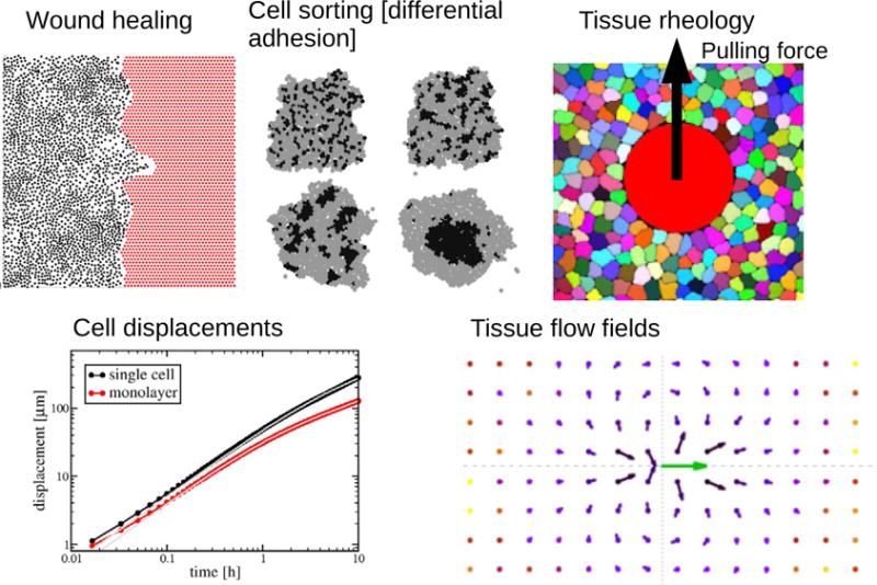
Wound healing illustration taken from self-propelled particle simulations of [13]. Cell sorting image from self-propelled particle simulations of [214]. Active microrheology simulation is from the subcellular element models of [67]. Cell displacements and tissue flow shown from [42].
Wound healing
We have discussed examples of wound healing and tissue expansion in Sec. 3.3 above. We view this as a natural testbed for many different models, given the large amount of experimental data, ranging from the rates of expansion, to fingering instabilities, to the mechanical forces applied on the substrate. In addition, when comparing different modeling approaches, tissue expansion and wound healing has the advantage of many analytical tools developed to better understand the dynamics of the experimental data, e.g. [212, 213].
Cell sorting by differential adhesion
The sorting out of two cell populations arising from a constrast in relative adhesion strengths is one of the classical applications of many simulation methods, including the cellular Potts model [94], self-propelled particle models [214], and many others [210]. This has a broad relevance to the physics of sorting in developmental systems like Hydra regeneration and Dictyostelium spore formation. However, it is also a particularly interesting question for multi-model comparisons, because it depends on many different features: the final state depends critically on the adhesion energies, while the dynamics can strongly depend on both cell-cell alignment and cell motility.
Rheology of tissue
Tissues composed of many cells can be viewed as a complex material, and their mechanical properties like elasticity and viscosity can be studied in this context [215, 216]. Simulation and theory can play a role in understanding the sensitivities and biases of different methods of probing these properties. One particularly interesting approach to measuring tissue material parameters is microrheology [217], in which the motion of small probes are tracked as they move through the material, either by passive thermal fluctuations, or by active probing. This approach has been applied experimentally to tissues [218], though on a shorter timescale than is typically relevant for cell motility and rearrangements. One paper that we know of has simulated the mechanical response of tissue to an active microrheological probe [67]. However, we should mention some caveats in analyzing this sort of data. There are well-established techniques for deriving the linear viscoelasticity of a material to the displacement of a probe driven by a fixed or fluctuating force [217], which require a formula for the mobility of the probe as a function of the tissue viscosity. In a three-dimensional tissue with a spherical probe, this is given by the classical Stokes result: the mobility is μStokes = 1/6πηR, with η the tissue viscosity and R the probe radius. However, in typical two-dimensional simulations and in epithelial monolayers, the relationship is more complex; for a two-dimensional tissue with a cell-surface friction, it is appropriate to apply the Evans-Sackmann mobility [219], which is more complicated, and, depending on the tissue viscosity, can be only logarithmically dependent on the probe radius and on the tissue-surface friction. Ref. [67] applies the Saffman-Delbrück equation [220] to analyze their data, which can approximate Evans-Sackmann in some limits. We also caution that we would expect these quasi-two-dimensional measurements to have strong system size effects, which could be corrected using hydrodynamic theories [221].
Cell displacements and tissue flow
One of the simplest measurements possible to characterize collective cell migration is to look at the displacement of single cells within the tissue, and to compute correlations in these motions [222, 201, 42]. Measuring single-cell mean-squared displacements MSD(t) = 〈|r(t + t0) − r(t0)|2〉 allows the characterization of how persistently a cell can move within a tissue, as well as its effective diffusion coefficient over long times [42]. In addition, calculating the correlation in tissue velocity, or the mean tissue velocity relative to a cell [18, 42] provides a sense of the length over which cell velocities are correlated. These measurements allow for direct simultaneous comparison with experiment and comparison between models [201].
Comparing different models on the same test problem is made easier when code is publicly available. We are aware of many open-source implementations of various collective cell motility models, including vertex models and others in Chaste [88, 210], CompuCell3D [100] and Morpheus [101] for the cellular Potts model, CellSys for center-based models [74] and SEM++ for the subcellular element method [223]. Many other codes are discussed in a extensive review of agent-based methods [33]. We note, however, that these models may not include all of the features we have discussed in this review – in particular, some lack explicit handling of terms like neighbor or velocity alignment or self-propulsion forces.
4.3. Increased mechanical fidelity of cell models
The mechanical response of single cells has been extensively characterized [224], as well as the flow of actin within cells [225]. Some of these elements have been integrated into single-cell models including modeling of the flow of the actin cytoskeleton [29, 211, 226, 227] or application of minimal active fluid models [228], but the impact on collective migration is not yet clear. However, given the clear role of cytosolic hydrodynamics in development [229] and the recent suggestion that some collective cell motility may be limited by hydrodynamic flow in the surrounding tissue [230], extension of models to greater mechanical detail would be highly relevant. An initial step in this direction was recently published by Marth and Voigt, who used collective phase field models to extend a minimal active fluid cell model to handle multiple hydrodynamically-interacting cells [131].
4.4. Role of the mechanical environment
We have mainly focused on the modeling of two-dimensional collective cell migration on rigid substrates. However, in vivo cell migration occurs with strong interactions with the extracellular matrix (ECM). The rigidity and porosity of the matrix is known to regulate motility, while the forces exerted by the cells reshape the matrix [231, 232, 233]. In order to understand collective invasion in vivo, it is necessary to understand this feedback. While the role of the extracellular matrix has certainly been modeled before, especially in developmental biology contexts [234, 103, 235], new techniques in traction force microscopy have highlighted long-range correlations in the stress within two-dimensional monolayers [189]. However, collective cell migration models that reproduce this stress buildup have only recently been developed [47]. Designing models that take the lessons of quantitative traction force microscopy from two dimensions into three is an ambitious, but important goal.
Acknowledgments
We thank Andrew Mugler, Julien Varennes, Dirk Kulawiak, and Albert Bae for careful reading and useful suggestions for this paper. We would also like to acknowledge our many collaborators on the papers on collective cell migration that we discuss here, including Juliane Zimmermann, Herbert Levine, Bo Li, Yanxiang Zhao, Yunsong Zhang, Eshel Ben-Jacob, and Dirk Kulawiak. This work was supported by NIH Grant No. P01 GM078586. BAC was supported in part by NIH Grant No. F32GM110983.
Footnotes
We will restrict ourselves to the case of chemoattractants although chemotaxis in the presence of a gradient of chemorepellants is also possible.
References
- 1.Mitchison T, Cramer L. Cell. 1996;84:371. doi: 10.1016/s0092-8674(00)81281-7. [DOI] [PubMed] [Google Scholar]
- 2.Endres RG, Wingreen NS. PNAS. 2008;105:15749–15754. doi: 10.1073/pnas.0804688105. [DOI] [PMC free article] [PubMed] [Google Scholar]
- 3.Mogilner A. J Math Biol. 2009;58:105–134. doi: 10.1007/s00285-008-0182-2. [DOI] [PMC free article] [PubMed] [Google Scholar]
- 4.Keren K, Pincus Z, Allen GM, Barnhart EL, Marriott G, Mogilner A, Theriot JA. Nature. 2008;453:475–480. doi: 10.1038/nature06952. [DOI] [PMC free article] [PubMed] [Google Scholar]
- 5.Fletcher DA, Mullins RD. Nature. 2010;463:485–492. doi: 10.1038/nature08908. [DOI] [PMC free article] [PubMed] [Google Scholar]
- 6.Jilkine A, Edelstein-Keshet L. PLoS Comput Biol. 2011;7:e1001121. doi: 10.1371/journal.pcbi.1001121. [DOI] [PMC free article] [PubMed] [Google Scholar]
- 7.Poujade M, Grasland-Mongrain E, Hertzog A, Jouanneau J, Chavrier P, Ladoux B, Buguin A, Silberzan P. Proceedings of the National Academy of Sciences. 2007;104:15988. doi: 10.1073/pnas.0705062104. [DOI] [PMC free article] [PubMed] [Google Scholar]
- 8.Clark R. The molecular and cellular biology of wound repair. New York: Plenum; 1996. [Google Scholar]
- 9.Montell DJ. Nature Reviews Molecular Cell Biology. 2003;4:13–24. doi: 10.1038/nrm1006. [DOI] [PubMed] [Google Scholar]
- 10.Dormann D, Weijer CJ. Curr Opin Genet Dev. 2003;13:358–364. doi: 10.1016/s0959-437x(03)00087-x. [DOI] [PubMed] [Google Scholar]
- 11.Friedl P, Gilmour D. Nature Reviews Molecular Cell Biology. 2009;10:445. doi: 10.1038/nrm2720. [DOI] [PubMed] [Google Scholar]
- 12.Cheung KJ, Ewald AJ. Science. 2016;352:167–169. doi: 10.1126/science.aaf6546. [DOI] [PMC free article] [PubMed] [Google Scholar]
- 13.Sepúlveda N, Petitjean L, Cochet O, Grasland-Mongrain E, Silberzan P, Hakim V. PLoS Computational Biology. 2013;9:e1002944. doi: 10.1371/journal.pcbi.1002944. [DOI] [PMC free article] [PubMed] [Google Scholar]
- 14.Tarle V, Ravasio A, Hakim V, Gov NS. Integr Biol (Camb) 2015;7:1218–27. doi: 10.1039/c5ib00092k. [DOI] [PubMed] [Google Scholar]
- 15.Theveneau E, Marchant L, Kuriyama S, Gull M, Moepps B, Parsons M, Mayor R. Developmental Cell. 2010;19:39. doi: 10.1016/j.devcel.2010.06.012. [DOI] [PMC free article] [PubMed] [Google Scholar]
- 16.Malet-Engra G, Yu W, Oldani A, Rey-Barroso J, Gov NS, Scita G, Dupré L. Current Biology. 2015;25:242. doi: 10.1016/j.cub.2014.11.030. [DOI] [PubMed] [Google Scholar]
- 17.Camley BA, Zimmermann J, Levine H, Rappel WJ. Physical Review Letters. 2016;116:098101. doi: 10.1103/PhysRevLett.116.098101. [DOI] [PMC free article] [PubMed] [Google Scholar]
- 18.Kabla AJ. Journal of The Royal Society Interface. 2012;9:3268. doi: 10.1098/rsif.2012.0448. [DOI] [PMC free article] [PubMed] [Google Scholar]
- 19.Mayor R, Carmona-Fontaine C. Trends in Cell Biology. 2010;20:319. doi: 10.1016/j.tcb.2010.03.005. [DOI] [PMC free article] [PubMed] [Google Scholar]
- 20.Méhes E, Vicsek T. Integrative Biology. 2014;6:831. doi: 10.1039/c4ib00115j. [DOI] [PubMed] [Google Scholar]
- 21.Levine H, Rappel WJ. Physics Today. 2013;66 doi: 10.1063/PT.3.1884. [DOI] [PMC free article] [PubMed] [Google Scholar]
- 22.Ziebert F, Löber J, Aranson IS. Physical Models of Cell Motility. Springer; 2016. Macroscopic model of substrate-based cell motility; pp. 1–67. [Google Scholar]
- 23.Das T, Safferling K, Rausch S, Grabe N, Boehm H, Spatz J. Nat Cell Biol. 2015;17:276–87. doi: 10.1038/ncb3115. [DOI] [PubMed] [Google Scholar]
- 24.Mori Y, Jilkine A, Edelstein-Keshet L. Biophysical Journal. 2008;94:3684. doi: 10.1529/biophysj.107.120824. [DOI] [PMC free article] [PubMed] [Google Scholar]
- 25.Hu B, Chen W, Rappel WJ, Levine H. Phys Rev Lett. 2010;105:048104. doi: 10.1103/PhysRevLett.105.048104. [DOI] [PMC free article] [PubMed] [Google Scholar]
- 26.Mugler A, Levchenko A, Nemenman I. Proc Natl Acad Sci U S A. 2016;113:E689–95. doi: 10.1073/pnas.1509597112. [DOI] [PMC free article] [PubMed] [Google Scholar]
- 27.Ziebert F, Swaminathan S, Aranson IS. J Roy Soc Interface. 2012;9:1084–1092. doi: 10.1098/rsif.2011.0433. [DOI] [PMC free article] [PubMed] [Google Scholar]
- 28.Shao D, Rappel WJ, Levine H. Physical Review Letters. 2010;105:108104. doi: 10.1103/PhysRevLett.105.108104. [DOI] [PMC free article] [PubMed] [Google Scholar]
- 29.Shao D, Levine H, Rappel W-J. Proceedings of the National Academy of Sciences. 2012;109:6851. doi: 10.1073/pnas.1203252109. [DOI] [PMC free article] [PubMed] [Google Scholar]
- 30.Mayor R, Etienne-Manneville S. Nature Reviews Molecular Cell Biology. 2016 doi: 10.1038/nrm.2015.14. [DOI] [PubMed] [Google Scholar]
- 31.Ramaswamy S. Ann Rev of Cond Matter Phys. 2010;1 [Google Scholar]
- 32.Marchetti M, Joanny J, Ramaswamy S, Liverpool T, Prost J, Rao M, Simha RA. Reviews of Modern Physics. 2013;85:1143. [Google Scholar]
- 33.Van Liedekerke P, Palm M, Jagiella N, Drasdo D. Computational Particle Mechanics. 2015;2:401. [Google Scholar]
- 34.Camley BA, Zhang Y, Zhao Y, Li B, Ben-Jacob E, Levine H, Rappel WJ. Proceedings of the National Academy of Sciences. 2014;111:14770. doi: 10.1073/pnas.1414498111. [DOI] [PMC free article] [PubMed] [Google Scholar]
- 35.Maiuri P, Rupprecht JF, Wieser S, Ruprecht V, Bénichou O, Carpi N, Coppey M, De Beco S, Gov N, Heisenberg CP, et al. Cell. 2015;161:374–386. doi: 10.1016/j.cell.2015.01.056. [DOI] [PubMed] [Google Scholar]
- 36.Selmeczi D, Mosler S, Hagedorn PH, Larsen NB, Flyvbjerg H. Biophysical Journal. 2005;89:912. doi: 10.1529/biophysj.105.061150. [DOI] [PMC free article] [PubMed] [Google Scholar]
- 37.Romanczuk P, Bär M, Ebeling W, Lindner B, Schimansky-Geier L. The European Physical Journal Special Topics. 2012;202:1. [Google Scholar]
- 38.Camley BA, Zimmermann J, Levine H, Rappel WJ. PLOS Computational Biology. 2016;12:e1005008. doi: 10.1371/journal.pcbi.1005008. [DOI] [PMC free article] [PubMed] [Google Scholar]
- 39.Szabo B, Szöllösi G, Gönci B, Jurányi Z, Selmeczi D, Vicsek T. Physical Review E. 2006;74:061908. doi: 10.1103/PhysRevE.74.061908. [DOI] [PubMed] [Google Scholar]
- 40.Camley BA, Rappel WJ. Physical Review E. 2014;89:062705. doi: 10.1103/PhysRevE.89.062705. [DOI] [PMC free article] [PubMed] [Google Scholar]
- 41.Woods ML, Carmona-Fontaine C, Barnes CP, Couzin ID, Mayor R, Page KM. PloS ONE. 2014;9:e104969. doi: 10.1371/journal.pone.0104969. [DOI] [PMC free article] [PubMed] [Google Scholar]
- 42.Szabó A, Ünnep R, Méhes E, Twal W, Argraves W, Cao Y, Czirók A. Physical Biology. 2010;7:046007. doi: 10.1088/1478-3975/7/4/046007. [DOI] [PMC free article] [PubMed] [Google Scholar]
- 43.Rappel WJ, Nicol A, Sarkissian A, Levine H, Loomis WF. Physical Review Letters. 1999;83:1247. [Google Scholar]
- 44.Varennes J, Han B, Mugler A. Biophysical Journal. 2016;111:640. doi: 10.1016/j.bpj.2016.06.040. [DOI] [PMC free article] [PubMed] [Google Scholar]
- 45.Basan M, Elgeti J, Hannezo E, Rappel WJ, Levine H. Proceedings of the National Academy of Sciences. 2013;110:2452. doi: 10.1073/pnas.1219937110. [DOI] [PMC free article] [PubMed] [Google Scholar]
- 46.Zimmermann J, Hayes RL, Basan M, Onuchic JN, Rappel WJ, Levine H. Biophysical Journal. 2014;107:548. doi: 10.1016/j.bpj.2014.06.036. [DOI] [PMC free article] [PubMed] [Google Scholar]
- 47.Zimmermann J, Camley BA, Rappel WJ, Levine H. Proceedings of the National Academy of Sciences. 2016;113:2660–2665. doi: 10.1073/pnas.1522330113. [DOI] [PMC free article] [PubMed] [Google Scholar]
- 48.Bazazi S, Romanczuk P, Thomas S, Schimansky-Geier L, Hale JJ, Miller GA, Sword GA, Simpson SJ, Couzin ID. Proceedings of the Royal Society of London B: Biological Sciences. 2011;278:356. doi: 10.1098/rspb.2010.1447. [DOI] [PMC free article] [PubMed] [Google Scholar]
- 49.Campos D, Méndez V, Llopis I. Journal of Theoretical Biology. 2010;267:526. doi: 10.1016/j.jtbi.2010.09.022. [DOI] [PubMed] [Google Scholar]
- 50.Peruani F, Morelli LG. Physical Review Letters. 2007;99:010602. doi: 10.1103/PhysRevLett.99.010602. [DOI] [PubMed] [Google Scholar]
- 51.Gail MH, Boone CW. Biophysical journal. 1970;10:980–993. doi: 10.1016/S0006-3495(70)86347-0. [DOI] [PMC free article] [PubMed] [Google Scholar]
- 52.Li L, Cox EC, Flyvbjerg H. Physical biology. 2011;8:046006. doi: 10.1088/1478-3975/8/4/046006. [DOI] [PMC free article] [PubMed] [Google Scholar]
- 53.Amselem G, Theves M, Bae A, Bodenschatz E, Beta C. PloS ONE. 2012;7:e37213. doi: 10.1371/journal.pone.0037213. [DOI] [PMC free article] [PubMed] [Google Scholar]
- 54.Palacci J, Sacanna S, Steinberg AP, Pine DJ, Chaikin PM. Science. 2013;339:936. doi: 10.1126/science.1230020. [DOI] [PubMed] [Google Scholar]
- 55.Bricard A, Caussin JB, Desreumaux N, Dauchot O, Bartolo D. Nature. 2013;503:95. doi: 10.1038/nature12673. [DOI] [PubMed] [Google Scholar]
- 56.Paxton WF, Baker PT, Kline TR, Wang Y, Mallouk TE, Sen A. Journal of the American Chemical Society. 2006;128:14881. doi: 10.1021/ja0643164. [DOI] [PubMed] [Google Scholar]
- 57.Brown A, Poon W. Soft Matter. 2014;10:4016. doi: 10.1039/c4sm00340c. [DOI] [PubMed] [Google Scholar]
- 58.Jiang HR, Yoshinaga N, Sano M. Physical Review Letters. 2010;105:268302. doi: 10.1103/PhysRevLett.105.268302. [DOI] [PubMed] [Google Scholar]
- 59.Kulawiak DA, Camley BA, Rappel WJ. PLOS Computational Biology. 2016 doi: 10.1371/journal.pcbi.1005239. in press. [DOI] [PMC free article] [PubMed] [Google Scholar]
- 60.Coburn L, Cerone L, Torney C, Couzin ID, Neufeld Z. Physical Biology. 2013;10:046002. doi: 10.1088/1478-3975/10/4/046002. [DOI] [PubMed] [Google Scholar]
- 61.Menzel AM, Ohta T. EPL (Europhysics Letters) 2012;99:58001. [Google Scholar]
- 62.Bi D, Lopez J, Schwarz J, Manning ML. Nature Physics 2015 [Google Scholar]
- 63.Park JA, Kim JH, Bi D, Mitchel JA, Qazvini NT, Tantisira K, Park CY, McGill M, Kim SH, Gweon B, et al. Nature Materials. 2015;14:1040. doi: 10.1038/nmat4357. [DOI] [PMC free article] [PubMed] [Google Scholar]
- 64.Palsson E, Othmer HG. Proceedings of the National Academy of Sciences. 2000;97:10448. doi: 10.1073/pnas.97.19.10448. [DOI] [PMC free article] [PubMed] [Google Scholar]
- 65.Bi D, Yang X, Marchetti MC, Manning ML. Physical Review X. 2016;6:021011. doi: 10.1103/PhysRevX.6.021011. [DOI] [PMC free article] [PubMed] [Google Scholar]
- 66.Li B, Sun SX. Biophysical Journal. 2014;107:1532. doi: 10.1016/j.bpj.2014.08.006. [DOI] [PMC free article] [PubMed] [Google Scholar]
- 67.Sandersius S, Weijer CJ, Newman TJ. Physical biology. 2011;8:045007. doi: 10.1088/1478-3975/8/4/045007. [DOI] [PubMed] [Google Scholar]
- 68.Nematbakhsh A, Sun W, Brodskiy PA, Narciso C, Xu Z, Zartman JJ, Alber MS. bioRxiv. 2016;037820 doi: 10.1371/journal.pcbi.1005533. [DOI] [PMC free article] [PubMed] [Google Scholar]
- 69.Gardiner BS, Wong KK, Joldes GR, Rich AJ, Tan CW, Burgess AW, Smith DW. PLoS Comput Biol. 2015;11:e1004544. doi: 10.1371/journal.pcbi.1004544. [DOI] [PMC free article] [PubMed] [Google Scholar]
- 70.Albert PJ, Schwarz US. PLoS Comput Biol. 2016;12:e1004863. doi: 10.1371/journal.pcbi.1004863. [DOI] [PMC free article] [PubMed] [Google Scholar]
- 71.Nonomura M. PloS ONE. 2012;7:e33501. doi: 10.1371/journal.pone.0033501. [DOI] [PMC free article] [PubMed] [Google Scholar]
- 72.Löber J, Ziebert F, Aranson IS. Scientific Reports. 2015;5 doi: 10.1038/srep09172. [DOI] [PMC free article] [PubMed] [Google Scholar]
- 73.Levine H, Rappel WJ, Cohen I. Physical Review E. 2000;63:017101. doi: 10.1103/PhysRevE.63.017101. [DOI] [PubMed] [Google Scholar]
- 74.Hoehme S, Drasdo D. Bioinformatics. 2010;26:2641–2642. doi: 10.1093/bioinformatics/btq437. [DOI] [PMC free article] [PubMed] [Google Scholar]
- 75.van Drongelen R, Pal A, Goodrich CP, Idema T. Physical Review E. 2015;91:032706. doi: 10.1103/PhysRevE.91.032706. [DOI] [PubMed] [Google Scholar]
- 76.Tarle V, Ravasio A, Hakim Vincent, Gov NS. Integrative Biology. 2015;7:1218–1227. doi: 10.1039/c5ib00092k. [DOI] [PubMed] [Google Scholar]
- 77.Warren P. Physical Review E. 2003;68:066702. doi: 10.1103/PhysRevE.68.066702. [DOI] [PubMed] [Google Scholar]
- 78.Noid W. The Journal of Chemical Physics. 2013;139:090901. doi: 10.1063/1.4818908. [DOI] [PubMed] [Google Scholar]
- 79.Su T, Lan G. arXiv preprint arXiv. 2016 1610.04254. [Google Scholar]
- 80.Palsson E. Future Generation Computer Systems. 2001;17:835. [Google Scholar]
- 81.Palsson E. Journal of Theoretical Biology. 2008;254:1. doi: 10.1016/j.jtbi.2008.05.004. [DOI] [PubMed] [Google Scholar]
- 82.Vedel S, Tay S, Johnston DM, Bruus H, Quake SR. Proceedings of the National Academy of Sciences. 2013;110:129. doi: 10.1073/pnas.1204291110. [DOI] [PMC free article] [PubMed] [Google Scholar]
- 83.Coburn L, Lopez H, Noppe A, Caldwell BJ, Moussa E, Yap C, Priya R, Lobaskin V, Roberts AP, Yap AS, et al. arXiv preprint arXiv. 2016 doi: 10.1091/mbc.E16-04-0226. 1604.03733. [DOI] [PMC free article] [PubMed] [Google Scholar]
- 84.Farhadifar R, Röper JC, Aigouy B, Eaton S, Jülicher F. Current Biology. 2007;17:2095. doi: 10.1016/j.cub.2007.11.049. [DOI] [PubMed] [Google Scholar]
- 85.Nagai T, Honda H. Philosophical Magazine B. 2001;81:699–719. [Google Scholar]
- 86.Sato K, Hiraiwa T, Shibata T. Physical Review Letters. 2015;115:188102. doi: 10.1103/PhysRevLett.115.188102. [DOI] [PubMed] [Google Scholar]
- 87.Honda H. Journal of Theoretical Biology. 1978;72:523. doi: 10.1016/0022-5193(78)90315-6. [DOI] [PubMed] [Google Scholar]
- 88.Fletcher AG, Osborne JM, Maini PK, Gavaghan DJ. Progress in Biophysics and Molecular Biology. 2013;113:299–326. doi: 10.1016/j.pbiomolbio.2013.09.003. [DOI] [PubMed] [Google Scholar]
- 89.Fletcher AG, Osterfield M, Baker RE, Shvartsman SY. Biophysical Journal. 2014;106:2291. doi: 10.1016/j.bpj.2013.11.4498. [DOI] [PMC free article] [PubMed] [Google Scholar]
- 90.Meineke FA, Potten CS, Loeffler M. Cell Proliferation. 2001;34:253–266. doi: 10.1046/j.0960-7722.2001.00216.x. [DOI] [PMC free article] [PubMed] [Google Scholar]
- 91.Newman T. Mathematical biosciences and engineering: MBE. 2005;2:611. doi: 10.3934/mbe.2005.2.613. [DOI] [PubMed] [Google Scholar]
- 92.Sandersius SA, Newman TJ. Physical biology. 2008;5:015002. doi: 10.1088/1478-3975/5/1/015002. [DOI] [PubMed] [Google Scholar]
- 93.Graner F, Glazier JA. Physical Review Letters. 1992;69:2013. doi: 10.1103/PhysRevLett.69.2013. [DOI] [PubMed] [Google Scholar]
- 94.Glazier JA, Graner F. Physical Review E. 1993;47:2128. doi: 10.1103/physreve.47.2128. [DOI] [PubMed] [Google Scholar]
- 95.Steinberg MS. Proceedings of the National Academy of Sciences. 1962;48:1769. doi: 10.1073/pnas.48.10.1769. [DOI] [PMC free article] [PubMed] [Google Scholar]
- 96.Marée AF, Grieneisen VA, Hogeweg P. Single-cell-based models in biology and medicine. Springer; 2007. The cellular potts model and biophysical properties of cells, tissues and morphogenesis; pp. 107–136. [Google Scholar]
- 97.Szabó A, Merks RM. Frontiers in oncology. 2013;3:87. doi: 10.3389/fonc.2013.00087. [DOI] [PMC free article] [PubMed] [Google Scholar]
- 98.Czirók A, Varga K, Méhes E, Szabó A. New Journal of Physics. 2013;15:075006. doi: 10.1088/1367-2630/15/7/075006. [DOI] [PMC free article] [PubMed] [Google Scholar]
- 99.Scianna M, Preziosi L. Multiscale Modeling & Simulation. 2012;10:342–382. [Google Scholar]
- 100.Swat MH, Thomas GL, Belmonte JM, Shirinifard A, Hmeljak D, Glazier JA. Methods in Cell Biology. 2012;110:325. doi: 10.1016/B978-0-12-388403-9.00013-8. [DOI] [PMC free article] [PubMed] [Google Scholar]
- 101.Starruß J, de Back W, Brusch L, Deutsch A. Bioinformatics. 2014 btt772. [Google Scholar]
- 102.Lemmon CA, Romer LH. Biophysical Journal. 2010;99:L78. doi: 10.1016/j.bpj.2010.09.024. [DOI] [PMC free article] [PubMed] [Google Scholar]
- 103.van Oers R F, Rens EG, LaValley DJ, Reinhart-King CA, Merks RM. PLoS Comput Biol. 2014;10:e1003774. doi: 10.1371/journal.pcbi.1003774. [DOI] [PMC free article] [PubMed] [Google Scholar]
- 104.Albert PJ, Schwarz US. Biophysical Journal. 2014;106:2340. doi: 10.1016/j.bpj.2014.04.036. [DOI] [PMC free article] [PubMed] [Google Scholar]
- 105.Voss-Böhme A. PloS one. 2012;7:e42852. doi: 10.1371/journal.pone.0042852. [DOI] [PMC free article] [PubMed] [Google Scholar]
- 106.Palmieri B, Bresler Y, Wirtz D, Grant M. Scientific Reports. 2015;5 doi: 10.1038/srep11745. [DOI] [PMC free article] [PubMed] [Google Scholar]
- 107.Marth W, Voigt A. Journal of Mathematical Biology. 2014;69:91. doi: 10.1007/s00285-013-0704-4. [DOI] [PubMed] [Google Scholar]
- 108.Brown FL. Annu Rev Phys Chem. 2008;59:685. doi: 10.1146/annurev.physchem.59.032607.093550. [DOI] [PubMed] [Google Scholar]
- 109.Krill C, III, Chen LQ. Acta Materialia. 2002;50:3059. [Google Scholar]
- 110.Suwa Y, Saito Y, Onodera H. Computational Materials Science. 2007;40:40–50. [Google Scholar]
- 111.Alaimo F, Praetorius S, Voigt A. New Journal of Physics. 2016;18:083008. [Google Scholar]
- 112.Ziebert F, Aranson I. The European Physical Journal Special Topics. 2014;223:1265. [Google Scholar]
- 113.Shimoyama N, Sugawara K, Mizuguchi T, Hayakawa Y, Sano M. Physical Review Letters. 1996;76:3870. doi: 10.1103/PhysRevLett.76.3870. [DOI] [PubMed] [Google Scholar]
- 114.Vicsek T, Czirók A, Ben-Jacob E, Cohen I, Shochet O. Physical Review Letters. 1995;75:1226. doi: 10.1103/PhysRevLett.75.1226. [DOI] [PubMed] [Google Scholar]
- 115.Czirók A, Ben-Jacob E, Cohen I, Vicsek T. Physical Review E. 1996;54:1791. doi: 10.1103/physreve.54.1791. [DOI] [PubMed] [Google Scholar]
- 116.Henkes S, Fily Y, Marchetti MC. Physical Review E. 2011;84:040301. doi: 10.1103/PhysRevE.84.040301. [DOI] [PubMed] [Google Scholar]
- 117.Albert PJ, Schwarz US. Integrative Biology. 2016;8:741. doi: 10.1039/c6ib00061d. [DOI] [PubMed] [Google Scholar]
- 118.Szabó A, Varga K, Garay T, Hegedűs B, Czirók A. Physical Biology. 2012;9:016010. doi: 10.1088/1478-3975/9/1/016010. [DOI] [PMC free article] [PubMed] [Google Scholar]
- 119.Soumya S, Gupta A, Cugno A, Deseri L, Dayal K, Das D, Sen S, Inamdar MM. PLoS Comput Biol. 2015;11:e1004670. doi: 10.1371/journal.pcbi.1004670. [DOI] [PMC free article] [PubMed] [Google Scholar]
- 120.Szabó A, Melchionda M, Nastasi G, Woods ML, Campo S, Perris R, Mayor R. The Journal of Cell Biology. 2016;213:543. doi: 10.1083/jcb.201602083. [DOI] [PMC free article] [PubMed] [Google Scholar]
- 121.Desai RA, Gopal SB, Chen S, Chen CS. Journal of The Royal Society Interface. 2013;10:20130717. doi: 10.1098/rsif.2013.0717. [DOI] [PMC free article] [PubMed] [Google Scholar]
- 122.Ohta T, Ohkuma T. Physical Review Letters. 2009;102:154101. doi: 10.1103/PhysRevLett.102.154101. [DOI] [PubMed] [Google Scholar]
- 123.Ohta T, Tarama M, Sano M. Physica D: Nonlinear Phenomena. 2016;318:3. [Google Scholar]
- 124.Camley BA, Zhao Y, Li B, Levine H, Rappel WJ. arXiv preprint arXiv: 1609.01764. 2016 in press at Phys. Rev. E. [Google Scholar]
- 125.Schnyder SK, Tanaka Y, Molina JJ, Yamamoto R. arXiv preprint arXiv. 2016 1606.07618. [Google Scholar]
- 126.Roycroft A, Mayor R. Cellular and Molecular Life Sciences. 2015;1 doi: 10.1007/s00018-015-2090-0. [DOI] [PMC free article] [PubMed] [Google Scholar]
- 127.Stramer B, Mayor R. Nature Reviews Molecular Cell Biology. 2016 doi: 10.1038/nrm.2016.118. [DOI] [PubMed] [Google Scholar]
- 128.Davis JR, Huang CY, Zanet J, Harrison S, Rosten E, Cox S, Soong DY, Dunn GA, Stramer BM. Development. 2012;139:4555–4560. doi: 10.1242/dev.082248. [DOI] [PMC free article] [PubMed] [Google Scholar]
- 129.Reynolds CW. ACM SIGGRAPH computer graphics. 1987;21:25. [Google Scholar]
- 130.Couzin ID, Krause J, James R, Ruxton GD, Franks NR. Journal of Theoretical Biology. 2002;218:1–11. doi: 10.1006/jtbi.2002.3065. [DOI] [PubMed] [Google Scholar]
- 131.Marth W, Voigt A. Interface Focus. 2016 doi: 10.1098/rsfs.2016.0037. [DOI] [PMC free article] [PubMed] [Google Scholar]
- 132.Enyedi B, Niethammer P. Trends in Cell Biology. 2015;25:398–407. doi: 10.1016/j.tcb.2015.02.007. [DOI] [PMC free article] [PubMed] [Google Scholar]
- 133.Handly LN, Pilko A, Wollman R. eLife. 2015;4:e09652. doi: 10.7554/eLife.09652. [DOI] [PMC free article] [PubMed] [Google Scholar]
- 134.Condeelis J, Singer RH, Segall JE. Annu Rev Cell Dev Biol. 2005;21:695–718. doi: 10.1146/annurev.cellbio.21.122303.120306. [DOI] [PubMed] [Google Scholar]
- 135.Carmona-Fontaine C, Theveneau E, Tzekou A, Tada M, Woods M, Page KM, Parsons M, Lambris JD, Mayor R. Developmental Cell. 2011;21:1026. doi: 10.1016/j.devcel.2011.10.012. [DOI] [PMC free article] [PubMed] [Google Scholar]
- 136.Afonso PV, Janka-Junttila M, Lee YJ, McCann CP, Oliver CM, Aamer KA, Losert W, Cicerone MT, Parent CA. Developmental Cell. 2012;22:1079–1091. doi: 10.1016/j.devcel.2012.02.003. [DOI] [PMC free article] [PubMed] [Google Scholar]
- 137.McCann CP, Kriebel PW, Parent CA, Losert W. Journal of Cell Science. 2010;123:1724. doi: 10.1242/jcs.060137. [DOI] [PMC free article] [PubMed] [Google Scholar]
- 138.Haugh JM. Biophysical Journal. 2006;90:2297–2308. doi: 10.1529/biophysj.105.077610. [DOI] [PMC free article] [PubMed] [Google Scholar]
- 139.Donà E, Barry JD, Valentin G, Quirin C, Khmelinskii A, Kunze A, Durdu S, Newton LR, Fernandez-Minan A, Huber W. Nature. 2013;503:285–289. doi: 10.1038/nature12635. [DOI] [PubMed] [Google Scholar]
- 140.Tweedy L, Knecht DA, Mackay GM, Insall RH. PLoS Biol. 2016;14:e1002404. doi: 10.1371/journal.pbio.1002404. [DOI] [PMC free article] [PubMed] [Google Scholar]
- 141.Muinonen-Martin AJ, Susanto O, Zhang Q, Smethurst E, Faller WJ, Veltman DM, Kalna G, Lindsay C, Bennett DC, Sansom OJ, et al. PLoS Biol. 2014;12:e1001966. doi: 10.1371/journal.pbio.1001966. [DOI] [PMC free article] [PubMed] [Google Scholar]
- 142.Venkiteswaran G, Lewellis SW, Wang J, Reynolds E, Nicholson C, Knaut H. Cell. 2013;155:674. doi: 10.1016/j.cell.2013.09.046. [DOI] [PMC free article] [PubMed] [Google Scholar]
- 143.Streichan SJ, Valentin G, Gilmour D, Hufnagel L. Physical Biology. 2011;8:045004. doi: 10.1088/1478-3975/8/4/045004. [DOI] [PubMed] [Google Scholar]
- 144.McLennan R, Schumacher LJ, Morrison JA, Teddy JM, Ridenour DA, Box AC, Semerad CL, Li H, McDowell W, Kay D, et al. Development. 2015;142:2014. doi: 10.1242/dev.117507. [DOI] [PubMed] [Google Scholar]
- 145.McLennan R, Schumacher LJ, Morrison JA, Teddy JM, Ridenour DA, Box AC, Semerad CL, Li H, McDowell W, Kay D, et al. Developmental Biology. 2015;407:12. doi: 10.1016/j.ydbio.2015.08.011. [DOI] [PubMed] [Google Scholar]
- 146.Dalle Nogare D, Somers K, Rao S, Matsuda M, Reichman-Fried M, Raz E, Chitnis AB. Development. 2014;141:3188–3196. doi: 10.1242/dev.106690. [DOI] [PMC free article] [PubMed] [Google Scholar]
- 147.Wang CJ, Bergmann A, Lin B, Kim K, Levchenko A. Sci. Signal. 2012;5:ra17–ra17. doi: 10.1126/scisignal.2002449. [DOI] [PMC free article] [PubMed] [Google Scholar]
- 148.Szabó A, Mayor R. Cell Adh Migr. 2015:1–4. doi: 10.1080/19336918.2015.1019997. [DOI] [PMC free article] [PubMed] [Google Scholar]
- 149.Theveneau E, Steventon B, Scarpa E, Garcia S, Trepat X, Streit A, Mayor R. Nature Cell Biology. 2013;15:763–772. doi: 10.1038/ncb2772. [DOI] [PMC free article] [PubMed] [Google Scholar]
- 150.Albert PJ, Schwarz US. Cell adhesion & migration. 2016:1–13. doi: 10.1080/19336918.2016.1148864. [DOI] [PMC free article] [PubMed] [Google Scholar]
- 151.Huang S, Brangwynne C, Parker K, Ingber D. Cell Motility and the Cytoskeleton. 2005;61:201. doi: 10.1002/cm.20077. [DOI] [PubMed] [Google Scholar]
- 152.Brangwynne C, Huang S, Parker KK, Ingber DE. In Vitro Cellular & Developmental Biology-Animal. 2000;36:563–565. doi: 10.1007/BF02577523. [DOI] [PubMed] [Google Scholar]
- 153.Leong FY. Biophysical Journal. 2013;105:2301. doi: 10.1016/j.bpj.2013.09.051. [DOI] [PMC free article] [PubMed] [Google Scholar]
- 154.Segerer FJ, Thüroff F, Alberola AP, Frey E, Rädler JO. Physical Review Letters. 2015;114:228102. doi: 10.1103/PhysRevLett.114.228102. [DOI] [PubMed] [Google Scholar]
- 155.Dang I, Gorelik R, Sousa-Blin C, Delivery E, Guérin C, Linkner J, Nemethova M, Dumortier JG, Giger FA, Chipysheva TA, et al. Nature. 2013;503:281. doi: 10.1038/nature12611. [DOI] [PubMed] [Google Scholar]
- 156.Kim DH, Cho S, Wirtz D. J Cell Sci. 2014;127:2528–2541. doi: 10.1242/jcs.144345. [DOI] [PMC free article] [PubMed] [Google Scholar]
- 157.Verkhovsky AB, Svitkina TM, Borisy GG. Current Biology. 1999;9:11. doi: 10.1016/s0960-9822(99)80042-6. [DOI] [PubMed] [Google Scholar]
- 158.Doxzen K, Vedula S, Leong MC, Hirata H, Gov N, Kabla AJ, Ladoux B, Lim CT. Integr Biol. 2013;5:1026. doi: 10.1039/c3ib40054a. [DOI] [PubMed] [Google Scholar]
- 159.Nicol A, Rappel WJ, Levine H, Loomis WF. J Cell Sci. 1999;112(Pt 22):3923–9. doi: 10.1242/jcs.112.22.3923. [DOI] [PubMed] [Google Scholar]
- 160.Rappel WJ, Nicol A, Sarkissian A, Levine H, Loomis WF. Physical Review Letters. 1999;83:1247. [Google Scholar]
- 161.Doyle A, Wang F, Matsumoto K, Yamada K. J Cell Biol. 2009;184:481. doi: 10.1083/jcb.200810041. [DOI] [PMC free article] [PubMed] [Google Scholar]
- 162.Fraley SI, Feng Y, Giri A, Longmore GD, Wirtz D. Nature Communications. 2012;3:719. doi: 10.1038/ncomms1711. [DOI] [PMC free article] [PubMed] [Google Scholar]
- 163.Scarpa E, Roycroft A, Theveneau E, Terriac E, Piel M, Mayor R. Biology Open. 2013;2:901. doi: 10.1242/bio.20135504. [DOI] [PMC free article] [PubMed] [Google Scholar]
- 164.Lin B, Yin T, Wu YI, Inoue T, Levchenko A. Nature communications. 2015;6 doi: 10.1038/ncomms7619. [DOI] [PMC free article] [PubMed] [Google Scholar]
- 165.Milano DF, Ngai NA, Muthuswamy SK, Asthagiri AR. Biophysical Journal. 2016;110:1886. doi: 10.1016/j.bpj.2016.02.040. [DOI] [PMC free article] [PubMed] [Google Scholar]
- 166.Teddy JM, Kulesa PM. Development. 2004;131:6141–6151. doi: 10.1242/dev.01534. [DOI] [PubMed] [Google Scholar]
- 167.Varennes J, Mugler A. Molecular Pharmaceutics. 2016 doi: 10.1021/acs.molpharmaceut.5b00899. [DOI] [PubMed] [Google Scholar]
- 168.Levine H, Rappel WJ. Phys Today. 2013;66 doi: 10.1063/PT.3.1884. [DOI] [PMC free article] [PubMed] [Google Scholar]
- 169.Ridley AJ, Schwartz MA, Burridge Keith, Firtel RA, Ginsberg MH, Borisy G, Parsons J, Horwitz AR. Science. 2003;302:1704–1709. doi: 10.1126/science.1092053. [DOI] [PubMed] [Google Scholar]
- 170.Iglesias PA, Devreotes PN. Current opinion in cell biology. 2008;20:35–40. doi: 10.1016/j.ceb.2007.11.011. [DOI] [PubMed] [Google Scholar]
- 171.Winklbauer R, Selchow A, Nagel M, Angres B. Developmental Dynamics. 1992;195:290. doi: 10.1002/aja.1001950407. [DOI] [PubMed] [Google Scholar]
- 172.Bianco A, Poukkula M, Cliffe A, Mathieu J, Luque CM, Fulga TA, Rørth P. Nature. 2007;448:362. doi: 10.1038/nature05965. [DOI] [PubMed] [Google Scholar]
- 173.Li L, Hartley R, Reiss B, Sun Y, Pu J, Wu D, Lin F, Hoang T, Yamada S, Jiang J, et al. Cellular and Molecular Life Sciences. 2012;69:2779–2789. doi: 10.1007/s00018-012-0951-3. [DOI] [PMC free article] [PubMed] [Google Scholar]
- 174.Sunyer R, Conte V, Escribano J, Elosegui-Artola A, Labernadie A, Valon L, Navajas D, García-Aznar JM, Muñoz JJ, Roca-Cusachs P, et al. Science. 2016;353:1157–1161. doi: 10.1126/science.aaf7119. [DOI] [PubMed] [Google Scholar]
- 175.Taylor RG, Welch RD. Journal of Bacteriology. 2008;190:6811. doi: 10.1128/JB.00662-08. [DOI] [PMC free article] [PubMed] [Google Scholar]
- 176.Berdahl A, Torney CJ, Ioannou CC, Faria JJ, Couzin ID. Science. 2013;339:574. doi: 10.1126/science.1225883. [DOI] [PubMed] [Google Scholar]
- 177.Ellison D, Mugler A, Brennan MD, Lee SH, Huebner RJ, Shamir ER, Woo LA, Kim J, Amar P, Nemenman I, et al. Proceedings of the National Academy of Sciences. 2016 doi: 10.1073/pnas.1516503113. 201516503. [DOI] [PMC free article] [PubMed] [Google Scholar]
- 178.Theveneau E, Mayor R. Cellular and Molecular Life Sciences. 2013;1 doi: 10.1007/s00018-012-1251-7. [DOI] [PMC free article] [PubMed] [Google Scholar]
- 179.Carmona-Fontaine C, Matthews HK, Kuriyama S, Moreno M, Dunn GA, Parsons M, Stern CD, Mayor R. Nature. 2008;456:957. doi: 10.1038/nature07441. [DOI] [PMC free article] [PubMed] [Google Scholar]
- 180.Roycroft A, Mayor R. Cellular and Molecular Life Sciences. 2016;73:1119–1130. doi: 10.1007/s00018-015-2090-0. [DOI] [PMC free article] [PubMed] [Google Scholar]
- 181.Parent CA, Devreotes PN. Science. 1999;284:765–770. doi: 10.1126/science.284.5415.765. [DOI] [PubMed] [Google Scholar]
- 182.Levchenko A, Iglesias PA. Biophysical Journal. 2002;82:50. doi: 10.1016/S0006-3495(02)75373-3. [DOI] [PMC free article] [PubMed] [Google Scholar]
- 183.Takeda K, Shao D, Adler M, Charest PG, Loomis WF, Levine H, Groisman A, Rappel WJ, Firtel RA. Sci Signal. 2012;5:ra2. doi: 10.1126/scisignal.2002413. [DOI] [PMC free article] [PubMed] [Google Scholar]
- 184.Liang CC, Park AY, Guan JL. Nature protocols. 2007;2:329–333. doi: 10.1038/nprot.2007.30. [DOI] [PubMed] [Google Scholar]
- 185.Petitjean L, Reffay M, Grasland-Mongrain E, Poujade M, Ladoux B, Buguin A, Silberzan P. Biophysical Journal. 2010;98:1790. doi: 10.1016/j.bpj.2010.01.030. [DOI] [PMC free article] [PubMed] [Google Scholar]
- 186.Anon E, Serra-Picamal X, Hersen Pascal, Gauthier NC, Sheetz M P, Trepat X, Ladoux B. Proceedings of the National Academy of Sciences. 2012;109:10891–10896. doi: 10.1073/pnas.1117814109. [DOI] [PMC free article] [PubMed] [Google Scholar]
- 187.Angelini TE, Hannezo E, Trepat X, Fredberg JJ, Weitz DA. Physical Review Letters. 2010;104:168104. doi: 10.1103/PhysRevLett.104.168104. [DOI] [PMC free article] [PubMed] [Google Scholar]
- 188.Angelini TE, Hannezo E, Trepat X, Marquez M, Fredberg JJ, Weitz DA. Proceedings of the National Academy of Sciences. 2011;108:4714. doi: 10.1073/pnas.1010059108. [DOI] [PMC free article] [PubMed] [Google Scholar]
- 189.Trepat X, Wasserman MR, Angelini TE, Millet E, Weitz DA, Butler JP, Fredberg JJ. Nature Physics. 2009;5:426. [Google Scholar]
- 190.Reffay M, Parrini MC, Cochet-Escartin O, Ladoux B, Buguin A, Coscoy S, Amblard Françoisand Camonis J, Silberzan P. Nature cell biology. 2014;16:217–223. doi: 10.1038/ncb2917. [DOI] [PubMed] [Google Scholar]
- 191.Cochet-Escartin O, Ranft J, Silberzan P, Marcq P. Biophysical journal. 2014;106:65–73. doi: 10.1016/j.bpj.2013.11.015. [DOI] [PMC free article] [PubMed] [Google Scholar]
- 192.Lee P, Wolgemuth CW. PLoS Comput Biol. 2011;7:e1002007. doi: 10.1371/journal.pcbi.1002007. [DOI] [PMC free article] [PubMed] [Google Scholar]
- 193.Toner J, Tu Y. Physical review E. 1998;58:4828. [Google Scholar]
- 194.Deforet M, Hakim V, Yevick H, Duclos G, Silberzan P. Nature communications. 2014;5 doi: 10.1038/ncomms4747. [DOI] [PubMed] [Google Scholar]
- 195.Brock J, Midwinter K, Lewis J, Martin P. The Journal of Cell Biology. 1996;135:1097–1107. doi: 10.1083/jcb.135.4.1097. [DOI] [PMC free article] [PubMed] [Google Scholar]
- 196.Bement WM, Forscher P, Mooseker MS. The Journal of cell biology. 1993;121:565–578. doi: 10.1083/jcb.121.3.565. [DOI] [PMC free article] [PubMed] [Google Scholar]
- 197.Basan M, Prost J, Joanny Jean-François Elgeti J. Physical biology. 2011;8:026014. doi: 10.1088/1478-3975/8/2/026014. [DOI] [PubMed] [Google Scholar]
- 198.Montel F, Delarue M, Elgeti Jens, Malaquin L, Basan M, Risler T, Cabane Bernard Vignjevic D, Prost J, Cappello Ga. Physical review letters. 2011;107:188102. doi: 10.1103/PhysRevLett.107.188102. [DOI] [PubMed] [Google Scholar]
- 199.Ranft J, Basan M, Elgeti J, Joanny JF, Prost J, Jülicher F. Proceedings of the National Academy of Sciences. 2010;107:20863–20868. doi: 10.1073/pnas.1011086107. [DOI] [PMC free article] [PubMed] [Google Scholar]
- 200.Li DS, Zimmermann J, Levine H. Physical biology. 2016;13:016006. doi: 10.1088/1478-3975/13/1/016006. [DOI] [PubMed] [Google Scholar]
- 201.Lee RM, Yue H, Rappel WJ, Losert W. 2016 doi: 10.1098/rsif.2017.0147. [DOI] [PMC free article] [PubMed] [Google Scholar]
- 202.Tambe DT, Hardin CC, Angelini TE, Rajendran K, Park CY, Serra-Picamal X, Zhou EH, Zaman MH, Butler JP, Weitz DA, Fredberg JJ, Trepat X. Nat Mater. 2011;10:469–75. doi: 10.1038/nmat3025. [DOI] [PMC free article] [PubMed] [Google Scholar]
- 203.Baskaran A, Marchetti MC. Physical Review Letters. 2008;101:268101. doi: 10.1103/PhysRevLett.101.268101. [DOI] [PubMed] [Google Scholar]
- 204.Ihle T. The European Physical Journal Special Topics. 2014;223:1293–1314. [Google Scholar]
- 205.Peshkov A, Bertin E, Ginelli F, Chaté H. The European Physical Journal Special Topics. 2014;223:1315–1344. [Google Scholar]
- 206.Bertin E, Droz M, Grégoire G. Physical Review E. 2006;74:022101. doi: 10.1103/PhysRevE.74.022101. [DOI] [PubMed] [Google Scholar]
- 207.Murisic N, Hakim V, Kevrekidis Ioannis Gand, Shvartsman SY, Audoly B. Biophysical journal. 2015;109:154–163. doi: 10.1016/j.bpj.2015.05.019. [DOI] [PMC free article] [PubMed] [Google Scholar]
- 208.Alber M, Chen N, Lushnikov PM, Newman SA. Physical Review Letters. 2007;99:168102. doi: 10.1103/PhysRevLett.99.168102. [DOI] [PubMed] [Google Scholar]
- 209.Flenner E, Janosi L, Barz B, Neagu A, Forgacs G, Kosztin I. Physical Review E. 2012;85:031907. doi: 10.1103/PhysRevE.85.031907. [DOI] [PubMed] [Google Scholar]
- 210.Osborne JM, Fletcher AG, Pitt-Francis JM, Maini PK, Gavaghan DJ. bioRxiv. 2016:074351. [Google Scholar]
- 211.Wolgemuth CW, Stajic J, Mogilner A. Biophysical journal. 2011;101:545–553. doi: 10.1016/j.bpj.2011.06.032. [DOI] [PMC free article] [PubMed] [Google Scholar]
- 212.Marel AK, Zorn M, Klingner C, Wedlich-Söldner R, Frey E, Rädler JO. Biophysical Journal. 2014;107:1054. doi: 10.1016/j.bpj.2014.07.017. [DOI] [PMC free article] [PubMed] [Google Scholar]
- 213.Zaritsky A, Welf E S, Tseng YY, Rabadén MA, Serra-Picamal X, Trepat X, Danuser G. Biophysical journal. 2015;109:2492–2500. doi: 10.1016/j.bpj.2015.11.001. [DOI] [PMC free article] [PubMed] [Google Scholar]
- 214.Belmonte JM, Thomas GL, Brunnet LG, De Almeida RM, Chaté H. Physical Review Letters. 2008;100:248702. doi: 10.1103/PhysRevLett.100.248702. [DOI] [PubMed] [Google Scholar]
- 215.Khalilgharibi N, Fouchard J, Recho P, Charras G, Kabla A. Current Opinion in Cell Biology. 2016;42:113–120. doi: 10.1016/j.ceb.2016.06.003. [DOI] [PubMed] [Google Scholar]
- 216.Harris AR, Peter L, Bellis J, Baum B, Kabla AJ, Charras GT. Proceedings of the National Academy of Sciences. 2012;109:16449–16454. doi: 10.1073/pnas.1213301109. [DOI] [PMC free article] [PubMed] [Google Scholar]
- 217.Squires TM, Mason TG. Annual Review of Fluid Mechanics. 2009;42:413. [Google Scholar]
- 218.Blehm BH, Devine A, Staunton JR, Tanner K. Biomaterials. 2016;83:66. doi: 10.1016/j.biomaterials.2015.12.019. [DOI] [PMC free article] [PubMed] [Google Scholar]
- 219.Evans E, Sackmann E. Journal of Fluid Mechanics. 1988;194:553. [Google Scholar]
- 220.Saffman P, Delbrück M. Proceedings of the National Academy of Sciences. 1975;72:3111. doi: 10.1073/pnas.72.8.3111. [DOI] [PMC free article] [PubMed] [Google Scholar]
- 221.Camley BA, Lerner MG, Pastor RW, Brown FL. The Journal of Chemical Physics. 2015;143:243113. doi: 10.1063/1.4932980. [DOI] [PMC free article] [PubMed] [Google Scholar]
- 222.Lee CF. New Journal of Physics. 2013;15:055007. [Google Scholar]
- 223.Milde F, Tauriello G, Haberkern H, Koumoutsakos P. Computational Particle Mechanics. 2014;1:211–227. [Google Scholar]
- 224.Janmey PA, McCulloch CA. Annu Rev Biomed Eng. 2007;9:1–34. doi: 10.1146/annurev.bioeng.9.060906.151927. [DOI] [PubMed] [Google Scholar]
- 225.Gardel ML, Sabass B, Ji L, Danuser G, Schwarz US, Waterman CM. The Journal of Cell Biology. 2008;183:999. doi: 10.1083/jcb.200810060. [DOI] [PMC free article] [PubMed] [Google Scholar]
- 226.Rubinstein B, Jacobson K, Mogilner A. Multiscale Modeling & Simulation. 2005;3:413–439. doi: 10.1137/04060370X. [DOI] [PMC free article] [PubMed] [Google Scholar]
- 227.Rubinstein B, Fournier M, Jacobson K, Verkhovsky A, Mogilner A. Biophysical Journal. 2009;97:1853. doi: 10.1016/j.bpj.2009.07.020. [DOI] [PMC free article] [PubMed] [Google Scholar]
- 228.Tjhung E, Tiribocchi A, Marenduzzo D, Cates M. Nature communications. 2015;6 doi: 10.1038/ncomms6420. [DOI] [PubMed] [Google Scholar]
- 229.He B, Doubrovinski K, Polyakov O, Wieschaus E. Nature. 2014;508:392. doi: 10.1038/nature13070. [DOI] [PMC free article] [PubMed] [Google Scholar]
- 230.Cai D, Dai W, Prasad M, Luo J, Gov NS, Montell DJ. Proceedings of the National Academy of Sciences. 2016 doi: 10.1073/pnas.1522656113. 201522656. [DOI] [PMC free article] [PubMed] [Google Scholar]
- 231.Charras G, Sahai E. Nature Reviews Molecular Cell Biology. 2014;15:813–824. doi: 10.1038/nrm3897. [DOI] [PubMed] [Google Scholar]
- 232.Nguyen-Ngoc KV, Cheung KJ, Brenot A, Shamir ER, Gray RS, Hines WC, Yaswen P, Werb Z, Ewald AJ. Proceedings of the National Academy of Sciences. 2012;109:E2595. doi: 10.1073/pnas.1212834109. [DOI] [PMC free article] [PubMed] [Google Scholar]
- 233.Shi Q, Ghosh RP, Engelke H, Rycroft CH, Cassereau L, Sethian JA, Weaver VM, Liphardt JT. Proceedings of the National Academy of Sciences. 2014;111:658–663. doi: 10.1073/pnas.1311312110. [DOI] [PMC free article] [PubMed] [Google Scholar]
- 234.Painter K. Journal of Mathematical Biology. 2009;58:511–543. doi: 10.1007/s00285-008-0217-8. [DOI] [PubMed] [Google Scholar]
- 235.Murray JD. Mathematical Biology. II Spatial Models and Biomedical Applications. Springer-Verlag; New York Incorporated: 2001. (Interdisciplinary Applied Mathematics V. 18). [Google Scholar]