

Abstract
Recent years have witnessed intense development of randomized methods for low-rank approximation. These methods target principal component analysis and the calculation of truncated singular value decompositions. The present article presents an essentially black-box, foolproof implementation for Mathworks’ MATLAB, a popular software platform for numerical computation. As illustrated via several tests, the randomized algorithms for low-rank approximation outperform or at least match the classical deterministic techniques (such as Lanczos iterations run to convergence) in basically all respects: accuracy, computational efficiency (both speed and memory usage), ease-of-use, parallelizability, and reliability. However, the classical procedures remain the methods of choice for estimating spectral norms and are far superior for calculating the least singular values and corresponding singular vectors (or singular subspaces).
General Terms: Algorithms, Performance
Additional Key Words and Phrases: Principal component analysis, PCA, singular value decomposition, SVD
1. INTRODUCTION
Randomized algorithms for low-rank approximation in principal component analysis and singular value decomposition have drawn a remarkable amount of attention in recent years, as summarized in the review of Halko et al. [2011]. The present article describes developments that have led to an essentially black-box, foolproof MATLAB implementation of these methods and benchmarks the implementation against the standards. For applications to principal component analysis, the performance of the randomized algorithms run under their default parameter settings meets or exceeds (often exceeding extravagantly) that of the standards. In contrast to the existing standards, the randomized methods are gratifyingly easy to use, rapidly and reliably producing nearly optimal accuracy without extensive tuning of parameters (in accordance with guarantees that rigorous proofs provide). The present article concerns implementations for MATLAB; a related development is the C++ package “libSkylark” of Avron et al. [2014]. Please beware that the randomized methods on their own are ill suited for calculating small singular values and the corresponding singular vectors (or singular subspaces), including ground states and corresponding energy levels of Hamiltonian systems; the present article focuses on principal component analysis involving low-rank approximations.
The present article has the following structure: Section 2 outlines the randomized methods. Section 3 stabilizes an accelerated method for nonnegative-definite self-adjoint matrices. Section 4 details subtleties involved in measuring the accuracy of low-rank approximations. Section 5 tweaks the algorithms to improve the performance of their implementations. Section 6 discusses some issues with one of the most popular existing software packages. Section 7 tests the different methods on dense matrices. Section 8 tests the methods on sparse matrices. Section 9 draws several conclusions. The appendix discusses a critical issue in ascertaining accuracy.
2. OVERVIEW
The present section sketches randomized methods for singular value decomposition (SVD) and principal component analysis (PCA). The definitive treatment—that of Halko et al. [2011]—gives details, complete with guarantees of superb accuracy; see also the sharp analysis of Witten and Candès [2015] and the work of Woodruff [2014] and others. PCA is the same as the SVD, possibly after subtracting from each column its mean and otherwise normalizing the columns (or rows) of the matrix being approximated.
PCA is most useful when the greatest singular values are reasonably greater than those in the tail. Suppose that k is a positive integer that is substantially less than both dimensions of the matrix A being analyzed, such that the k largest singular values include the greatest singular values of interest. The main output of PCA would then be a good rank-k approximation to A (after centering or otherwise normalizing the columns or rows of A). The linear span of the columns of this rank-k approximation is an approximation to the range of A. Given that k is substantially less than both dimensions of A, the approximate range is relatively low dimensional.
Shortly we will discuss an efficient construction of k orthonormal vectors that nearly span the range of A; such vectors enable the efficient construction of an approximate SVD of A, as follows. Denoting by Q the matrix whose columns are these vectors, the orthogonal projector onto their span is QQ∗ (where Q∗ denotes the adjoint—the conjugate transpose—of Q), and so
| (1) |
since this orthogonal projector nearly preserves the range of A. Because the number k of columns of Q is substantially less than both dimensions of A, we can efficiently compute
| (2) |
which has only k rows. We can then efficiently calculate an SVD
| (3) |
where the columns of W are orthonormal, as are the columns of V, and Σ is a diagonal k × k matrix whose entries are all nonnegative. Constructing
| (4) |
and combining Formulae (1)–(4) then yields the SVD
| (5) |
If k is substantially less than both dimensions of A, then A has far more entries than any other matrix in the above calculations.
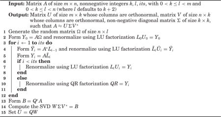
ALGORITHM 1.
Randomized SVD
|
Thus, provided that we can efficiently construct k orthonormal vectors that nearly span the range of A, we can efficiently construct an SVD that closely approximates A itself. In order to identify vectors in the range of A, we can apply A to random vectors—after all, the result of applying A to any vector is a vector in the range of A. If we apply A to k random vectors, then the results will nearly span the range of A, with extremely high probability (and the probability of capturing most of the range is even higher if we apply A to a few extra random vectors). Rigorous mathematical proofs (given by Halko et al. [2011] and by Witten and Candès [2015], for example) show that the probability of missing a substantial part of the range of A is negligible so long as the vectors to which we apply A are sufficiently random (which is so if, for example, the entries of these vectors are independent and identically distributed (i.i.d.) each drawn from a standard normal distribution). Since the results of applying A to these random vectors nearly span the range of A, applying the Gram-Schmidt process (or other methods for constructing QR decompositions) to these results yields an orthonormal basis for the approximate range of A, as desired.
This construction is particularly efficient whenever A can be applied efficiently to arbitrary vectors and is always easily parallelizable since the required matrix-vector multiplications are independent of each other. The construction of B in Equation (2) requires further matrix-vector multiplications, though there exist algorithms for the SVD of A that avoid explicitly constructing B altogether, via the application of A∗ to random vectors, identifying the range of A∗. The full process is especially efficient when both A and A∗ can be applied efficiently to arbitrary vectors and is always easily parallelizable. Further accelerations are possible when A is self-adjoint (and even more when A is nonnegative definite).
If the singular values of A decay slowly, then the accuracy of the approximation in Equation (5) may be lower than desired; the long tail of singular values that we are trying to neglect may pollute the results of applying A to random vectors. To suppress this tail of singular values relative to the singular values of interest (the leading k are those of interest), we may identify the range of A by applying AA∗ A rather than A itself—the range of AA∗ A is the same as the range of A, yet the tail of singular values of AA∗ A is lower (and decays faster) than the tail of singular values of A, relative to the singular values of interest. Similarly, we may attain even higher accuracy by applying A and A∗ in succession to each of the random vectors multiple times. The accuracy obtained thus approaches the best possible exponentially fast, irrespective of the size or even the existence of any gap in the singular values, as proven by Halko et al. [2011] (here, “exponentially fast” means that, for any positive real number ε, after at most a constant times log(1/ε) iterations the spectral-norm error of the approximation is within a small factor (1 + ε) times the optimal).
In practice, we renormalize after each application of A or A∗, as detailed in Algorithm 1, to avoid problems due to floating-point issues such as roundoff or dynamic range (overflow and underflow). The renormalized methods resemble the classical subspace or power iterations (QR or LR iterations) widely used for spectral computations, as reviewed by Golub and Van Loan [2012]. Our MATLAB codes—available at http://tygert.com/software.html (in two different versions)—provide full details, complementing the summary in Section 5 below. Other implementations of subspace iterations (which can produce accuracy beyond that needed for low-rank approximation— see, for example, Section 4) include SISVD in SVDPACK of Berry et al. [2003] and spqr_ssp in SuiteSparse of Foster and Davis [2013].
The present article focuses on calculating rank-k approximations to a matrix; a related topic is the fixed-precision problem (Algorithm 4.2 of Halko et al. [2011]), where a matrix is approximated to within precision ε (specifying ε in lieu of specifying k). For completeness, our software also includes a MATLAB implementation of the C codes by Martinsson and Voronin [2015], which provide a randomized blocked solution to the fixed-precision problem.
3. STABILIZING THE NYSTRÖM METHOD
Enhanced accuracy is available when the matrix A being approximated has special properties. For example, Algorithm 5.5 (the “Nyström¨ method”) of Halko et al. [2011] proposes the following scheme for processing a nonnegative-definite self-adjoint matrix A, given a matrix Q satisfying Equation (1), that is, A ≈ QQ∗ A, such that the columns of Q are orthonormal.
Form
| (6) |
Construct
| (7) |
Compute a triangular matrix C for the Cholesky decomposition
| (8) |
Solve for F in a system of linear equations
| (9) |
| (10) |
(However, directly computing and applying the pseudoinverse C+ would not be backward stable, so we solve for F by performing a triangular solve instead.) Compute the SVD
| (11) |
where the columns of U are orthonormal, the columns of V are also orthonormal, S is diagonal, and all entries of S are nonnegative. Set
| (12) |
Then (as demonstrated by Halko et al. [2011]) A ≈ UΣU∗, and the accuracy of this approximation should be better than that obtained using Equations (2)–(4).
Unfortunately, this procedure can be numerically unstable. Even if A is self-adjoint and nonnegative-definite, B2 constructed in Equation (7) may not be strictly positive definite (especially with roundoff errors), as required for the Cholesky decomposition in Equation (8). To guarantee numerical stability, we need only replace the triangular matrix for the Cholesky decomposition in Equation (8) from Equations (6)–(12) with the calculation of a self-adjoint square root C of B2, that is, with the calculation of a self-adjoint matrix C such that
| (13) |
The SVD of B2 provides a convenient means for computing the self-adjoint square root C.
Replacing the Cholesky factor with the self-adjoint square root is only one possibility for guaranteeing numerical stability. Our MATLAB codes instead add (and subtract) an appropriate multiple of the identity matrix to ensure strict positive definiteness for the Cholesky decomposition. This alternative is somewhat more efficient, but its implementation is more involved. The simpler approach via the self-adjoint square root should be sufficient in most circumstances.
4. MEASURING ACCURACY
For most applications of principal component analysis, the spectral norm of the discrepancy, ‖A − UΣV∗‖, where UΣV∗ is the computed approximation to A, is the most relevant measure of accuracy (a comparison to the Frobenius norm can be found in the appendix). The spectral norm ‖H‖ of a matrix H is the maximum value of |Hx|, maximized over every vector x such that |x| = 1, where Hx and |x| denote the Euclidean norms of Hx and x (the spectral norm of H is also equal to the greatest singular value of H). The spectral norm of the discrepancy between A and the optimal rank-k approximation is the (k + 1)th greatest singular value of A, usually denoted σk+1. Furthermore, the spectral norm is unitarily invariant, meaning that its value is the same with respect to any unitary transformation of the rows or any unitary transformation of the columns—that is, the value is the same with regard to any orthonormal basis of the domain and to any orthonormal basis of the range or codomain [Golub and Van Loan 2012].
If the purpose of a principal component analysis is to facilitate dimension reduction, denoising, or calibration, then the effectiveness of the approximation at reconstructing the original matrix is the relevant metric for measuring accuracy. This would favor measuring accuracy as the size of the difference between the approximation and the matrix being approximated, as in the spectral-norm discrepancy, rather than via direct assessment of the accuracy of singular values and singular vectors. The spectral norm is a uniformly continuous function of the matrix entries of the discrepancy, unlike the relative accuracy of singular values (the relative accuracy of an approximation to a singular value σ is ); continuity means that the spectral norm is stable to small perturbations of the entries [Golub and Van Loan 2012].
Fortunately, estimating the spectral norm is straightforward and reliable using the power method with a random starting vector. Theorem 4.1(a) of Kuczyński and Wozńiakowski [1992] proves that the computed estimate lies within a factor of two of the exact norm with overwhelmingly high probability, and the probability approaches 1 exponentially fast as the number of iterations increases. The guaranteed lower bound on the probability of success is independent of the structure of the spectrum; the bound is highly favorable even if there are no gaps between the singular values. Estimating the spectral-norm discrepancy via the randomized power method is simple, reliable, and highly informative.
5. ALGORITHMIC OPTIMIZATIONS
The present section describes several improvements effected in our MATLAB codes beyond the recommendations of Halko et al. [2011].
As Shabat et al. [2013] observed, computing the LU decomposition is typically more efficient than computing the QR decomposition, and both are sufficient for most stages of the randomized algorithms for low-rank approximation. Most stages just track the column space of the matrix being approximated, and the column space of the lower triangular (actually lower trapezoidal) factor in an LU decomposition is the same as the column space of the factor whose columns are orthonormal in a QR decomposition. Our MATLAB codes use LU decompositions whenever possible. For example, given some number of iterations, say, its = 4, and given an n × k random matrix Q, the core iterations in the case of a self-adjoint n × n matrix A are
for it = 1: its
 Q = A*Q;
 if (it < its)
  [Q, ~] = lu (Q);
 end
 if (it == its)
  [Q,∼,~] = qr (Q, 0);
 end
end
In all but the last of these iterations, an LU decomposition renormalizes Q after the multiplication with A. In the last iteration, a pivoted QR decomposition renormalizes Q, ensuring that the columns of the resulting Q are orthonormal. Incidentally, since the initial matrix Q was random, pivoting in the QR decomposition is not necessary; replacing the line “ [Q,∼,∼] = qr (Q, 0)” with “ [Q, ~] = qr (Q, 0)” sacrifices little in the way of numerical stability.
A little care in the implementation ensures that the same code can efficiently handle both dense and sparse matrices. For example, if c is the 1 × n vector whose entries are the means of the entries in the columns of an m × n matrix A, then the MATLAB code Q = A*Q – ones (m, 1)*(c*Q) applies the mean-centered A to Q, without ever forming all entries of the mean-centered A. Similarly, the MATLAB code Q = (Q′ *A)′ applies the adjoint of A to Q without ever forming the adjoint of A explicitly, while taking full advantage of the storage scheme for A (column-major ordering, for example).
Since the algorithms are robust to the quality of the random numbers used, we can use the fastest available pseudorandom generators, for instance, drawing from the uniform distribution over the interval [−1, 1] rather than from the normal distribution used in many theoretical analyses.
Another possible optimization is to renormalize only in the odd-numbered iterations (that is, when the variable “it” is odd in the above MATLAB code). This particular acceleration would sacrifice accuracy. However, as Rachakonda et al. [2014] observed, this strategy can halve the number of disk accesses/seeks required to process a matrix A stored on disk when A is not self-adjoint. As our MATLAB codes do not directly support out-of-core calculations, we did not incorporate this additional acceleration, preferring the slightly enhanced accuracy of our codes.
Finally, given an m × n matrix A, our implementation is optimized separately for the case m ≥ n and for the case m < n.
6. HARD PROBLEMS FOR PROPACK
PROPACK is a suite of software that can calculate low-rank approximations via remarkable, intricate Lanczos methods, developed by Larsen [2001]. Unfortunately, PROPACK can be unreliable for computing low-rank approximations. For example, using PROPACK’s principal routine, “lansvd,” under its default settings to process the diagonal matrix whose first three diagonal entries are all 1, whose 4th through 20th diagonal entries are all 0.999, and whose other entries are all 0 yields the following wildly incorrect estimates for the singular values 1, 0.999, and 0:
rank-20 approximation to a 30 × 30 matrix: 1.3718, 1.3593, 1.3386, 1.3099, 1.2733, 1.2293, 1.1780, 1.1201, 1.0560, 1.0000, 1.0000, 1.0000, 0.9990, 0.9990, 0.9990, 0.9990, 0.9990, 0.9990, 0.9990, 0.9990 (all values should be 1 or 0.999)
rank-21 (with similar results for higher rank) approximation to a 30 30 matrix: 1.7884, 1.7672, 1.7321, 1.6833, 1.6213, 1.5466, 1.4599, 1.3619, 1.2537, 1.1361, 1.0104, 1.0000, 1.0000, 1.0000, 0.9990, 0.9990, 0.9990, 0.9990, 0.9990, 0.9990, 0.9990 (this last value should be 0; all others should be 1 or 0.999)
rank-50 approximation to a 100 × 100 matrix: 1.3437, 1.3431, 1.3422, 1.3409, 1.3392, 1.3372, 1.3348, 1.3321, 1.3289, 1.3255, 1.3216, 1.3174, 1.3128, 1.3079, 1.3027, 1.2970, 1.2910, 1.2847, 1.2781, 1.2710, 1.2637, 1.2560, 1.2480, 1.2397, 1.2310, 1.2220, 1.2127, 1.2031, 1.1932, 1.1829, 1.1724, 1.1616, 1.1505, 1.1391, 1.1274, 1.1155, 1.1033, 1.0908, 1.0781, 1.0651, 1.0519, 1.0385, 1.0248, 1.0110, 1.0000, 1.0000, 1.0000, 0.9990, 0.9990, 0.9990 (the last 30 values should be 0; all others should be 1 or 0.999)
While this example was constructed specifically to be challenging for PROPACK, it demonstrates the care that must be taken when using Lanczos methods to perform low-rank approximation. Full reorthogonalization fixes this—as Rasmus Larsen, the author of PROPACK, communicated to us—but at potentially great cost in computational efficiency. Furthermore, decisions regarding reorthogonalization are nontrivial and can be challenging to implement for the nonexpert.
7. PERFORMANCE FOR DENSE MATRICES
We calculate rank-k approximations to an m × n matrix A constructed with specified singular values and singular vectors; A = UΣV∗, with U, Σ, and V constructed thus: We specify the matrix U of left singular vectors to be the result of orthonormalizing via the Gram-Schmidt process (or via an equivalent using QR decompositions) m vectors, each of length m, whose entries are i.i.d. Gaussian random variables of zero mean and unit variance. Similarly, we specify the matrix V of right singular vectors to be the result of orthonormalizing n vectors, each of length n, whose entries are i.i.d. Gaussian random variables of zero mean and unit variance. We specify to be the m×n matrix whose entries off the main diagonal are all zeros and whose diagonal entries are the singular values We consider six different distributions of singular values, testing each for two settings of m and n (namely m = n = 1000 and m = 100, n = 200). The first five distributions of singular values are
| (14) |
| (15) |
| (16) |
| (17) |
| (18) |
The spectral norm of A is 1 and the spectral norm of the difference between A and its best rank-k approximation is 10−5 for each of the four preceding examples. For the sixth example, we use for σ1, σ2, …, σmin(m,n) the absolute values of min(m, n) i.i.d. Gaussian random variables of zero mean and unit variance.
For each of the four parameter settings displayed in Figure 1 (namely, k = 3, m = n = 1000; k = 10, m = n = 1000; 1000; and k = 10, m = 100, n = 200), we plot the spectral-norm errors and runtimes for pcafast (our code), lansvd (PROPACK of Larsen [2001]), MATLAB’s built-in svds (ARPACK of Lehoucq et al. [1998]), and MATLAB’s built-in svd (LAPACK of Anderson et al. [1999]). For pcafast, we vary the oversampling parameter l that specifies the number of random vectors whose entries are i.i.d. as l = k+ 2, k+ 4, k+ 8, k+ 16, k+ 32; we leave the parameter specifying the number of iterations at the default, its = 2. For lansvd and svds, we vary the tolerance for convergence as tol = 10−8, 10−4, 1, 104, 108, capping the maximum number of iterations to be k—the minimum possible—when tol = 108. Each plotted point represents the averages over 10 randomized trials (the plots look similar, but slightly busier, without any averaging). The blue squares correspond to pcafast with l = k+ 2 (the default setting), the red diamonds correspond to pcafast with the other parameter settings, the purple triangles correspond to lansvd, the orange triangles correspond to lansvd, the orange triangles correspond to svds, and the green circles correspond to svd. Spectral-norm errors are plotted relative to σk+1, the error of the best possible rank-k approximation; whereas runtimes are plotted relative to the fastest runtime time for pcafast. As such, the points corresponding to the fastest and most accurate algorithms will be near the lower left corner of each graph. Clearly, pcafast, with the default parameters, reliably yields substantially higher performance. Please note that entirely erroneous results for lansvd were encountered when generating Figure 1, across all tolerance values, and were excluded from the figures.
Fig. 1.
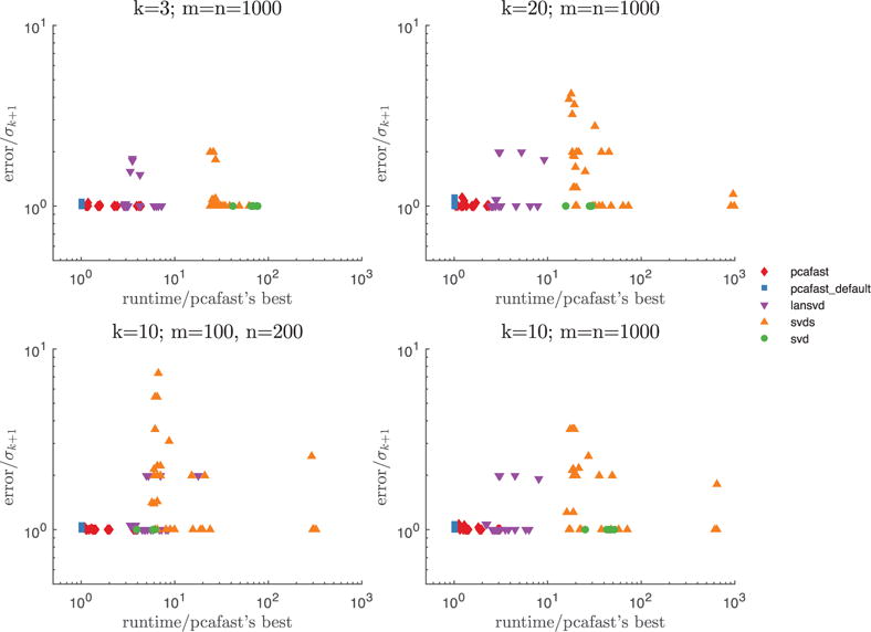
Error and runtime results for dense matrices. The only points not shown are lansvd results with relative errors exceeding 104, all of which correspond to Equation (17).
For reference, the rank of the approximation being constructed is k, and the matrix A being approximated is m × n. The plotted accuracy is the spectral norm of the difference between A and the computed rank-k approximation.
We also construct rank-4 approximations to an n × n matrix A whose entries are i.i.d. Gaussian random variables of mean and variance 1, flipping the sign of the entry in row i and column j if i · j is odd. Such a matrix has two singular values that are roughly twice as large as the largest of the others; without flipping the signs of the entries, there would be only one singular value substantially larger than the others, still producing results analogous to those reported below. For the four settings m = n = 100, 1,000, 10,000, 100,000, Figure 2 plots the spectral-norm errors and runtimes for pcafast (our code), lansvd (PROPACK of Larsen [2001]), and MATLAB’s built-in svds (ARPACK of Lehoucq et al. [1998]). For pcafast, we use 0, 2, and 4 extra power/subspace iterations (setting its = 0, 2, 4 in our MATLAB codes) and plot the case of 0 extra iterations separately, as pcafast_0its; we leave the oversampling parameter l specifying the number of random vectors whose entries are i.i.d. at the default, l = k+2. For lansvd and svds, we vary the tolerance for convergence as tol 10−2, 1, 108, capping the maximum number of iterations to be 4—the minimum possible—when = tol 108. Each plotted point represents the averages over 10 randomized trials (the plots= look similar, but somewhat busier, without this averaging). The blue squares correspond to pcafast with its = 2 (the default setting), red diamonds correspond to pcafast with its = 4, the purple triangles correspond to lansvd, the orange triangles correspond to svds, and the green circles correspond to pcafast with its 0, that is, to pcafast_0its. The plots omit svds for m = n = 100,000, since the available = memory was insufficient for running MATLAB’s built-in implementation. Clearly, pcafast is far more efficient. Some extra power/subspace iterations are necessary to yield good accuracy; except for m = n = 100,000, using only its = 2 extra power/subspace iterations yields very nearly optimal accuracy, whereas pcafast_0its (pcafast with its = 0) produces less accurate approximations.
Fig. 2.
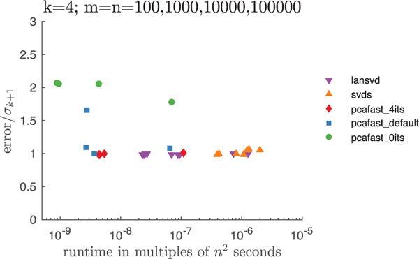
Importance of power/subspace iterations.
The computations used MATLAB 8.6.0.267246 (R2015b) on a two-processor machine, with each processor being an Intel Xeon X5650 containing six cores, where each core operated at 2.67GHz, with 12MB of L3 cache. We did not consider the MATLAB Statistics Toolbox’s own “pca,” “princomp,” and “pcacov,” as these compute all singular values and singular vectors (not only those relevant for low-rank approximation), just like MATLAB’s built-in svd (in fact, these other functions call svd).
8. PERFORMANCE FOR SPARSE MATRICES
We compute rank-k approximations to each real m × n matrix A from the University of Florida sparse matrix collection of Davis and Hu [2011] × with 200 < m < 2,000,000 and 200 < n < 2,000,000, such that the original collection provides no right-hand side for use in solving a linear system with A (matrices for use in solving a linear system tend to be so well-conditioned that forming low-rank approximations makes no sense).
For each of the six parameter settings displayed in Figure 3 (these settings are 10−3 ≤ α ≤ 10−2, as well as 10−5 ≤ α ≤ 10−4 and 10−7 ≤ α ≤ 10−6, for both k = 10 and k = 100, where α = [(number of nonzeros)/(mn)] · [k/max(m, n)]), we plot the spectral-norm errors and runtimes for pcafast (our code) and lansvd (PROPACK of Larsen [2001]). For pcafast, we vary the parameter specifying the number of iterations as its = 2, 5, 8; we leave the oversampling parameter l that specifies the number of random vectors whose entries are i.i.d. at the default, l = k + 2. For lansvd, we vary the tolerance for convergence as tol = 10−5, 1, 103. The blue squares + correspond to pcafast with parameters set at the defaults (its = 2 and l = k + 2), red diamonds correspond to pcafast with the other parameter settings, and the purple triangles correspond to lansvd. Please note that lansvd may return entirely erroneous results without warning, as indicated in Section 6.
Fig. 3.
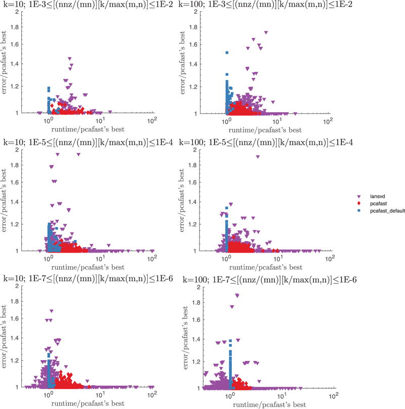
lansvd vs. pcafast applied to a total of 1,511 sparse matrices for which the values of σk+1 calculated by pcafast are not numerically zero (with “numerically zero” meaning ≤ max(m, n) ε ·‖A‖, where ε is the machine precision and A is the spectral norm of the m × n matrix A). The only points· excluded from each plot are those with relative error >2, all of which came from lansvd—the fractions of points excluded are row 1, column 1: 2.5%; row 1, column 2: 3.5%; row 2, column 1: 0.6%; row 2, column 2: 3.7%; row 3, column 1: 0.3%; row 3, column 2: 1.9%. nnz is the number of non-zero entries in the sparse matrix.
For reference, the rank of the approximation being constructed is k, and the matrix A being approximated is m × n. The plotted accuracy is the spectral norm of the difference between A and the computed rank-k approximation. The University of Florida sparse matrix collection only provides singular values for matrices with m ≤ 30,000 and n ≤ 30,000, so the accuracy of the best-possible rank-k approximation, σk+1, is not known for many matrices. As such, we plot the accuracy relative to the best pcafast accuracy.
We also use MATLAB’s built-in svds to compute rank-k approximations to each real m × n matrix A from the University of Florida collection of Davis and Hu [2011] with 200 < m < 20,000 and 200 < n < 20,000, such that the original collection provides no right-hand side for use in solving a linear system with A (matrices for use in solving a linear system tend to be so well conditioned that forming low-rank approximations makes no sense). We report this additional test since there was insufficient memory for running svds on the larger sparse matrices, so we could not include results for svds in Figure 3.
For each of the two parameter settings displayed in Figure 4 (namely, k = 10 and k = 100), we plot the spectral-norm errors and runtimes for pcafast (our code), lansvd (PROPACK of Larsen [2001]), and MATLAB’s built-in svds (ARPACK of Lehoucq et al. [1998]). For pcafast, we vary the parameter specifying the number of iterations, its = 2, 5, 8; we leave the oversampling parameter l that specifies the number of random vectors whose entries are i.i.d. at the default, l = k + 2. For lansvd, we vary the tolerance for convergence as tol = 10−5, 1, 103. For svds, we vary the tolerance as for lansvd but with 10−6 in place of 10−5 (svds requires a tighter tolerance than lansvd to attain the best accuracy). The blue squares correspond to pcafast with parameters set at the default values (its = 2 and l = k + 2), red diamonds correspond to pcafast with the other parameter settings, purple triangles correspond to lansvd, and orange triangles correspond to svds. The plotted accuracy is the spectral norm of the difference between A and the computed rank-k approximation, relative to σk+1. In Figure 4, pcafast generally exhibits higher performance than svds.
Fig. 4.
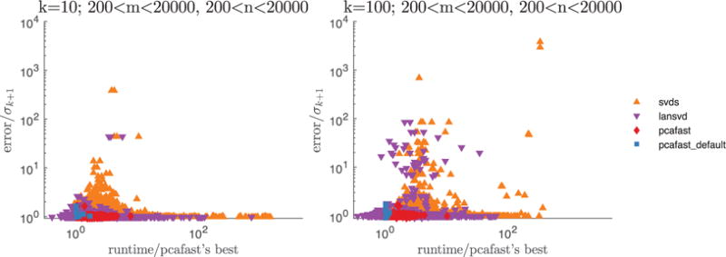
svds vs. lansvd vs. pcafast applied to a total of 958 small sparse matrices. The only points not shown correspond to 12 matrices on the left plot and 14 matrices on the right plot for which the values of σk+1 are numerically zero (with “numerically zero” meaning ≤ max(m, n) ε·‖A‖, where ε is the machine precision and ·‖A‖ is the spectral norm of the m × n matrix A).
The computations were conducted on a machine with the same specifications as in Section 7.
9. CONCLUSION
On strictly serial processors with no complicated caching (such as the processors of many decades ago), the most careful implementations of Lanczos iterations by Larsen [2001] and others could likely attain performance nearing the randomized methods’, unlike competing techniques such as the power method or the closely related nonlinear iterative partial least squares (NIPALS) of Wold [1966]. The randomized methods can attain much higher performance on parallel and distributed processors and generally are easier to use—setting their parameters properly is trivial (defaults perform well), in marked contrast to the wide variance in performance of the classical schemes with respect to inputs and parameter settings. Furthermore, despite decades of research on Lanczos methods, the theory for the randomized algorithms is more complete and provides strong guarantees of excellent accuracy, whether or not there exist any gaps between the singular values. As such, the randomized algorithms probably should be the methods of choice for computing the low-rank approximations in principal component analysis, when implemented and validated as above.
Acknowledgments
This work was supported in part by a US DoD DARPA Young Faculty Award, U.S. NIH Grant R0-1 CA158167, U.S. NIH MSTP Training Grant T32GM007205, and U.S. NIH grant 1R01HG008383-01A1.
APPENDIX: COMPARISON OF FROBENIUS- AND SPECTRAL-NORM ACCURACIES
The Frobenius norm of the difference between the approximation and the matrix being approximated is unitarily invariant as is the spectral norm, and measures the size of the discrepancy as does the spectral norm (the Frobenius norm is the square root of the sum of the squares of the absolute values of the matrix entries) [Golub and Van Loan 2012]. However, the spectral norm is generally preferable for big data subject to noise, as argued by McSherry and Achlioptas [2007]. Noise often manifests as a long tail of singular values that individually are much smaller than the leading singular values but whose total energy may approach or even exceed the leading singular values’. For example, the singular values for a signal corrupted by white noise flatten out sufficiently far out in the tail [Alliance for Telecommunications Industry Solutions Committee PRQC 2011]. The sum of the squares of the singular values corresponding to white noise or to pink noise diverges with the addition of further singular values as the dimensions of the matrix increase [Alliance for Telecommunications Industry Solutions Committee PRQC 2011]. The square root of the sum of the squares of the singular values in the tail thus overwhelms the leading singular values for big matrices subject to white or pink noise (as well as for other types of noise). Such noise can mask the contribution of the leading singular values to the Frobenius norm (that is, to the square root of the sum of squares); the “signal” has little effect on the Frobenius norm, as this norm depends almost entirely on the singular values corresponding to “noise.”
Since the Frobenius norm is the square root of the sum of the squares of all entries, the Frobenius norm throws together all the noise from all directions. Of course, noise afflicts the spectral norm, too, but only the noise in one direction at a time—noise from noisy directions does not corrupt a direction that has a high signal-to-noise ratio. The spectral norm can detect and extract a signal so long as the singular values corresponding to signal are greater than each of the singular values corresponding to noise; in contrast, the Frobenius norm can detect the signal only when the singular values corresponding to signal are greater than the square root of the sum of the squares of all singular values corresponding to noise. Whereas the individual singular values may not get substantially larger as the dimensions of the matrix increase, the sum of the squares may become troublingly large in the presence of noise. With big data, noise may overwhelm the Frobenius norm. In the words of Joel A. Tropp, Frobenius-norm accuracy may be “vacuous” in a noisy environment. The spectral norm is comparatively robust to noise.
To summarize, a long tail of singular values that correspond to noise or are otherwise unsuitable for designation as constituents of the “signal” can obscure the signal of interest in the leading singular values and singular vectors, when measuring accuracy via the Frobenius norm. Principal component analysis is most useful when retaining only the leading singular values and singular vectors, and the spectral norm is then more informative than the Frobenius norm.
Footnotes
Categories and Subject Descriptors: G.4 [Mathematical Software]: Statistical Software
Contributor Information
HUAMIN LI, Program in Applied Mathematics, 51 Prospect St., Yale University, New Haven, CT 06510.
GEORGE C. LINDERMAN, Program in Applied Mathematics, 51 Prospect St., Yale University, New Haven, CT 06510
ARTHUR SZLAM, Facebook, 8th floor, 770 Broadway, New York, NY 10003.
KELLY P. STANTON, Yale University, School of Medicine, Department of Pathology, Suite 505L, 300 George St., New Haven, CT 06520
YUVAL KLUGER, Yale University, School of Medicine, Department of Pathology, Suite 505L, 300 George St., New Haven, CT 06520.
MARK TYGERT, Facebook, 1 Facebook Way, Menlo Park, CA 94025.
References
- Alliance for Telecommunications Industry Solutions Committee PRQC. ATIS Telecom Glossary, American National Standard T1.523. Alliance for Telecommunications Industry Solutions (ATIS), American National Standards Institute (ANSI); Washington, DC: 2011. [Google Scholar]
- Anderson Edward, Bai Zhaojun, Bischof Christian, Blackford Laura Susan, Demmel James, Dongarra Jack, Du Croz Jeremy, Greenbaum Anne, Hammarling Sven, McKenney Alan, Sorensen Daniel. LAPACK User’s Guide. SIAM; Philadelphia, PA: 1999. [Google Scholar]
- Avron Haim, Bekas Costas, Boutsidis Christos, Clarkson Kenneth, Kambadur Prabhanjan, Kollias Giorgos, Mahoney Michael, Ipsen Ilse, Ineichen Yves, Sindhwani Vikas, Woodruff David. Lib-Skylark: Sketching-Based Matrix Computations for Machine Learning. IBM Research, in collaboration with Bloomberg Labs, NCSU, Stanford, UC Berkeley, and Yahoo Labs; 2014. Retrieved from http://xdata-skylark.github.io/libskylark. [Google Scholar]
- Berry Michael, Mezher Dany, Philippe Bernard, Sameh Ahmed. Research report RR-4694. INRIA; 2003. Parallel computation of the singular value decomposition. [Google Scholar]
- Davis Timothy A, Hu Yifan. The university of Florida sparse matrix collection. ACM Trans Math Softw. 2011;38(1):1. 2011. 1–1:25. [Google Scholar]
- Foster Leslie V, Davis Timothy A. Algorithm 933: Reliable calculation of numerical rank, null space bases, pseudoinverse solutions, and basic solutions using SuiteSparseQR. ACM Trans Math Softw. 2013 Sep;40(1):1–23. 2013. http://dx.doi.org/10.1145/2513109.2513116. [Google Scholar]
- Golub Gene, Van Loan Charles. Matrix Computations. 4th. Johns Hopkins University Press; 2012. [Google Scholar]
- Halko Nathan, Martinsson Per-Gunnar, Tropp Joel. Finding structure with randomness: Probabilistic algorithms for constructing approximate matrix decompositions. SIAM Rev. 2011;53(2):217–288. 2011. [Google Scholar]
- Kuczyński Jacek, Woźniakowski Henryk. Estimating the largest eigenvalue by the power and Lanczos algorithms with a random start. SIAM J Matrix Anal Appl. 1992;13(4):1094–1122. 1992. [Google Scholar]
- Larsen Rasmus. Combining implicit restart and partial reorthogonalization in Lanczos bidiagonalization. Presentation at UC Berkeley, sponsored by Stanford’s Scientific Computing and Computational Mathematics (succeeded by the Institute for Computational and Mathematical Engineering) 2001 Retrieved from http://sun.stanford.edu/∼rmunk/PROPACK/talk.rev3.pdf.
- Lehoucq Richard, Sorensen Daniel, Yang Chao. ARPACK User’s Guide: Solution of Large-Scale Eigenvalue Problems with Implicitly Restarted Arnoldi Methods. SIAM; Philadelphia, PA: 1998. [Google Scholar]
- Martinsson Per-Gunnar, Voronin Sergey. A randomized blocked algorithm for efficiently computing rank-revealing factorizations of matrices. 2015:1–12. [Google Scholar]
- McSherry Frank, Achlioptas Dimitris. Fast computation of low-rank matrix approximations. J ACM. 2007 Apr;54(2):1–19. 2007. [Google Scholar]
- Rachakonda Srinivas, Silva Rogers F, Liu Jingyu, Calhoun Vince. Memory-efficient PCA approaches for large-group ICA (2014) fMRI Toolbox, Medical Image Analysis Laboratory, University of New Mexico; 2014. [Google Scholar]
- Shabat Gil, Shmueli Yaniv, Averbuch Amir. Randomized LU Decomposition. Technical Report 1310.7202. 2013:arXiv. [Google Scholar]
- Witten Rafi, Candès Emmanuel. Randomized algorithms for low-rank matrix factorizations: Sharp performance bounds. Algorithmica. 2015 May;72(1):264–281. 2015. [Google Scholar]
- Wold Herman. Estimation of principal components and related models by iterative least squares. In: Krishnaiaah Parachuri R., editor. Multivariate Analysis. Academic Press; 1966. pp. 391–420. [Google Scholar]
- Woodruff David. Sketching as a Tool for Numerical Linear Algebra. Vol. 10. Foundations and Trends in Theoretical Computer Science; 2014. Now Publishers. [Google Scholar]