A predictive probability design for phase II cancer clinical trials

Abstract

Background

Two- or three-stage designs are commonly used in phase II cancer clinical trials. These designs possess good frequentist properties and allow early termination of the trial when the interim data indicate that the experimental regimen is inefficacious. The rigid study design, however, can be difficult to follow exactly because the response has to be evaluated at pre-specified fixed number of patients.

Purpose

Our goal is to develop an efficient and flexible design that possesses desirable statistical properties.

Method

A flexible design based on Bayesian predictive probability and the minimax criterion is constructed. A three-dimensional search algorithm is implemented to determine the design parameters.

Results

The new design controls type I and type II error rates, and allows continuous monitoring of the trial outcome. Consequently, under the null hypothesis when the experimental treatment is not efficacious, the design is more efficient in stopping the trial earlier, which results in a smaller expected sample size. Exact computation and simulation studies demonstrate that the predictive probability design possesses good operating characteristics.

Limitations

The predictive probability design is more computationally intensive than two- or three-stage designs. Similar to all designs with early stopping due to futility, the resulting estimate of treatment efficacy may be biased.

Conclusions

The predictive probability design is efficient and remains robust in controlling type I and type II error rates when the trial conduct deviates from the original design. It is more adaptable than traditional multi-stage designs in evaluating the study outcome, hence, it is easier to implement. S-PLUS/R programs are provided to assist the study design.

1. INTRODUCTION

Phase II studies play a pivotal role in drug development. The main purpose for phase II clinical trials is to determine whether a new treatment demonstrates sufficient efficacy to warrant further investigation. It helps to screen out inefficacious agents and avoid sending them to large phase III trials. [1,2] A commonly used primary endpoint in phase II cancer clinical trials is the clinical response to a treatment, which is a binary endpoint defined as the patient achieving complete or partial response within a pre-defined treatment course. In the early phase II development of new drugs, most trials are open label, single-arm studies, while late phase II trials tend to be multi-arm, randomized studies. Overviews of statistical methods for phase II trials can be found in the work of Thall and Simon [3], Kramar et al. [4], Mariani and Marubini [5], and Lee and Feng.[6]

In this paper, we focus on the one arm phase II trials with binary endpoints. Multi-stage designs are often implemented in such settings to increase the study efficiency by allowing early termination if the treatment is deemed inefficacious. The first phase II design proposed for cancer research is a two-stage procedure by Gehan. [7] With that design, if no responses are observed in the first stage, the new treatment is abandoned. Otherwise, additional patients are enrolled in the second stage to provide a better estimation of the response rate. The commonly used Simon’s designs [8] are also two-stage designs. Simon’s designs allow early stopping due to futility, i.e., when lack of efficacy is observed. If the experimental treatment works well, more patients aretreated in the second stage, which also allows better estimation of the response rate and toxicity of the new treatment, before launching a phase III trial. Under the null hypothesis, the optimal two-stage design minimizes the expected sample size, while the minimax design minimizes the maximum sample size. Both designs are subject to the constraints of type I and type II error rates. Many other multi-stage designs with different objectives and optimization criteria can be found in the literature. [9–12] Jung et al. devised a graphical method for searching all design parameters to attain certain admissible two-stage designs with good design characteristics.[13] They later generalized the method and identified a family of admissible designs using a Bayesian decision-theoretic criterion.[14]

Multi-stage designs possess better statistical properties than single-stage designs by utilizing the information gained in the interim data. Furthermore, three-stage designs are generally more efficient than two-stage designs because the additional interim look at the data allows for earlier decision to stop the trial if convincing evidence to support the null or alternative hypothesis is found. These designs, however, are more difficult to conduct because of the rigid requirement of examining the outcome at the specified sample size in each fixed stage. The strict sample size guideline in each stage is particularly difficult to adhere to in multi-center trials due to the complexity of coordinating patient accrual and follow-up across multiple sites. Temporarily halting the study accrual can also stall the momentum of the trial and lower the enthusiasm for investigators to participate in the trial. In addition, when the actual conduct deviates from the original design, the stopping boundaries are left undefined and the planned statistical properties no longer hold. Many authors have recognized this problem and have offered solutions. Green and Dahlberg [15] examined the performance of planned versus attained designs and gave an empirical solution by adapting the stopping rules to achieve desirable statistical properties when the actual sample size deviates from the planned one. Herndon proposed a hybrid design by blending the one-stage and two-stage designs, which allows uninterrupted accrual between the stages.[16] Chen and Ng [17] gave a collection of two-stage designs with a range of sample sizes in the first and second stages to construct optimal flexible designs.

Another limitation of the fixed design is that even after an extra long series of failures is observed, there is no formal mechanism to stop the trial before the predetermined sample size is reached. Furthermore, investigators often need to decide whether to continue or to terminate a trial at certain interim points, not always at the time points initially planned, due to slow accrual or other practical considerations.[18] This lack of design flexibility exposes a fundamental limitation of all frequentist-based methods because statistical inference is made by computing the probability of observing certain data conditioned on a particular design and the sampling plan. When there is a disparity between the proposed design and the actual trial conduct, which is more a norm than an exception in clinical trials, adjustments must be made in all statistical inferences. All these reasons support the need for more flexible designs.

Bayesian methods, on the other hand, offer a different approach for designing and monitoring clinical trials by computing the probability of parameters given data. Based on the likelihood principle, all information pertinent to the parameters is contained in the data and is not constrained by the design. Bayesian methods are particular appealing in clinical trial design because, inherently, they allow for flexibility in trial conduct and impart the ability to examine interim data, update the posterior probability of parameters, and make sensible decisions accordingly. Bayesian methods can also incorporate relevant information, both internal and external to the trial, for decision making.[19,20] Several Bayesian phase II designs have been proposed in the literature. Sylvester proposed a decision theoretical approach by minimizing the expected loss to determine an optimal Bayesian design.[21] Thall and Simon developed a design withcontinuous monitoring until achieving a high posterior probability that either a drug is promising or not promising, or until reaching the maximum sample size.[22,23] Also based on the posterior probability, Heitjan [24] advocated the use of “persuasion probability” as a consistent criterion for determining whether the drug is promising or not. Tan and Machin [25] constructed Bayesian two-stage designs, which mimic the frequentist alternatives, by calibrating design parameters based on the posterior probability approach. Similar approaches based on informative priors or mixtures of informative priors have also been reported.[26,27]

Applying the concept of predictive probability, we take the proper Bayesian approach in the sense that we apply the full likelihood approach, but without specifying the loss function, as in the decision theoretical approach. Hence, we do not compute the Bayes risk.[28] One advantage of the predictive probability approach is that it closely mimics the clinical decision making process. Predictive probability is obtained by calculating the probability of a positive conclusion (rejecting the null hypothesis) should the trial be conducted to the maximum planned sample size given the interim observed data. In this framework, the chance that the trial will show a conclusive result at the end of the study, given the current information, is evaluated. Then, the decision to continue or to stop the trial can be made according to the strength of the predictive probability. Several adaptations of predictive probability approaches for interim monitoring of clinical trials have been discussed. [29–31,33–35,42] Notably, Choi et al. [29] calculated predictive probability in making an early decision in a large sample two-arm trial where the outcome is the proportion of successes, using normal approximation under a large sample assumption. Spiegelhalter et al. [31] suggested that the predictive power, derived by averaging the conditional power based on current data over the current belief about the unknown parameters, should be used to detect significant differences between treatments. As for trial design, Herson [36] first proposed the predictive probability approach for designing phase II clinical trials with dichotomous outcomes. The proposed maximum sample size and critical region are originated from a frequentist one-stage design. The choice of the cutoff values for the predictive probability is somewhat arbitrary and does not guarantee the type I and type II error rates.

Under the predictive probability framework, our approach searches for the design parameters within the given constraints such that both the size and power of the test can be guaranteed. In section 2, we give an overview of Simon’s two-stage design and define the proposed predictive probability approach in a Bayesian setting. Exact computation and a searching procedure have been developed to facilitate the predictive probability design. In Section 3, we investigate the property of the predictive probability approach and compare its performance with Simon’s two-stage design through several examples. In Section 4, we describe the simulation studies for evaluating the robustness of the design when trial conduct deviates from the originally proposed design and when the trial is stopped prematurely. The estimation bias and the comparison between the predictive probability versus the posterior probability approaches are also given. We provide a discussion in Section 5.

2. METHODS FOR SIMON’S TWO-STAGE DESIGN AND PREDICTIVE PROBABILITY DESIGN

Under the hypothesis testing framework, a phase IIA clinical trial is designed to test

$$H_0:p\le p_0$$

$$H_1:p\ge p_1$$

where p₀ represents a pre-specified response rate of the standard treatment and p₁ represents a target response rate of a new treatment. A study is designed such that

$$P(\mathit{Accept}\mathit{New}\mathit{Treatment}|H_0)\le \alpha$$

$$\text{and}P(\mathit{Reject}\mathit{New}\mathit{Treatment}|H_1)\le \beta$$

where α and β are type I and type II error rates, respectively. Given p₀, p₁, the maximum number of patients, number of stages, cohort size at each stage, acceptance region and rejection region at each stage, the type I and type II error rates, the probability of early termination (PET) of the trial and the expected sample size (E(N)) under H₀ can be calculated by applying the recursive formulas of Schultz et al. [37] A desirable design is one with operating characteristics that satisfy the constraints of the type I and type II error rates, with a high probability of early termination and a small expected sample size under H₀. Note that we define the acceptance region as the outcome space leading to the acceptance of the new treatment (i.e., reject the null hypothesis) and, the rejection region as the outcome space leading to the rejection of the agent (i.e., fail to reject the null hypothesis).

2.1. Simon’s two-stage designs

The algorithm for implementing Simon’s two-stage designs is as follows:

• Stage I: Enroll n₁ patients. Stop the trial and reject the new treatment (stop for futility) if the number of observed responses, x₁, is r₁ or less. Otherwise, continue to stage II.

• Stage II: Enroll (N_max − n₁) patients to reach a total of N_max patients. Reject the new treatment if the number of responses is r or less. Otherwise, consider that the new treatment warrants further development.

Based on these decision rules, PET and E(N) under H₀ can be calculated:

PET(p₀) = Prob(Early Termination | H₀) = Prob(X₁ ≤ r₁|H₀), where X₁ is the number of responses in n₁(n₁ < N_max) patients from the first stage, and X₁ follows a binomial distribution with X₁ ~ binomial(n₁, p₀),

$$E(N|p_0)=n_1+[1-\mathit{PET}(p_0)]\times (N_{\mathit{max}}-n_1)$$

Among all designs that satisfy the constraint of the type I and type II error rates, Simon’s optimal two-stage design is obtained when E(N | p₀) is the smallest. On the other hand, the minimax design is defined when the maximum sample size is the smallest.

2.2. Predictive probability approach in a Bayesian setting

In the Bayesian approach, we assume that the prior distribution of the response rate π(p) follows a beta distribution, beta(a₀, b₀). It represents the investigator’s previous knowledge or belief of the efficacy of the new regimen. The quantity a₀/(a₀ + b₀) reflects the prior mean while size of a₀ + b₀ indicates how informative the prior is. The quantities a₀ and b₀ can be considered as the number of response and the number of non-responses, respectively. Thus, a₀ + b₀ can be considered as a measure of the amount of information contained in the prior. The larger the value of a₀ + b₀, the more informative the prior and the stronger the belief it contains. We set a maximum accrual of patients to N_max. We assume the number of responses in the current n (n ≤ N_max) patients, X, follows a binomial distribution, binomial(n, p), and the likelihood function for the observed data x is

$$L_x(p)\propto p^x\times {(1-p)}^{n-x}.$$

Consequently, the posterior distribution of the response rate follows a beta distribution

$$P|x\sim \mathit{beta}(a_0+x,b_0+n-x).$$

Thus, the number of responses in the potential m = N_max − n future patients, Y, follows a beta-binomial distribution, beta-binomial(m, a₀ + x, b₀ + n − x).

When Y = i, we denote the posterior probability of P as

$$f(p|X=x,Y=i),\text{where}P|X=x,Y=i\sim \mathit{beta}(a_0+x+i,b_0+N_{\mathit{max}}-x-i).$$

From here on, the observed response X = x will be abbreviated as x. To calculate the predictive probability, we further define

$$B_i=\mathit{Prob}(P>p_0|x,Y=i),$$

where P follows a beta distribution. B_i measures the probability that the response rate is larger than p₀ given x responses in n patients in the current data and i responses in m future patients. Comparing B_i to a threshold value θ_T yields an indieator I_i for considering that the treatment is efficacious at the end of the trial given the current data and the potential outcome of Y = i (see Table 1A for a schematic representation).

Table 1.

Bayesian predictive probability approach: A schema and an example.

A. Schema
Y=i	Prob(Y=i | x)	Bi=Prob(P>p0 | x, Y=i)	Ii(Bi> θT)
0	Prob(Y=0 | x)	B0=Prob(P>p0 | p, f(p|x, Y=0))	0
1	Prob(Y=0 | x)	B1=Prob(P>p0 | p, f(p|x, Y=1))	0
…	…	…	…
m-1	Prob(Y=m-1| x)	Bm-1 =Prob(P>p0 | p, f(p|x, Y=m-1))	1
m	Prob(Y=m | x)	Bm =Prob(P>p0 | p, f(p|x, Y=m))	1

B. Example: Nmax = 40, x = 16, n = 23, prior distribution of P ~ beta(0.6, 0.4)
Y=i	Prob(Y=i | x)	Bi=Prob(P>60% | x, Y=i)	Ii(Bi>0.90)
0	0.0000	0.0059	0
1	0.0000	0.0138	0
2	0.0001	0.0296	0
3	0.0006	0.0581	0
4	0.0021	0.1049	0
5	0.0058	0.1743	0
6	0.0135	0.2679	0
7	0.0276	0.3822	0
8	0.0497	0.5085	0
9	0.0794	0.6349	0
10	0.1129	0.7489	0
11	0.1426	0.8415	0
12	0.1587	0.9089	1
13	0.1532	0.9528	1
14	0.1246	0.9781	1
15	0.0811	0.9910	1
16	0.0381	0.9968	1
17	0.0099	0.9990	1

We define

$$\begin{gathered} \mathit{Predictive}\mathit{Probability}(PP) \\ ={\displaystyle \sum _{i=0}^m\{\mathit{Prob}(Y=i|x)\times I(\mathit{Prob}(P>p_0|x,Y=i)>{\theta }_T)\}} \\ ={\displaystyle \sum _{i=0}^m\{\mathit{Prob}(Y=i|x)\times I(B_i>{\theta }_T)\}={\displaystyle \sum _{i=0}^m\{\mathit{Prob}(Y=i|x)\times I_i\}}} \end{gathered}$$

where Prob(Y = i | x) is the probability of observing i responses in m patients given current data x where Y follows a beta-binomial distribution. The weighted sum of indicator I_i over Y yields the predictive probability (PP) of concluding a positive result by the end of the trial based on the cumulative information in the current stage. A high PP means that the treatment is likely to be efficacious by the end of the study, given the current data, whereas a low PP suggests that the treatment may not have sufficient activity. Therefore, PP can be used to determine whether the trial should be stopped early due to efficacy/futility or continued because the current data are not yet conclusive. The decision rules can be constructed as follows:

• If PP < θ_L, then stop the trial and reject the alternative hypothesis;

• If PP > θ_U, then stop the trial and reject the null hypothesis;

• Otherwise continue to the next stage until reaching N_max patients.

Typically, we choose θ_L as a small positive number and θ_U as a large positive constant, both between 0 and 1 (inclusive). PP < θ_L indicates that it is unlikely the response rate will be larger than p₀ at the end of the trial given the current information. When this happens, we may as well stop the trial and reject the alternative hypothesis at that point. On the other hand, when PP > θ_U, the current data suggest that, if the same trend continues, we will have a high probability to conclude that the treatment is efficacious at the end of the study. This result, then, provides evidence to stop the trial early due to efficacy. By choosing θ_L > 0 and θ_U < 1.0, the trial can terminate early due to either futility or efficacy. For phase IIA trials, we prefer to choose θ_L > 0 and θ_U = 1.0 to allow early stopping due to futility, but not due to efficacy.

For example (see Table 1B), in a phase II trial, an investigator plans to enroll a maximum of N_max = 40 patients into the study. At a given time, x = 16 responses are observed in n = 23 patients. What is P(response rate > 60%)? Assuming a prior distribution of response rate (p) as beta(0.6, 0.4) and with the number of responses in future m = 17 patients, Y follows a beta-binomial distribution, beta-binomial(17, 16.6, 7.4). At each possible value of Y = i, the posterior probability of P follows a beta distribution, P|x, Y = i ~ beta(16.6 + i, 24.4 − i). In this example, we set θ_T = 0.90. As it can be seen, when Y is in the range from 0 to 11, the resulting P(response rate > 60%) ranges from 0.0059 to 0.8415. Hence, we will conclude H₀ for Y ≤ 11,. On the other hand, when Y goes from 12 to 17, the resulting P(response rate > 60%) ranges from 0.9089 to 0.9990. Therefore,, we will conclude H₁ for Y ≥ 12. The predictive probability is then the weighted average (weighted by the probability of the realization of each Y) of the indicator of a positive trial should the current trend continue and the trial be conducted until the end of the study. The calculation yields PP = 0.5656. If we choose θ_L = 0.10, the trial will not be stopped because PP is greater than θ_L

2.3. Designing a trial using the PP approach: Search N_max, θ_L, θ_T and θ_U for the PP design to satisfy the constraints of the type I and type II error rates

Given p₀, p₁, the prior distribution of response rate π(p) and the cohort size for interim monitoring, we search the design parameters, including the maximum sample size N_maxi θ_L, θ_T and θ_U, to yield a design satisfying the type I and type II error rates constraints simultaneously. As mentioned earlier, we choose θ_U = 1.0 because if the treatment is working, there is little reason to stop the trial early – enrolling more patients to the active treatment is good. Treating more patients until the maximum sample size is reached (usually, less than 100) can also increase the precision in estimating the response rate. Given N_max, the question is, “Are there values of θ_L and θ_T that yield desirable design properties”? By searching over all possible values of θ_L and θ_T, our goal is to identify the combinations of θ_L and θ_T to yield the desirable power within the constraint of the specified type I error rates. There may exist ranges of θ_L and θ_T that satisfy the constraints. By varying N_max from small to large, the design with the smallest N_max that controls both type I and type II error rates at the nominal level is the one we choose. This idea is similar to finding the minimax design, i.e., minimizing the maximum sample size.

The framework of this PP method allows the investigator to monitor the trial continuously or by any cohort size. We choose to start computing PP and making interim decisions after the first 10 patients have been treated and evaluated for their response status. Although the choice of treating a minimum of 10 patients is somewhat arbitrary, a minimum number of patients is required to provide sufficient information in order to obtain a good estimate of the treatment efficacy and avoid making premature decisions based on spurious results from a small number of patients. After 10 patients, we calculate PP continuously (i.e., with cohort size of 1) to monitor the treatment efficacy. If PP is low, the data indicate that the treatment may not be efficacious. A sufficiently low PP (e.g., PP < θ_L) suggests that the trial could be stopped early due to lack of efficacy. Note that PP can be computed for any cohort size and at any interim time. A trial can be stopped anytime due to excessive toxicity, however.

3. COMPARISON BETWEEN PREDICTIVE PROBABILITY APPROACH AND SIMON’S TWO-STAGE DESIGN

The comparison between the PP design and Simon’s two-stage design is performed by examining the design’s operating characteristics, such as the type I error rate, power, PET(p₀) and E(N | p₀). The concept of designing trials using the PP approach is illustrated in the following examples.

3.1. Example 1: A lung cancer trial

The primary objective of this study is to assess the efficacy of a combination therapy as front-line treatment in patients with advanced non-small cell lung cancer. The study involves the combination of a vascular endothelial growth factor antibody plus an epidermal growth factor receptor tyrosin kinase inhibitor. The primary endpoint is the clinical response rate (i.e., rate of complete response and partial response combined) to the new regimen. The current standard treatment yields a response rate of approximately 20% (p₀). The target response rate of the new regimen is 40% (p₁). With the constraint of both type I and type II error rates ≤0.1, Simon’s optimal two-stage design yields n₁=17, r₁=3, N_max=37, r=10, PET(p₀) =0.55 and E(N | p₀)=26.02 with α=0.095 and, β=0.097. The corresponding minimax design yields n₁=19, r₁=3, N_max=36, r=10, PET(p₀) =0.46 and E(N | p₀)=28.26 with α=0.086 and β=0.098.

Taking the PP approach, we assume that the response rate P has a prior distribution of beta(0.2, 0.8). The trial is monitored continuously after evaluating the responses of the first 10 patients. For each N_max between 25 and 50, we search the θ_L and θ_T space to generate designs that have both type I and type II error rates under 0.10. Table 2 lists some of the results in the order of the maximum sample size, N_max. Among all the designs, the design with N_max = 36 (boldfaced type) is the design with the smallest N_max that has both type I and type II error rates controlled under 0.1.

Table 2.

Operating characteristics of Simon’s two-stage designs and the PP design with type I and type II error rates ≤ 0.10, prior for p = beta(0.2,0.8), p₀=0.2, p₁=0.4

Simon’s Minimax/Optimal 2-Satge
	r1/n1	r/Nmax	PET(p0)	E(N| p0)	α	β
Minimax	3/19	10/36	0.46	28.26	0.086	0.098
Optimal	3/17	10/37	0.55	26.02	0.095	0.097

Predictive Probability
θL	θT	r/Nmax	PET(p0)	E(N| p0)	α	β
0.001	[0.852,0.922]*	10/36	0.86	27.67	0.088	0.094
0.011	[0.830,0.908]	10/37	0.85	25.13	0.099	0.084
0.001	[0.876,0.935]	11/39	0.88	29.24	0.073	0.092
0.001	[0.857,0.923]	11/40	0.86	30.23	0.086	0.075
0.003	[0.837,0.910]	11/41	0.85	30.27	0.100	0.062
0.043	[0.816,0.895]	11/42	0.86	23.56	0.099	0.083
0.001	[0.880,0.935]	12/43	0.88	32.13	0.072	0.074
0.001	[0.862,0.924]	12/44	0.87	33.71	0.085	0.059
0.001	[0.844,0.912]	12/45	0.85	34.69	0.098	0.048
0.032	[0.824,0.898]	12/46	0.86	26.22	0.098	0.068
0.001	[0.884,0.936]	13/47	0.89	35.25	0.071	0.058
0.001	[0.868,0.925]	13/48	0.87	36.43	0.083	0.047
0.001	[0.850,0.914]	13/49	0.86	37.86	0.095	0.038
0.020	[0.832,0.901]	13/50	0.86	30.60	0.100	0.046

^*The numbers within the bracket indicate a closed interval with both endpoints included.

Based on this setting, θ_L and θ_T are determined to be 0.001 and [0.852, 0.922], respectively. The corresponding rejection region (in number of response/n) is 0/10, 1/17, 2/21, 3/24, 4/27, 5/29, 6/31, 7/33, 8/34, 9/35 and 10/36. The trial will be stopped and the treatment is considered ineffective when the number of responses first falls into the rejection region. Based on these boundaries, if the true response rate is 20%, the probability of accepting the treatment is 0.088. On the other hand, if the true response rate is 40%, the probability of accepting the treatment is 0.906. The probability of stopping the trial early is 0.86 and the expected sample size is 27.67 when the true response rate is 20%. Compared to Simon’s minimax two-stage design, the trial is monitored more frequently in the PP design, which also has a larger probability of early termination and a smaller expected sample size in the null case. Both designs have the same maximum sample size with controlled type I and type II error rates.

3.2. Example 2: A tongue cancer trial

The primary objective of a second study is to assess the efficacy of induction chemotherapy (with paclitaxel, ifosfamide, and carboplatin) followed by radiation in treating young patients with prior untreated squamous cell carcinoma of the tongue. Previous results show that radiation alone gives a response rate of 60% (p₀). With induction chemotherapy plus radiation, the target response rate is set at 80% (p₁). Under the constraint of a type I error rate ≤ 0.05 and a type II error rate ≤ 0.20, Simon’s optimal two-stage design yields n₁=11, r₁=7, N_max=43, r=30, PET(p₀)=0.70, and E(N | p₀)=20.48 with α=0.049, β=0.198. The corresponding minimax design yields n₁=13, r₁=8, N_max=35, r=25, PET(p₀) =0.65 and E(N | p₀)=20.77 with α=0.050 and β=0.192.

Taking the PP approach, we search the design parameters with a maximum number of patients ranging between 25 and 44, assuming the prior distribution of the response rate as beta(0.6, 0.4), and using continuous monitoring after the first 10 patients are evaluated. Table 3 lists the resulting designs. We find that the design with the smallest N_max that has desirable type I and II error rates is the one with N_max = 35 (shown in boldface type in Table 3), where θ_L and θ_T are in the ranges of [0.075, 0.079] and [0.924, 0.963], respectively. In this design, if the true response rate is 60%, the probability of accepting the treatment is 0.050, the probability of early termination of the trial is 0.94 and the expected sample size is 16.87. On the other hand, if the true response rate is 80%, the probability of accepting the treatment is 0.815. Again, compared to Simon’s designs, the trial is monitored more frequently applying the PP approach and has a higher probability of early stopping with a smaller expected sample size, if the regimen is not efficacious. In this example, the maximum number of patients under the PP approach is also the same as that under Simon’s minimax two-stage design.

Table 3.

Operating characteristics of Simon’s two-stage designs and the PP design with type I error rate ≤ 0.05 and type II error rate≤0.20, prior for p = beta(0.6,0.4), p₀=0.6, p₁=0.8

Simon’s Minimax/Optimal 2-Satge
	r1/n1	r/Nmax	PET(p0)	E(N| p0)	α	β
Minimax	8/13	25/35	0.65	20.77	0.050	0.192
Optimal	7/11	30/43	0.70	20.48	0.049	0.198

Predictive Probability
θL	θT	r/Nmax	PET(p0)	E(N| p0)	α	β
[0.075,0.079]	[0.924,0.963]*	25/35	0.94	16.87	0.050	0.1855
0.001	[0.940,0.972]	26/36	0.94	23.16	0.045	0.168
0.001	[0.953,0.978]	27/37	0.96	23.05	0.035	0.191
[0.061,0.067]	[0.925,0.963]	27/38	0.94	18.20	0.050	0.158
0.001	[0.941,0.971]	28/39	0.94	25.12	0.045	0.141
0.001	[0.953,0.978]	29/40	0.96	24.87	0.035	0.161
0.051	[0.927,0.962]	29/41	0.94	19.57	0.0500	0.135
0.001	[0.942,0.971]	30/42	0.94	27.28	0.045	0.119
0.001	[0.954,0.977]	31/43	0.96	26.88	0.035	0.136
0.051	[0.929,0.962]	31/44	0.94	21.40	0.050	0.111

^*The numbers within the bracket indicate a closed interval with both endpoints included.

3.3. More examples

Operating characteristics of more examples using Simon’s minimax and optimal two-stage designs, and the PP design are shown in Table 4, with p₀=0.1 to 0.7 % 0.1 intervals, p₁ − p₀ = 0.2, type I and type II error rates of 0.10, and continuous monitoring after the first 10 evaluable patients in the PP design. While the type I and type II error rates are controlled in both PP and Simon’s two-stage designs, the probability of stopping the trial early is always larger in the PP design. In addition, we find that the PP design has a smaller expected sample size under the null hypothesis in all cases except when p₀ = 0.1 and p₁ = 0.3. Compared to multi-stage designs, PP designs are also more flexible to conduct and have more robust design properties when the trial conduct does not follow the plan exactly. This topic is described in greater detail in the next section.

Table 4.

Operating characteristics of additional examples using Simon’s two-stage designs and the PP design with type I and type II error rates of 0.10

	Simon’s Minimax/Optimal Two Stage Design+						Predictive Probability Design
P0/p1	r1/n1	r/Nmax	PET(p0)	E(N| p0)	α	β	θL	θT	r/Nmax	PET(p0)	E(N| p0)	α	β
0.1/0.3	1/16	4/25	0.52	20.37	0.095	0.097	0.001	[0.782,0.911]*	4/25	0.79	19.99	0.096	0.095
	1/12	5/35	0.66	19.84	0.098	0.099	0.001	[0.855,0.942]	5/29	0.86	21.98	0.062	0.099
							0.001	[0.838,0.933]	5/30	0.85	23.25	0.072	0.081
							0.001	[0.821,0.924]	5/31	0.83	23.94	0.082	0.068
							0.001	[0.804,0.913]	5/32	0.81	25.42	0.093	0.054
							0.003	[0.786,0.902]	5/33	0.81	23.50	0.100	0.056
							[0.037,0.046]	[0.767,0.890]	5/34	0.84	19.96	0.099	0.069
							0.001	[0.879,0.949]	6/35	0.89	26.01	0.054	0.070
							0.001	[0.866,0.942]	6/36	0.87	26.75	0.061	0.059
							0.001	[0.852,0.934]	6/37	0.86	28.16	0.070	0.048
							0.001	[0.838,0.926]	6/38	0.85	29.14	0.078	0.040
0.2/0.4	3/19	10/36	0.46	28.26	0.086	0.098	0.001	[0.852,0.922]	10/36	0.86	27.67	0.088	0.094
	3/17	10/37	0.55	26.02	0.095	0.097	0.011	[0.830,0.908]	10/37	0.85	25.13	0.100	0.084
							0.001	[0.876,0.935]	11/39	0.88	29.24	0.073	0.092
							0.001	[0.857,0.923]	11/40	0.86	30.23	0.086	0.075
							0.003	[0.837,0.910]	11/41	0.85	30.27	0.100	0.062
							0.043	[0.816,0.895]	11/42	0.86	23.56	0.099	0.083
0.3/0.5	7/28	15/39	0.37	34.99	0.094	0.100	0.001	[0.859,0.918]	16/42	0.86	32.47	0.096	0.083
	7/22	17/46	0.67	29.89	0.097	0.095	0.001	[0.881,0.932]	17/44	0.88	33.50	0.081	0.088
							0.001	[0.858,0.916]	17/45	0.86	34.84	0.098	0.069
							0.048	[0.834,0.899]	17/46	0.87	25.11	0.099	0.092
							0.001	[0.880,0.929]	18/47	0.88	35.70	0.083	0.073
							0.001	[0.858,0.914]	18/48	0.86	37.33	0.100	0.056
0.4/0.6	11/28	20/41	0.55	33.84	0.095	0.099	0.001	[0.868,0.923]	20/41	0.87	31.07	0.096	0.098
	7/18	22/46	0.56	30.22	0.095	0.100	0.001	[0.875,0.927]	21/43	0.88	32.12	0.091	0.093
							0.001	[0.882,0.930]	22/45	0.89	33.65	0.086	0.087
							[0.024,0.025]	[0.854,0.911]	22/46	0.87	27.33	0.100	0.084
							0.001	[0.889,0.934]	23/47	0.89	35.00	0.082	0.082
							[0.010,0.011]	[0.862,0.915]	23/48	0.87	31.58	0.099	0.068
0.5/0.7	11/23	23/39	0.50	31.00	0.098	0.099	0.001	[0.869,0.925]	23/39	0.87	29.15	0.100	0.095
	11/21	26/45	0.67	28.96	0.096	0.098	[0.019,0.020]	[0.863,0.920]	24/41	0.88	25.39	0.100	0.091
							0.001	[0.892,0.939]	25/42	0.90	30.82	0.082	0.097
							0.037	[0.858,0.915]	25/43	0.88	24.39	0.100	0.091
							0.001	[0.887,0.934]	26/44	0.89	32.48	0.087	0.082
							0.060	[0.852,0.910]	26/45	0.88	24.31	0.099	0.087
0.6/0.8	18/27	24/35	0.82	28.47	0.097	0.100	0.001	[0.885,0.939]	25/36	0.89	25.51	0.090	0.089
	6/11	26/38	0.47	25.38	0.097	0.096	[0.042,0.046]	[0.864,0.924]	26/38	0.88	21.65	0.099	0.081
							0.001	[0.889,0.940]	27/39	0.89	27.73	0.088	0.075
							0.001	[0.909,0.952]	28/40	0.91	27.43	0.071	0.088
							0.026	[0.869,0.926]	28/41	0.88	24.65	0.100	0.062
0.7/0.9	11/16	20/25	0.55	20.05	0.091	0.902	[0.001,0.011]	[0.884,0.953]	20/25	0.89	16.42	0.091	0.098
	6/9	22/28	0.54	17.79	0.099	0.090	[0.103,0.133]	[0.860,0.937]	22/28	0.88	15.73	0.100	0.077
							0.001	[0.883,0.949]	23/29	0.89	19.55	0.093	0.064
							0.001	[0.903,0.959]	24/30	0.91	19.64	0.077	0.073

⁺The first row represents Simon’s minimax two-stage design and the second row represents Simon’s optimal two-stage design.

^*The numbers within the bracket indicate a closed interval with both endpoints included.

4. PROPERTIES OF THE PREDICTIVE PROBABILITY APPROACH

4.1. Robustness for the predictive probability design

We have discussed the schema of continuous monitoring after evaluating the first cohort. In practice, instead of continuous monitoring, investigators may want to monitor a trial by different cohort sizes. To examine the robustness of the PP design without continuous monitoring, we perform simulation studies. Specifically, once we choose θ_L, θ_T and N_max based on pre-specified type I and type II error rates to yield a desirable design, we evaluate the method’s robustness by fixing these design parameters but varying the number of stages and cohort size in each stage.

In Example 1 (Section 3.1), with N_max = 36, θ_L is set at 0.001 and θ_T is in a range of [0.852, 0.922]. The trial is designed to monitor every patient after the first 10 patients until the trial reaches the maximum sample size. We investigate the results of monitoring every five or ten patients. In addition, three scenarios of monitoring schedules for this trial are examined. In scenarios 1 and 2, the numbers of stages are fixed to 3 and 10, respectively, but cohort sizes after the first 10 patients are chosen randomly. In scenario 3, both the number of stages, between 3 and 10, and cohort sizes after the first 10 patients vary randomly. We use uniform distributions to choose the number of stages (scenario 3) and the size of each stage (scenarios 1, 2, and 3). When we monitor the trials after treating every 5 or 10 patients with the true response rate of 0.2, the type I error rates are 0.088 and 0.088, the powers are 0.907 and 0.907, the probabilities of early termination are 0.86 and 0.45 and the expected numbers of patients treated are 29.74 and 30.87, respectively. Applying the variable width distribution plot [38], summaries of the operating characteristics for scenarios 1, 2, and 3 are shown in Figure 1, based on 1,000 simulated trials under each scenario. These results indicate that the PP design remains robust in controlling type I and type II error rates. When the trial is monitored less frequently than planned, type I error rates are still under the nominal level of 0.10 and the power is higher than the nominal level of 0.90. Also, the chance of early termination due to futility is smaller than the continuous monitoring for all the scenarios studied. The expected sample size is slightly larger in scenarios 2 and 3 than those from the original PP design and Simon’s minimax two-stage design.

Figure 1.

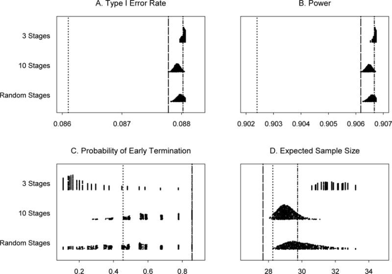
Operating characteristics for 1,000 simulated trials under three scenarios for Example 1: 3 stages, 10 stages, and a random number of stages, all with random cohort sizes. Subpanels: (A) Type I error rates, (B) Power for detecting a response rate of 40%, (C) Probability of early termination if the true response rate is 20% and (D) Expected sample size if the true response rate is 20%. Line types: ……Simon’s minimax two-stage design, -----Predictive probability design, monitoring every patient, -·-·- Predictive probability design, monitoring every 5 patients.

In Example 2 (Section 3.2), under the same evaluation of robustness, almost all the type I error rates are slightly larger than 0.05 and the power values are all higher than 0.80 (see Figure 2). Again, the probability of early termination due to futility is smaller and the expected sample size is larger than those from the original PP design. However, all the probabilities of early termination due to futility in the 10-stage scenario and the majority of the probabilities of early termination in the random-stage scenario are larger than those from Simon’s minimax two-stage design. This causes all the expected sample sizes in the 10-stage scenario and most of the expected sample sizes in the random-stage scenario to be smaller than those from Simon’s minimax two-stage design.

Figure 2.

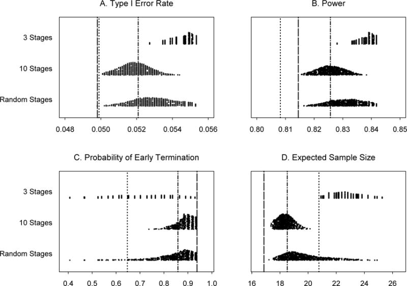
Operating characteristics for 1,000 simulated trials under three scenarios for Example 2: 3 stages, 10 stages, and a random number of stages, all with random cohort sizes. Subpanels: (A) Type I error rates, (B) Power for detecting a response rate of 80%, (C) Probability of early termination if the true response rate is 60% and (D) Expected sample size if the true response rate is 60%. Line types:……Simon’s minimax two-stage design, -----Predictive probability design, monitoring every patient, -·-·- Predictive probability design, monitoring every 5 patients.

When trial conduct deviates from the original design, predictive probability can still be calculated at any time during the trial to provide investigators updated information. The robustness study indicates that the PP design remains robust even when the continuous monitoring rule is not implemented after observing the outcome of every patient. We found that the inflation of the type I error rate is small and usually less than 10% of the pre-specified level in all of our simulation studies.

4.2. Unplanned early termination

Clinical trials can be terminated earlier than planned due to slow accrual or some other reasons. For this situation, we examine the influence of early termination on the design properties. Using our first trial example, presented in Section 3.1, we suppose the trial is stopped after 20 evaluable patients. When θ_T is held at the pre-specified value of 0.922, we will declare that the new regimen is not promising if 6 or fewer responses have been observed in 20 patients, and promising otherwise. The corresponding type I error rate and power are 0.087 and 0.750, respectively. When this unplanned early termination occurs, the type I error rate is still controlled at a level under 10%, whereas power suffers a loss (less than 90%) due to the smaller than planned sample size. Similarly, we assume that the trial is stopped after 20 patients in our second example (Section 3.2). With θ_T =0.963, the type I error rate is controlled at 0.051 (a 2% increase from 0.05) but the power is reduced to 0.630, much less than the targeted 80% level due to the smaller sample size.

4.3. Estimation bias

It is well known that sequential design with outcome-based early stopping rules can result in bias in estimating the parameters corresponding to that outcome. We performed simulation studies to evaluate the bias for Examples 1 and 2 presented in Section 3. Based on 5,000 simulations, the median and mean (standard deviation) of the estimated response rates for Example 1 under p₀ = 0.20 and p₁ = 0.40 are 0.19, 0.17 (0.09) and 0.39, 0.40 (0.09), respectively. For Example 2, the corresponding statistics for the estimated response rates under p₀ = 0.60 mid p₁ = 0.80 are 0.55, 0.55 (0.12) and 0.80, 0.78 (0.10), respectively. Due to the higher probability of early stopping under H₀, the bias is more prominent in H₀ than in H₁. Under H₀, the observed median and mean underestimate the true response rate by about 10%. The early stopping rate under H₁ is low. Hence, less bias is observed in estimating the true response rate.

4.4. Comparison between the designs based on the posterior probability versus designs based on predictive probability

Taking the settings in Examples 1 and 2, we also evaluate the operating characteristics for the designs based on the posterior probability approach. To mimic the aforementioned predictive probability approach, we define the early stopping rule for the posterior probability approach: (1) Stop the trial when P(p > p₁) < θ_* for futility and (2) declare a positive trial at the end of the study when P(p > p₀) > θ*. In the setting of Example 1, with N_max = 36, the corresponding design parameters for the posterior probability approach are θ_* =0.001, θ*= [0.852, 0.922]. The resulting type I error rate, probability of early stopping, and expected sample size under H₀ are 0.088, 0.45, and 28.73, respectively. Under H₁, the study power is 0.905 and the expected sample size is 35.73. These results are quite similar to the predictive probability approach reported in Section 3, except that the probability of early stopping is much lower (0.45 versus 0.86) under H₀.

Another notable difference is the construct of rejection regions. For the posterior probability approach, the rejection region is 0/10, 1/15, 2/20. 3/24, 4/28, 5/32, and 10/36. There is a big jump toward the end of the study (5/32 to 10/36) for the posterior probability approach while the transition for the predictive probability approach is smoother. Similar results are found in Example 2 (data not shown).

5. DISCUSSION

In the frequentist multi-stage design, the study design is rigid in the sense that decisions can only be made at predetermined cohort sizes of the trial. However, the design with the predictive probability approach provides an excellent alternative for conducting multi-stage phase II trials. It is efficient and flexible. The design parameters can be found by searching the parameter space and choosing appropriate values of θ_L and θ_T such that the type I and type II error rates are controlled. The sample size can be determined by choosing the smallest N_max among all designs that satisfy the design criteria. The PP design yields a higher probability of early stopping and a smaller expected sample size compared to Simon’s two-stage designs when the treatment is unlikely to be efficacious. By varying the number of stages and cohort sizes, the PP design also shows robust operating characteristics. When the trial conduct deviates from the original plan, the type I error rate only increases slightly. To ensure that the nominal type I error rate is controlled, we can design the trial with a stricter type I error rate. For example, we can set type I error rates as 0.045 and 0.09 for targeting 0.05 and 0.10 type I error rates, respectively. Furthermore, through the specification of the prior distribution, the PP design can formally incorporate the additional efficacy information obtained before and throughout the trial into the decision making process. The PP design allows for a highly flexible monitoring schedule that is suitable for clinical applications, yet its operating characteristics remain robust. In our trial examples, we monitor the trial continuously after the first 10 patients are treated and are evaluable for response. Although we present the PP design using continuous monitoring, the approach can be applied with any number of stages and cohort sizes. In practice, the first cohort of patients and the number of stages are usually determined after consulting with study investigators to identify a reasonable choice that balances the practical considerations with trial efficiency.

We find that comparable operating characteristics can be obtained by taking both the predictive probability and the posterior probability approaches. However, the predictive probability approach resembles more closely the clinical decision making process, i.e., deciding whether to continue the study based on the interim data, as well as projecting into the future. The predictive probability approach also leads to higher early stopping rates under the null hypothesis (when treatment not working). Furthermore, the rejection region has a smooth transition compared to the posterior probability approach, which is likely to have a “jump” between the interim data analysis and the final analysis. Further research on comparing the applications of the two approaches in designing clinical trials is warranted.

Regarding the choice of θ_L and θ_T: In general, the lower θ_T is, the easier it is to reject H₀, hence, there is increased power and type I error rate. On the other hand, the higher θ_T is, the harder it is to reject H₀, hence, there is decreased power and type I error rate. Likewise, a larger θ_L corresponds to easier stopping due to futility and decreased power and type I error rate, and a smaller θ_L corresponds to the opposites. However, due to the discrete nature of the binomial distribution, for a fixed parameter (e.g., response rate =20%) with a given prior distribution, there may be a range of θ_L and θ_T which gives the same rejection boundaries. In this case, from the trial conduct point of view, it does not matter which values of θ_L and θ_T are used. If a range of θ_L and θ_T exists which satisfies the prespecified constraints, one may choose the midpoint of the range for defining the decision rule using the predictive probability. The effect of varying parameters or the prior distributions can be evaluated accordingly.

Although frequentist approaches have historically dominated the field of clinical trial design and analysis, Bayesian methods provide many appealing properties. These include the ability to incorporate the information obtained before the trial into the study design, to use the information obtained during the trial for monitoring the study, flexibility in trial conduct, and a consistent way for making inference. [38–40,42] Instead of taking an ideological stand of choosing either the Bayesian or frequentist method, we take a pragmatic approach in searching for a better method for evaluating treatment efficacy in the phase II setting. We use the Bayesian framework as a tool to design clinical trials with desirable frequentist properties. [19] Taking the Bayesian approach, we derive an efficient and flexible design. In the meantime, we choose the design parameters (in our case, N_max, θ_L and θ_T) to control the type I and type II error rates under a variety of settings. Several similar approaches of taking the Bayesian framework to achieve good frequentist properties have been proposed in the literature. [43,44] We advocate the use of extensive computation and/or simulation studies to search for the optimal design parameters and to evaluate the design’s operating characteristics. Sensitivity analysis should be conducted to examine how the design parameters influence the design properties. Robustness analysis should also be carried out to study the impact on design properties when the study conduct deviates from the original design. Based on our extensive studies, we conclude that the predictive probability approach offers practical and desirable designs for phase II cancer clinical trials. S-PLUS/R programs can be downloaded from http://biostatistics.mdanderson.org/SoftwareDownload/ to assist in developing a study design using the described predictive probability method.

One reviewer pointed out the limitation of the traditional hypothesis testing framework when designs are constructedwith the primary goal for controlling type I and type II error rates. For example, as shown in Example 2 and Table 3, both Simon’s minimax design and our predictive probability design will reject the null hypothesis if we observe 25 responses in 35 patients when P₀= 0.6, p₁= 0.8, α=0.05, and β=0.2. It seems unreasonable that we fail to reject p₀= 0.6 when the observed response rate $\widehat{p}=0.71$ is considerably larger than 0.6. This is a result of choosing a small type I error rate. To achieve a valid scientific inference, we emphasize the importance of estimation even when the trial is designed under the hypothesis testing framework. In this example, the posterior distribution for the response rate is beta(25.6, 10.4) if we take the prior as beta(0.6, 0.4). The probabilities that the response rate is greater than 0.6 and 0.8 are 0.92 and 0.11, respectively. The 95% highest probability density interval for the response rate is (0.56, 0.85). The posterior probability provides a more thorough assessment of the response rate under the Bayesian framework.

Lastly, we would like to emphasize that reaching an efficacy threshold is not the only purpose of phase II trials. Information collected from phase II studies will enable the investigators to provide further safety analysis, to find out appropriate dosing schedules, to identify appropriate populations for a new treatment, and to assess the possibility for combination studies, etc. Depending on the purpose of the study, the investigators may not always want to terminate the study early, even when the early stopping boundary is crossed. However, the predictive probability approach still offers a consistent way to evaluate the strength of the treatment efficacy based on the observed data. Phase II trials can be considered as learning studies. The predictive probability design under the Bayesian framework provides an ideal environment for learning.

List of abbreviations

E(N)

expected sample size

PET

probability of early termination

PP

predictive probability

References

- 1.Green S, Benedetti J, Crowley J. Clinical trials in oncology. 2nd. Chapman & Hall/CRC; 2002. [Google Scholar]
- 2.Palesch YY, Tilley BC, Sackett DL, Johnson KC, Woolson R. Applying a phase II futility study design to therapeutic stroke trials. Stroke. 2005;36:2410–4. doi: 10.1161/01.STR.0000185718.26377.07. [DOI] [PubMed] [Google Scholar]
- 3.Thall PF, Simon RM. Recent developments in the design of phase II clinical trials. Cancer Treat Res. 1995;75:49–71. doi: 10.1007/978-1-4615-2009-2_3. [DOI] [PubMed] [Google Scholar]
- 4.Kramar A, Potvin D, Hill C. Multistage designs for phase II clinical trials: statistical issues in cancer research. Br J Cancer. 1996;74:1317–20. doi: 10.1038/bjc.1996.537. [DOI] [PMC free article] [PubMed] [Google Scholar]
- 5.Mariani L, Marubini E. Design and analysis of phase II cancer trials: A review of statistical methods and guidelines for medical researchers. Int Stat Rev. 1996;64(1):61–88. [Google Scholar]
- 6.Lee JJ, Feng L. Randomized phase II designs in cancer clinical trials: current status and future directions. J Clin Oncol. 2005;23:4450–7. doi: 10.1200/JCO.2005.03.197. [DOI] [PubMed] [Google Scholar]
- 7.Gehan EA. The determination of the number of patients required in a preliminary and a follow-up trial of a new chemotherapeutic agent. J Chronic Dis. 1961;13:346–53. doi: 10.1016/0021-9681(61)90060-1. [DOI] [PubMed] [Google Scholar]
- 8.Simon R. Optimal two-stage designs for phase II clinical trials. Cont Clin Trials. 1989;10:1–10. doi: 10.1016/0197-2456(89)90015-9. [DOI] [PubMed] [Google Scholar]
- 9.Fleming TR. One-sample multiple testing procedure for phase II clinical trials. Biometrics. 1982;38:143–51. [PubMed] [Google Scholar]
- 10.Lee YJ. Phase II trials in cancer: present status and analysis methods. Drugs Exp Clin Res. 1986;12:57–71. [PubMed] [Google Scholar]
- 11.Ensign LG, Gehan EA, Kamen DS, Thall PF. An optimal three-stage design for phase II clinical trials. Stat Med. 1994;13:1727–36. doi: 10.1002/sim.4780131704. [DOI] [PubMed] [Google Scholar]
- 12.Chen TT. Optimal three-stage designs for phase II cancer clinical trials. Stat Med. 1997;16:2701–11. doi: 10.1002/(sici)1097-0258(19971215)16:23<2701::aid-sim704>3.0.co;2-1. [DOI] [PubMed] [Google Scholar]
- 13.Jung SH, Carey M, Kim KM. Graphical search for two-stage designs for phase II clinical trials. Cont Clin Trials. 2001;22:367–72. doi: 10.1016/s0197-2456(01)00142-8. [DOI] [PubMed] [Google Scholar]
- 14.Jung SH, Lee T, Kim KM, George SL. Admissible two-stage designs for phase II cancer clinical trials. Stat Med. 2004;23:561–9. doi: 10.1002/sim.1600. [DOI] [PubMed] [Google Scholar]
- 15.Green SJ, Dahlberg S. Planned versus attained design in phase II clinical trials. Stat Med. 1992;11:853–62. doi: 10.1002/sim.4780110703. [DOI] [PubMed] [Google Scholar]
- 16.Herndon JE. 2nd: A design alternative for two-stage, phase II, multicenter cancer clinical trials. Cont Clin Trials. 1998;19:440–50. doi: 10.1016/s0197-2456(98)00012-9. [DOI] [PubMed] [Google Scholar]
- 17.Chen TT, Ng TH. Optimal flexible designs in phase II clinical trials. Stat Med. 1998;17:2301–12. doi: 10.1002/(sici)1097-0258(19981030)17:20<2301::aid-sim927>3.0.co;2-x. [DOI] [PubMed] [Google Scholar]
- 18.Korn EL, Simon R. Data monitoring committees and problems of lower-than-expected accrual or events rates. Cont Clin Trials. 1996;17:526–35. doi: 10.1016/s0197-2456(96)00088-8. [DOI] [PubMed] [Google Scholar]
- 19.Berry DA. Introduction to Bayesian methods III: use and interpretation of Bayesian tools in design and analysis. Clin Trials. 2005;2:295–300. doi: 10.1191/1740774505cn100oa. discussion 301–4, 364–78. [DOI] [PubMed] [Google Scholar]
- 20.Berry DA. Clinical trials: is the Bayesian approach ready for prime time? Yes! Stroke. 2005;36:1621–2. doi: 10.1161/01.STR.0000170637.02692.14. [DOI] [PubMed] [Google Scholar]
- 21.Sylvester RJ. A Bayesian approach to the design of phase II clinical trials. Biometrics. 1998;44:823–36. [PubMed] [Google Scholar]
- 22.Thall PF, Simon R. A Bayesian approach to establishing sample size and monitoring criteria for phase II clinical trials. Cont Clin Trials. 1994;15:463–481. doi: 10.1016/0197-2456(94)90004-3. [DOI] [PubMed] [Google Scholar]
- 23.Thall PF, Simon R. Practical Bayesian guidelines for phase IIB clinical trials. Biometrics. 1994;50:337–349. [PubMed] [Google Scholar]
- 24.Heitjan DF. Bayesian interim analysis of phase II cancer clinical trials. Stat Med. 1997;16:1791–802. doi: 10.1002/(sici)1097-0258(19970830)16:16<1791::aid-sim609>3.0.co;2-e. [DOI] [PubMed] [Google Scholar]
- 25.Tan SB, Machin D. Bayesian two-stage designs for phase II clinical trials. Stat Med. 2002;21:1991–2012. doi: 10.1002/sim.1176. [DOI] [PubMed] [Google Scholar]
- 26.Mayo MS, Gajewski BJ. Bayesian sample size calculations in phase II clinical trials using informative conjugate priors. Cont Clin Trials. 2004;25:157–67. doi: 10.1016/j.cct.2003.11.006. [DOI] [PubMed] [Google Scholar]
- 27.Gajewski BJ, Mayo MS. Bayesian sample size calculations in phase II clinical trials using a mixture of informative priors. Stat Med. 2006;25:2554–66. doi: 10.1002/sim.2450. [DOI] [PubMed] [Google Scholar]
- 28.Spiegelhalter DJ, Abrams KR, Myles JP. Bayesian Approaches to Clinical Trials and Health-Care Evaluation. John Wiley & Sons; 2004. [Google Scholar]
- 29.Choi SC, Smith PJ, Becker DP. Early decision in clinical trials when the treatment differences are small. Experience of a controlled trial in head trauma. Cont Clin Trials. 1985;6:280–8. doi: 10.1016/0197-2456(85)90104-7. [DOI] [PubMed] [Google Scholar]
- 30.Choi SC, Pepple PA. Monitoring clinical trials based on predictive probability of significance. Biometrics. 1989;45:317–23. [PubMed] [Google Scholar]
- 31.Spiegelhalter DJ, Freedman LS, Blackburn PR. Monitoring clinical trials: conditional or predictive power? Cont Clin Trials. 1986;7:8–17. doi: 10.1016/0197-2456(86)90003-6. [DOI] [PubMed] [Google Scholar]
- 32.Spiegelhalter DJ, Ereedman LS. A predictive approach to selecting the size of a clinical trial, based on subjective clinical opinion. Stat Med. 1986;5:1–13. doi: 10.1002/sim.4780050103. [DOI] [PubMed] [Google Scholar]
- 33.Grieve AP. Predictive probability in clinical trials. Biometrics. 1991;47:323–30. [PubMed] [Google Scholar]
- 34.Johns D, Andersen JS. Use of predictive probabilities in phase II and phase III clinical trials. J Biopharm Stat. 1999;9:67–79. doi: 10.1081/BIP-100101000. [DOI] [PubMed] [Google Scholar]
- 35.Gould AL. Timing of futility analyses for proof of concept trials. Stat Med. 2005;24:1815–35. doi: 10.1002/sim.2087. [DOI] [PubMed] [Google Scholar]
- 36.Herson J. Predictive probability early termination plans for phase II clinical trials. Biometrics. 1979;35:775–83. [PubMed] [Google Scholar]
- 37.Schultz JR, Nichol FR, Elfring GL, Weed SD. Multiple-stage procedures for drug screening. Biometrics. 1973;29:293–300. [PubMed] [Google Scholar]
- 38.Lee JJ, Tu ZN. A versatile one-dimensional distribution plot: the BLiP plot. The American Statistician. 1997;51:353–358. [Google Scholar]; Spiegelhalter DJ, Ereedman LS, Parmar MKB. Bayesian approaches to randomized trials. Journal of the Royal Statistical Society Series A. 1994;157:357–416. [Google Scholar]
- 39.Grossman J, Parmar MKB, Spiegelhalter DJ, Freedman LS. A unified method for monitoring and analysing controlled trials. Statistics in Medicine. 1994;13:1815–1826. doi: 10.1002/sim.4780131804. [DOI] [PubMed] [Google Scholar]
- 40.Spiegelhalter DJ, Myles JP, Jones DR, Abrams KR. Bayesian methods in health technology assessment: A review. Health Technology Assessment. 2000;4:1–121. [PubMed] [Google Scholar]
- 42.Berry DA. A guide to drug discovery: Bayesian clinical trials. Nature Reviews Drug Discovery. 2006;5:27–36. doi: 10.1038/nrd1927. [DOI] [PubMed] [Google Scholar]
- 43.Stallard N, Whitehead J, Cleall S. Decision-making in a phase II clinical trial: A new approach combining Bayesian and frequentist concepts. Pharmaceutical Statistics. 2005;4:119–128. [Google Scholar]
- 44.Wang YG, Leung DHY, Li M, Tan SB. Bayesian designs with frequentist and Bayesian error rate considerations. Statistical Methods in Medical Research. 2005;14:445–456. doi: 10.1191/0962280205sm410oa. [DOI] [PubMed] [Google Scholar]