A Bayesian approach to identify genes and gene-level SNP aggregates in a genetic analysis of cancer data

Abstract

Complex diseases, such as cancer, arise from complex etiologies consisting of multiple single-nucleotide polymorphisms (SNPs), each contributing a small amount to the overall risk of disease. Thus, many researchers have gone beyond single-SNPs analysis methods, focusing instead on groups of SNPs, for example by analysing haplotypes. More recently, pathway-based methods have been proposed that use prior biological knowledge on gene function to achieve a more powerful analysis of genome-wide association studies (GWAS) data. In this paper we propose a novel Bayesian modeling framework to identify molecular biomarkers for disease prediction. Our method combines pathway-based approaches with multiple SNP analyses of a specified region of interest. The model’s development is motivated by SNP data from a lung cancer study. In our approach we define gene-level scores based on SNP allele frequencies and use a linear modeling setting to study the scores association to the observed phenotype. The basic idea behind the definition of gene-level scores is to weigh the SNPs within the gene according to their rarity, based on genotype frequencies expected under the Hardy-Weinberg equilibrium law. This results in scores giving more importance to the unusually low frequencies, i.e. to SNPs that might indicate peculiar genetic differences between subjects belonging to different groups. An additional feature of our approach is that we incorporate information on SNP-to-SNP associations into the model. In particular, we use network priors that model the linkage disequilibrium between SNPs. For posterior inference, we design a stochastic search method that identifies significant biomarkers (genes and SNPs) for disease prediction. We assess performances on simulated data and compare results to existing approaches. We then show the ability of the proposed methodology to detect relevant genes and associated SNPs in a lung cancer dataset.

1. INTRODUCTION

In disease gene association studies, often repeated univariate methods with multiple comparison corrections are applied to cases and controls to identify variants that relate to a disease, see [24] or [7] among others. However, multivariate methods offer a more powerful unified approach to investigate candidate regions for complex diseases [20, 33, 49]. Multivariate methods allow joint modeling of multiple SNPs to infer associations with disease status and can take advantage of genetic correlation and other biological structures [49, 51]. However, as noted for example by [41], in most situations the identified SNPs from GWAS and/or candiate gene studies have only explained a small part of heritability. A possible explanation for this is genetic heterogeneity, i.e. the fact that different alleles at different loci might contribute to a disease in different populations. Genetic heterogeneity makes it difficult to detect genetic variants with small or moderate individual effects. Other theories attribute the unexplained heritability to gene environment interactions, gene-gene interactions, epistasis, structural variation, and the most popular to rare variants with large effect size [13, 14, 18, 31, 60]. Here we are mainly concerned with the issue of genetic heterogeneity.

In order to address heterogeneity, many researchers have gone beyond single-SNPs analysis methods, focusing instead on groups of SNPs, for example by analyzing haplotypes, i.e., sets of associated SNPs that get transmitted together as a block [11]. More recent gene approaches consider biological/functional information as a component to the investigation, either as a preprocessing step to select candidate genes, or for inclusion in the modeling process or both [7, 20, 51]. Many current methods can also be applied at a second phase, following GWAS. Among recent contributions, [9] adopts a strategy that uses representative eigen-SNPs for each gene to assess their joint association with disease risk, while [10] defines pathway-level latent variables based on principal components analysis applied to subsets of SNPs selected as the most associated with the disease outcome. [39] employs logic regression to sets of SNPs (belonging to the same gene or pathway) in order to identify those genes or pathways comprising SNPs that are most consistently associated with the response. Also, [20] uses a composite likelihood approach assuming a latent Gaussian model underlying the SNP distributions to model cases and controls for a candidate region association test.

Building upon this rich literature, we propose a Bayesian model for the identification of molecular biomarkers (SNPs and genes) for disease prediction using candidate regions. We assume we have data available on p SNPs, typically measured across a population of genetically diverse individuals, as categorical covariates. In similar spirit to some of the contributions described above, we use a linear modeling setting to relate the observed phenotype to summary measures of aggregated SNPs. Our modeling approach is flexible and can incorporate different types of summary scores as a way to aggregate SNP measurements. Here, in particular, we define gene-level scores based on the associated SNP genotypes. The basic idea of the type of scores we incorporate is to weigh the observed SNP genotypes using the genotype frequencies expected under the Hardy-Weinberg equilibrium law. Such a scoring method gives more importance to genotypes that are less common in the population, in effect upweighing SNPs that contribute to risk and would therefore be reduced in the population due to selection pressure. We incorporate latent variables to deal with the binary response variable that represents the phenotype of the cancer patients. For posterior inference, we design a stochastic search method that identifies the significant biomarkers for disease prediction. With respect to other proposed methodologies for the analysis of group-level SNPs data, our method leads to the simultaneous selection of both genes and relevant SNPs associated with the phenotype.

An additional feature of the modeling strategy we use is the incorporation of information on SNP-to-SNP associations into the prior model. In particular, we use network priors that capture non-random associations between pairs of SNPs based on their linkage disequilibrium (LD). In genetics, LD represents genetic correlation stemming from the biological processes of mutation and recombination, and a function of genetic distance between loci. Essentially, for SNPs closer together in terms of genetic distance, some combinations of alleles or genetic markers occur more (or less) frequently in a population than what would be expected from a random formation of haplotypes from these alleles. [49] shows that incorporating LD structure in priors for hierarchical Bayesian models improves power and reduces false positives. In our model, we employ Markov random field (MRF) priors to represent a graph structure among a set of SNPs, with nodes representing SNPs and edges representing relations between the nodes, and use the LD information as the prior strength of the connection between two SNPs. Thus, the prior probability of a SNP to be associated with the phenotype depends on those SNPs in strong LD with it. This also helps identify regions of interest when the true underlying causal SNP is not genotyped, because the signal is largely based on LD between the genotyped SNPs and the untyped causal SNP. Overall, our results suggest that including biological information in the model helps achieve a sharper selection, particularly in situations where the number of causal SNPs is extremely small with respect to the number of non predictive (noisy) SNPs. We empirically demonstrate that our method leads to the inclusion of fewer false positives and gives higher confidence, in terms of posterior probability, in the selection of the true positive casual SNPs.

The remainder of the paper is organized as follows. In Section 2, we discuss the model formulation, the construction of the gene-level scores and the prior network capturing the LD association between SNPs. Section 3 describes the MCMC stochastic search procedure to fit the model and the strategies for posterior inference. In Section 4, we first show the ability of the proposed methodology to detect relevant biomarkers using simulated data and also compare results to existing approaches. We then illustrate an application of the method to the lung cancer data of [2]. We conclude the paper with a brief discussion in Section 5.

2. METHODS

We have available observational data consisting of SNP genotypes and phenotype information on a number of individuals. We aggregate SNPs based on their gene membership and define gene-level scores based on the additively coded SNP genotypes. Our goal is to build a model that identifies genes related to the phenotype while simultaneously locating SNPs from these selected genes that are involved in the biological process of interest. For each gene there is a set of SNPs that belong to it, while every SNP belongs to one gene only. We create gene scores based on the associated SNPs and use a linear modeling framework where the response variable is the observed phenotype and the covariates are the gene-level summary scores.

We capture data and external biological information available to us as follows:

1. Y, an n × 1 binary outcome vector indicating the subjects’ phenotype.

2. X, an n × p matrix of genotypes.

3. S, a K × p matrix indicating membership of the p SNPs to K genes, with element s_kj = 1 if SNP j belongs to gene k, and s_kj = 0 otherwise.

4. R, a p × p matrix describing relationships between SNPs, with element r_ij > 0 if SNPs i and j have a direct association, and r_ij = 0 otherwise, where r_ij is the value of LD estimated from Haploview 4.2 of [5].

Matrices S and R are constructed using available genetic information. The matrix S can be easily defined using information from the National Center for Biotechnology Information’s (NCBI) dbSNP database. This database lists every discovered SNP by its RS identification number and contains information on SNP memberships to genes. The matrix R captures a graph where SNPs form a network of connected elements. Here we base the structure of the network on the amount of linkage disequilibrium between the SNPs. LD refers to the genetic correlation between loci (SNPs or genes) stemming from the original mutation occurring on a single chromosome. LD decays over time, slowly, depending on the genetic recombination between the mutation and other nearby loci [21, 42]. In this paper, we essentially look at LD as the correlation between two genetic loci and use it to define a prior structure where we consider two SNPs connected if the amount of LD is greater than a threshold, τ. Previous work using hierarchical models has shown that it is advantageous to model LD when the LD is greater than 0.25, see [48]. In the applications presented later we therefore set the threshold τ at 0.25.

Let T(n × K) be the matrix of gene-level summary measures of SNP measurements. In Section 2.1 below we describe a particular type of score we will adopt in this application. We consider a probit model that linearly relates the gene scores to the binary response variable Y representing the patients’ phenotype. We adopt the data augmentation approach of [1] and write

$$\begin{array}{cc}{z}_i=\alpha +{\displaystyle \sum _{k=1}^K{T}_{ik}{\beta }_k+{\epsilon }_i,}& {\epsilon }_i\end{array}~N(0,{\sigma }^2),$$ (1)

for i = 1,…, n, where z_i is a latent variable, capturing the unobserved propensities of subject i to belong to one of the two classes, which is linked to the observed y_i as follows:

$$y_i=\{\begin{array}{ll}0\hfill & \text{if}{z}_i<0\hfill \\ 1\hfill & \mathit{otherwise}\hfill \end{array}.$$ (2)

It is evident that multiplying α and β by a constant c and σ by the same constant leaves the model unchanged. Thus the constraint σ² = 1 is often used to identify the model. The construction easily extends to multinomial responses, see [1]. In order to ensure identifiability we need to ensure that the covariates T_ik’s in our model are not identical. We achieve this by imposing that each covariate is a function of a distinct set of SNPs, see also [47].

2.1 Covariates as gene-level SNP aggregates

Our modeling approach is general and can accommodate different types of gene-level scores. Here we create gene-level scores of SNP aggregates by using weighted averages of the SNP genotypes under an additive coding. For each SNP, the genotype is coded by the number of a prespecified allele, usually the minor allele. Thus each SNP genotype has the value of 0, 1, 2. At this stage we want the less common genotypes to more strongly affect the gene scores than the more common genotypes. We achieve this goal by weighing the SNP genotypes according to their expected proportions calculated under the Hardy-Weinberg equilibrium law. Thus, by construction, our scoring method gives more importance to the less common alleles or genotypes, i.e. to the SNPs that might indicate peculiar genetic differences between subjects belonging to different groups. This weighted average of SNPs within genes allows us to deal with count variables while at the same time preserving most of the information carried by the entire initial set of variables, as also noted by [12]. Thus, for gene k we construct an n × 1 vector T_k of scores calculated based on the vectors X_is of SNP genotypes belonging to gene k, encoded by the matrix S, as

$$T_{ik}={\displaystyle \sum _{j=1}^{p_k}{w}_{ij}{X}_{ij}},$$ (3)

where we define the weights w_ij as

$${\stackrel{\sim }{w}}_{ij}=\pi \frac{1}{f_{ij}}+(1-\pi )\frac{1}{p_k},w_{ij}={\stackrel{\sim }{w}}_{ij}/{\displaystyle \sum _j{\stackrel{\sim }{w}}_{ij}}$$ (4)

with f_ij, the expected population genotype frequencies computed according to the Hardy-Weinberg law using the allele frequencies (readily available as part of the annotation files of any standard GWAS chip); p_k, the number of SNPs in gene k; and π, a constant between 0 and 1 determining the influence of the Hardy-Weinberg frequencies on the gene scores. Notice how weights w_ij’s assume higher values for less common genotypes and smaller values for more common genotypes. In the applications section below we give more details on choosing π.

Similar weights to those we have defined in (4) have been used with genotype data by other authors, though in very different contexts. For example, [30] proposes a weighted-sum method to jointly analyze a group of mutations in order to test for groupwise association with disease status. [27] defines a kernel to measure the genomic similarity between two subjects. In our definition, the weight is genotype specific, rather than locus specific. Also, construction (4) allows the weight to be a weighted average of constant weights and weights based on the genotype frequency, via the parameter π.

2.2 Variable selection priors

We want to identify genes related to the phenotype while simultaneously locating SNPs from these selected genes that are involved in the biological process of interest. We introduce two binary vectors, θ and γ, for gene and SNP selection, respectively. For included genes, scores are then calculated using only the selected SNPs. In other words, we re-write model (1) as

$$\begin{array}{cc}{z}_i=\alpha +{\displaystyle \sum _{k=1}^{K_{\theta }}{T}_{ik(\gamma )}{\beta }_{k(\gamma )}+{\epsilon }_i},& {\epsilon }_i~N(0,1),\end{array}$$ (5)

for i = 1,…, n, where $K_{\theta }={\displaystyle {\sum }_{k=1}^K{\theta }_k}$ is the number of genes included in the model. The subscript k(γ) indicates that scores for gene k are calculated based on the subset of SNPs identified by the elements of γ equal to 1. This model formulation allows us to study the association between the response variable and the selected genes and related SNPs, simultaneously. We use θ_k to specify a mixture prior of a normal density and a point mass at zero on β_k, similar to the spike and slab approach for variable selection of [17], also applied to genetics in [19],

$${\beta }_k|{\theta }_k~{\theta }_k\cdot N({\beta }_0,h)+(1-{\theta }_k)\cdot {\delta }_0({\beta }_k),$$ (6)

for k = 1,…, K, with δ₀(β_k) the Dirac Delta function. The hyperparameter h in (6) induces shrinkage in the model. We follow the guidelines provided by [40] and [26] and specify h in the range of variability of the data so as to control the ratio of prior to posterior precision. For the intercept term, α, we take a conjugate prior, α ~ N(α₀, h₀), with α₀ and h₀ to be elicited.

Let us now define the prior distributions for the selection indicators θ and γ. We first define them marginally, and then jointly, taking into account some necessary constraints. We assume independent Bernoulli priors for the θ_k’s,

$$p(\theta |\phi )={\displaystyle \prod _{k=1}^K{\phi }_k^{{\theta }_k}{(1-{\phi }_k)}^{1-{\theta }_k}},$$ (7)

with φ_k the proportion of genes expected a priori to be included in the model. In applications, when using specification of the type φ_k = φ we noticed that genes with a large number of SNPs tended to be visited more often than sets with a smaller number of elements. We therefore decided to penalize the prior probability of gene inclusion as a function of the number of SNPs for each gene (L_k), by defining ${\phi }_k=\frac{L_{\mathit{max}}}{L_k}{\phi }_0$ with L_max = max_r L_r and φ₀ a very small constant that can be chosen according to the a priori expected number of relevant genes. This specification results in ϕ_k being a decreasing function of L_k. This formulation offers some adjustment for gene size. In particular, since the number of possible configurations of selected SNPs for each gene, $n_c={\displaystyle {\sum }_{l=1}^{L_r}\left({}_l^{Lr}\right)}$, depends on the number of SNPs, L_r, that belong to that gene, our method avoids assigning similar prior probabilities to two genes of very different sizes. Notice how, of course, our prior specification will assign rather small probabilities to configurations with a very large number of selected SNPs.

The subset of selected SNPs is identified by the elements of γ equal to 1, whereas we set w_i,j = 0 when γ_j = 0. Note that only the subset of selected SNPs contributes to (3), and that p_k in (4) is set to the number of selected SNPs for gene k. For the latent p-vector γ, we specify a prior distribution that captures biological relationships between SNPs based on linkage disequilibrium, accounting for the difference between observed and expected allelic frequencies, as encoded by the matrix R. We capture these relations using a Markov random field (MRF) prior distribution of the type

$$P(\gamma |\theta ,\mu ,\eta )\propto \text{exp}(\mu 1_p^{\prime }\gamma +\eta {\gamma }^{\prime }R\gamma ),$$ (8)

with 1_p the unit vector of dimension p and where the unknown normalizing constant is a function of μ, η, θ, and R. A MRF distribution describes, in particular, an undirected graph where pairs of nodes that are not connected are considered conditionally independent given all other nodes [6]. MRF models have recently found useful applications in the modeling of high-throughput data, particularly gene expression data [28, 47, 56]. For GWAS data, [29] proposed a hidden MRF model based on a weighted LD prior graph that assigns posterior probabilities of individual SNPs to be associated with the disease.

The parameter μ in (8) represents the expected prior number of significant SNPs and controls the sparsity of the model, while η affects the probability of selecting a variable according to its neighbor values. This is more evident by noting that the conditional probability

$$P({\gamma }_j|\mu ,\eta ,{\gamma }_k,k\in N_j)=\frac{\text{exp}({\gamma }_j(\mu +\eta {\displaystyle {\sum }_{k\in N_j}{\gamma }_k}))}{1+\text{exp}(\mu +\eta {\displaystyle {\sum }_{k\in N_j}{\gamma }_k})},$$ (9)

with N_j the set of direct neighbors of variable j in the MRF, increases as a function of the number of selected neighbors. Note that if a variable does not have any neighbor, then its prior distribution reduces to an independent Bernoulli with probability of success exp(μ)/[1 + exp(μ)], which is a logistic transformation of μ. We provide some guidelines for choosing the μ and η parameters in the simulation study when we also perform a sensitivity analysis.

Some constraints need to be imposed to ensure interpretability of the model. Essentially, given the way we have defined our model (5), we want to avoid empty covariates, that is, the selection of a gene when none of its SNPs are included in the model, as well as orphan SNPs, that is, the selection of a SNP when the corresponding gene is not included. These constraints imply that some combinations of θ and γ values are not allowed. Taking into account these constraints, we write the joint prior probability for (θ, γ) as

$$\pi (\theta ,\gamma |\eta )\propto \{\begin{array}{c}\underset{\text{for valid configurations,}}{{\displaystyle {\prod }_{k=1}^K{\phi }_k^{{\theta }_k}{(1-{\phi }_k)}^{1-{\theta }_k}\text{exp}(\mu 1_p^{\prime }\gamma +\eta {\gamma }^{\prime }R\gamma )}}\\ \begin{array}{cc}0& \text{for invalid configurations}\end{array}\end{array}.$$ (10)

2.3 Posterior inference

For posterior inference, our major interest is in the selection parameters, that is in the posterior distribution p(γ, θ|T, Y). We therefore integrate out the regression parameters α and β from (5), obtaining a multivariate normal marginal likelihood. Below we briefly describe a Markov Chain Monte Carlo (MCMC) stochastic search algorithm that we designed to sample from the posterior distribution. Full details are given in the Appendix. We also show how to use the MCMC draws to select relevant genes and SNPs and to assess uncertainty on the selection.

Bayesian stochastic variable selection methods have been successfully employed by many authors for the analysis of individual-level SNP data, particularly in genetic association studies [16, 46, 49, 50] and for the detection of rare variants [38, 58]. Stochastic search variable selection (SVSS) is an attractive form of variable selection for several reasons. [50] demonstrates that in simulated case-control association studies, SSVS has greater accuracy than standard variable selection methods such as forward, backward, or stepwise selection. As for GWAS studies, [45] obtains superior performance of SVSS when compared to a penalized sparse regression method, and [19] shows via simulations that, in spite of the apparent computational challenges, SVSS produces better power and predictive performance when compared with standard lasso techniques.

Our MCMC scheme consists of two steps:

1. This step explores the model space in order to find relevant genes and SNPs. At every iteration the parameters θ and γ are updated by deleting or removing one gene and/or one SNP via a two-stage Metropolis-Hastings sampling scheme. For interpretability, as previously described, no empty genes or orphan SNPs are proposed during sampling. At this step we randomly choose one of the following move types:

   • (1a)
     Change the inclusion status of both a gene and a SNP – randomly choose between adding or removing a gene and a SNP.
   • (1b)
     Change the inclusion status of a SNP but not a gene – randomly choose between adding or deleting a SNP from an already included gene.

2. This step generates the latent variable z_i’s from truncated normal distributions under the constraint defined by equation (2).

The MCMC sampler results in a list of sets of included genes and SNPs, together with their corresponding relative posterior probabilities. Important genes can then be selected looking at the marginal posterior probabilities p(θ_k|T, Y), estimated by the relative frequency of inclusion of gene k in the models visited by the MCMC sampler. These marginal posterior probabilities induce a ranking of the genes, so that important ones can be selected by choosing a threshold. Then, relevant SNPs from the selected genes can be identified based on their marginal posterior probabilities, conditional on the inclusion of a set of genes of interest, calculated as p(γ_j|T, Y, I{Σ_kθ_ks_kj = 1}).

3. RESULTS AND DISCUSSION

We first validated our approach through simulations and then applied the methodology to detect relevant genes and associated SNPs in a lung cancer dataset. In the simulations we considered data that mimic the characteristics of SNPs allele frequencies. In particular, we focus here on situations where most of the SNPs are not predictive, to test the ability of our method to discover relevant covariates in the presence of a good amount of noise.

3.1 Simulation study – scenario 1

Using the simuPOP script of [34] and [35], we sampled SNPs from HapMap Phase II data from a 4.4MB region of chromosome 2. These genotypes mimic SNPs found on the human hap 550 chip. We simulated 2000 cases and 2000 controls. We simulated disease status using a single locus with an odds ratio of 1.5 for the minor allele (coded as additive). The minor allele frequency for our SNP was 0.175. The LD of this region for surrounding markers ranged from 0.04–0.76 (based on the R² measure for LD). All SNPs in this region had minor allele frequencies ranging from rarer (0.01) to common (0.49). A total number of 1001 SNPs across 18 genes was used in the simulation.

We report results obtained by choosing, when possible, hyperparameters that lead to weakly informative prior distributions. A vague prior was assigned to the intercept parameter α by setting h₀ to a very large value. For the β_k regression coefficients we set the prior mean to 0 and chose h in the range of variability of the covariates. Specifically, we set h₀ = 10⁴, α₀ = β₀ = 0, and h = 0.5. For the gene selection indicators θ_k we set φ₀ = 0.0001, a value implying that a priori we expect to select approximately one gene. As for the prior at the SNP level, we set μ = −4.5, which corresponds to setting the proportion of SNPs expected a priori to be included in the model to approximately 1%. Parameters φ₀ and μ influence the sparsity of the model and consequently the magnitude of the marginal posterior probabilities. Some sensitivity to the choice of these parameters is, of course, to be expected. However, in our simulations we have noticed that the ordering of genes and SNPs based on posterior probability remains roughly the same and therefore the final selections are unchanged as long as one adjusts the threshold on the posterior probabilities. See also comments in the Discussion section. We set η = 0.05. This parameter controls the prior probability of selecting a SNP based on how many of its neighbors are selected. Finally, we considered three alternative setting for the parameter π:

1. π = 0. In this case the Hardy-Weinberg frequencies do not enter into the calculation of the weights (4) that determine the gene scores.

2. π = 0.5. In this case the weights are an arithmetic mean of the Hardy-Weinberg frequencies and the constant weights.

3. π = 1. In this case the weights are completely determined by the Hardy-Weinberg frequencies.

Two MCMC samplers were run for 200,000 iterations with the first 50,000 used as burn-in. In order to assess the agreement between the two chains, we looked at the correlation between the marginal posterior probabilities for gene selection, p(θ_k|T, Y), for the two chains and found good concordance, with correlation coefficients of 0.99, 0.99 and 0.93 for π = 0, π = 0.5 and π = 1, respectively. Samples from the two chains were then pooled together to perform final inference. We computed the marginal posterior probabilities for gene selection, p(θ_k = 1|Y, T), and the conditional posterior probabilities for SNP selection given a subset of selected genes, p(γ_j|T, Y, I{Σ_kθ_ks_kj = 1}). Figure 1 shows the marginal probabilities for gene selection and Figure 2 the marginal probabilities for SNP selection, conditional upon the inclusion of genes with a marginal probability greater than 0.5 (selected from Figure 1).

Figure 1.

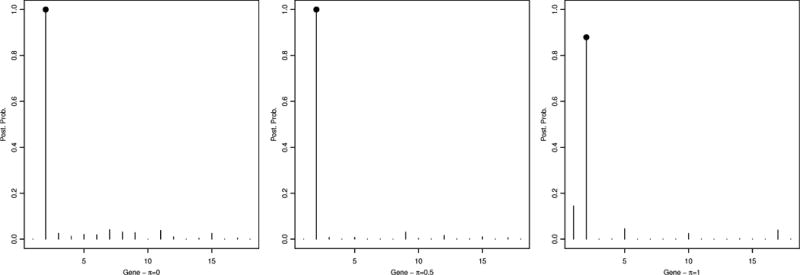
Simulated data – scenario 1: Marginal posterior probabilities for gene selection, p(θ_k|T, Y), for π = 0 (left), π = 0.5 (center) and π = 1 (right).

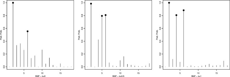
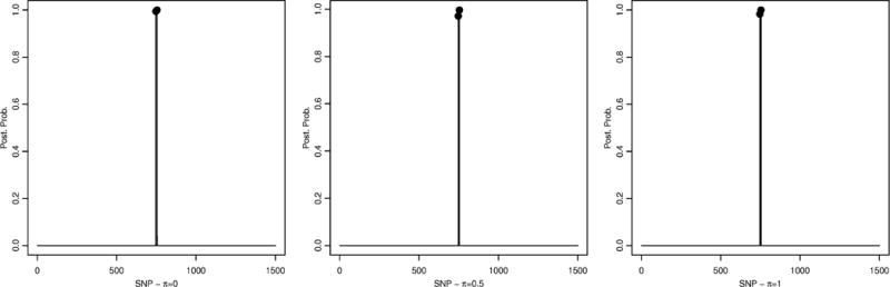
Figure 2.

Simulated data – scenario 1: Conditional posterior probabilities for SNP selection, p(γ_j|T, Y, I{Σ_k θ_ks_kj = 1}), for π = 0 (left), π = 0.5 (center) and π = 1 (right).

A threshold of 0.5 on the marginal posterior probability of gene inclusion correctly identified gene 2 for all cases, with a posterior probability of 0,99, 0,99 and 0.88, for π = 0, π = 0.5 and π = 1, respectively. Also, the true significant SNP, which was SNP 427, belonging to gene 2, was correctly selected by our method with a posterior probability of 0.53, 0.53 for π = 0 and π = 0.5, respectively, see Figure 2. For π = 1, even though the posterior probability was 0.46, below our threshold of 0.5 the SNP was among the top ranked SNPs in the analysis and can be considered as noteworthy. In addition, in the case π = 0 SNPs 428 (p(γ_j|·) = 0.52) and 374 (p(γ_j|·) = 0.32) were also identified, while only SNP 428 was identified in the cases π = 0.5 (p(γ_j|·) = 0.48) and π = 1 (p(γ_j|·) = 0.52). Notice that SNP 428 is adjacent to the causal SNP, therefore lying in the true genetic region. Our results, overall, suggest that the inclusion of biological information in the model helps achieve a sharper selection, as it leads to the inclusion of fewer false positives. Table 1 shows specificity and sensitivity of SNP selection for the three π values using a threshold of 0.45 on the posterior probability.

Table 1.

Comparison of sensitivity (SE) and specificity (SP) for SNP selection for the proposed method and 3 existing approaches, the Bayesian Variable Selection Regression (BVSR) approach for GWAS of [19], the PLINK method of [37] and the Bayesian Hierarchical Generalized Linear Model (BhGLM) approach of [59]

	Scenario 1		Scenario 2
	SE	SP	SE	SP
Our method - π = 0	1.000	0.999	1.000	1.000
Our method - π = 0.5	1.000	0.999	0.400	1.000
Our method - π = 1	1.000	0.999	0.600	0.999
BVSR	1.000	0.999	0.600	1.000
PLINK	1.000	0.998	0.800	0.986
BhGLM - probit link	0.000	0.999	0.600	0.999
BhGLM - logit link	0.000	0.999	0.200	0.997

For comparison, we analyzed the simulated data with the Bayesian Variable Selection Regression (BVSR) approach for GWAS of [19], the PLINK method of [37] and the Bayesian Hierarchical Generalized Linear Model (BhGLM) approach of [59]. BVSR performs multi-SNPs association analysis, either genome-wide or on a small region, and provides marginal posterior inclusion probabilities of each SNP. PLINK, probably the most common method for analyzing GWAS data, computes p-values using univariate logistic regressions for each SNP in the dataset. Finally, BhGLM provides a Bayesian framework for generalized linear models that can simultaneously analyze multiple genetic loci and their association with a disease. Using priors from the t-family (including Cauchy), the method essentially shrinks the parameters of unimportant loci towards 0, through appropriate choices of the scale parameter of the prior. The smaller the scale parameter, the stronger the shrinkage effect. Thus, when investigating multiple loci, small values of the scale parameter essentially control the false discovery rate. All these methods are not designed to perform inference at the gene level and, therefore, we can only compare results on the selection of the SNPs. Applied to our simulated data, BVSR resulted in the selection of SNPs 427 and 428 with posterior probability of 0.51 and 0.49, respectively. Posterior probabilities for all the other SNPs were below 0.1. The PLINK method (version 1.07) found SNPs 427, 428, and 942 as significant after multiplicity correction. For the BhGLM method, we used a Cauchy prior with a scale parameter of 2.5∗10⁻⁴ to control for false positives. BhGLM with a logit link detected SNP 428, which is in high LD with the true SNP 427, therefore this method successfully found the genetic locus. It did not have any false positives. Moreover, we analyzed the simulated data with the probit link and obtained the same results. Table 1 summarizes our comparative analysis. BVSR and PLINK performed equally well both in terms of specificity and sensitivity, whereas BhGLM did not achieve the same performance.

We looked into the sensitivity of our results to the prior choice, in particular by letting η vary in the range 0 to 0.1. Generally speaking, allowing η to vary can lead to phase transition, a situation in which the expected number of variables equal to 1 increases massively for small increments of η, as described, for example, by [28]. Phase transition has consequences, such as the loss of model sparsity, and consequently a critical slow down of the MCMC. In Bayesian variable selection with large p, phase transition leads to a drastic change in the proportion of included variables, for example, from < 5% to > 90%, near the phase transition boundary. The most effective way to obtain an empirical estimate of the phase transition value is to sample from (8), using the algorithm proposed by [36] to obtain an estimate of the expected model size for different values of μ over a range of values for η. The value of η for which the expected model size shows a dramatic increase can be considered a good estimate of the phase transition point. In our case, for π = 0 we observed good robustness of the posterior inference in terms of selected genes and SNPs, for all values of η we considered. For π = 1 a strong prior weight is given to the Hardy-Weinberg frequencies, in addition to the prior on the amount of linkage disequilibrium between SNPs. In this case, when varying η, the method was still able to select the relevant gene 2, suggesting overall robustness to strongly informative prior distributions, although we observed that the posterior probability of gene 1 noticeably increased, lying in the range 0.37–0.49. For π = 0 a higher value of η resulted in larger values of the posterior probability of the false positive SNP 374 (0.38–0.49). Some sensitivity to the choice of μ and φ₀ is, of course, to be expected. However, in our simulation s we have noticed that the ordering of genes and SNPs based on posterior probability remains roughly the same and therefore the final selections are unchanged as long as one adjusts the threshold based on top SNPs ranked by the posterior probability.

3.2 Simulation study – scenario 2

We considered a second simulation scenario where, using the same allele frequencies of Section 3.1, we induced disease status at five loci by setting the odds ratios based on the presence of the minor allele (coded as additive) to, respectively, 1.5, 1.65, 1.5, 1.65 and 1.42. Note that these odds ratios correspond, in the logistic regression used to generate the simulated disease status, to regression coefficients of 0.4, 0.5, 0.4, 0.5 and 0.35. The minor allele frequency for our 5 SNPs were 0.042, 0.007, 0.091, 0.105 and 0.111. The first two causal SNPs are located in a region that corresponds of gene number 2 and the other three in a region that corresponds to gene number 6. All SNPs in this region had minor allele frequencies ranging from rarer (0.01) to common (0.49). A total number of 1001 SNPs across 18 genes was used in the simulation. This simulation scheme led to 1149 cases, we then randomly selected the same numbers of controls in order to define a balanced sample of 2298 units.

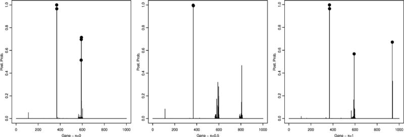
We report results obtained by choosing the same hyperparameter setting of Section 3.1. We considered three alternative settings for π, that is π = 0, 0.5, 1. Two MCMC samplers were run for 200,000 iterations with the first 50,000 used as burn-in. In order to assess the agreement between the two chains, we looked at the correlation between the marginal posterior probabilities for gene selection, p(θ_k|T, Y), for the two chains and found good concordance, with correlation coefficients of 0.72, 0.79 and 0.99 for π = 0, π = 0.5 and π = 1, respectively. Samples from the two chains were then pooled together to perform final inference. We computed the marginal posterior probabilities for gene selection, p(θ_k = 1|Y, T), and the conditional posterior probabilities for SNP selection given a subset of selected genes, p(γ_j|T, Y, I{Σ_kθ_ks_kj = 1}). Figure 3 shows the marginal probabilities for gene selection and Figure 4 the marginal probabilities for SNP selection, conditional upon the inclusion of genes with a marginal probability greater than 0.5 (selected from Figure 3).

Figure 3.

Simulated data – scenario 2: Marginal posterior probabilities for gene selection, p(θ_k|T, Y), for π = 0 (left), π = 0.5 (center) and π = 1 (right).

Figure 4.

Simulated data – scenario 2: Conditional posterior probabilities for SNP selection, p(γ_j|T, Y, I{Σ_k θ_ks_kj = 1}), for π = 0 (left), π = 0.5 (center) and π = 1 (right).

A threshold of 0.5 on the marginal posterior probability of gene inclusion correctly identified gene 2 and 6 for all cases, with a posterior probability of (0.99,0.55), (0.99,0.81) and (0.99,0.88), for π = 0, π = 0.5 and π = 1, respectively. Our approach resulted in a false positive for π = 1, gene 4 with posterior probability of 0.80, and for π = 0.5, gene 5 with posterior probability of 0.80. As for SNP selection, most of the true significant SNPs, which were SNPs 368 and 369, belonging to gene 2, and SNPs 590, 591 and 592, belonging to gene 6, were correctly selected by our method: SNPs 368, 369, 590, 591 and 592 were selected with a posterior probability of 1.00, 0.96, 0.51, 0.70 and 0.71 for π = 0, SNPs 368 and 369 were selected with a posterior probability of 1.00 and 0.99 for π = 0.5, and SNPs 368, 369 and 592 were selected with a posterior probability of 1.00, 0.96 and 0.57 for π = 1, see Figure 4. In addition, in the case π = 1, SNP 938 (p(γ_j|·) = 0.67) was also identified. No false positive SNPs were selected in the case π = 0 and π = 0.5. Table 1 shows specificity and sensitivity of SNP selection for the three π values using a threshold of 0.45 on the posterior probability. These results suggest that the best configuration is when π = 0. This is not surprising since the generating mechanism used to simulate the data implicitly assumes that the gene scores are an equally weighted combination of the true SNPs, i.e. constant w_ij’s.

For comparison, we analyzed our second simulated dataset using the same methods mentioned above: BVSR of [19], PLINK of [37] and BhGLM of [59]. SNPs 368, 590 and 592 were correctly identified by BVSR with posterior probability of 0.93, 0.80 and 0.70. Posterior probabilities for all the other SNPs were below 0.3. After running PLINK, we found SNPs 368, 369, 590 and 591 significant after multiplicity correction. Fourteen false positive SNPs were also selected by PLINK. BhGLM with the logit link only detected SNP 369 of the simulated SNPs and missed the others. In addition, it falsely detected three other SNPs that were not in LD with the true simulated SNPs. However, BhGLM with the probit link gave improved results; it identified SNPs 368, 369 and 590 and only one false positive, but still missed SNPs 591 and 592. Regarding SNP selection, Table 1 shows that the proposed method performs very well for π = 0 and similarly to the BVSR approach and PLINK for π = 0.5, 1.

Given the selected SNPs identified by BVSR, PLINK and BhGLM we used an hypergeometric test in order to identify genes related to the phenotype. Of the two known casual genes, gene 2 was not significant for BVSR (p = 0.31), PLINK (p = 0.88) and BhGLM (p = 0.47 with logit and p = 0.15 with probit link) and gene 6 was found significant for BVSR (p < 0.0001), PLINK (p = 0.01), and BhGLM with probit link (p = 0.01) but not for BhGLM with logit link (p = 0.15). Regarding gene selection, we can then conclude that our approach not only provides a framework that, contrary to any two-step procedure, does not underestimate uncertainty but also results in better sensitivity. We repeated our analysis for several values of μ, set between −4.5 and 4, and of φ₀, set to a value in the 0.001–0.00001 range, and observed that these settings lead to only one or two false discovered genes and one or two false discovered SNPs. Moreover, we have performed additional sensitivity analysis for the parameters h and η: Table 2 shows that sensitivity and specificity of the proposed method are not strongly affected by h and η as long as these parameters are set within the 0.1–0.5 and 0.05–0.1 range, respectively. We notice that SNP sensitivity can be slightly affected by the specification of h and η, whereas gene sensitivity and specificity and SNP specificity are more robust. When different configurations of the hyperparameters lead to different results, it is possible to compute the widely applicable information criterion (WAIC), introduced by [54] and also known as the Watanabe-Akaike information criterion. WAIC is a fully Bayesian approach for estimating the out-of-sample expectation, and its scale is comparable with AIC, DIC, and other measures of deviance. Models with a smaller values of the WAIC should then be preferred. We report the WAIC values for each scenario in the last column of Table 2.

Table 2.

Simulated data – scenario 2: Sensitivity (SE) and specificity (SP) for gene and SNP selection for the proposed method and the Watanabe-Akaike information criterion (WAIC)

	Gene selection		SNP selection		WAIC
	SE	SP	SE	SP
π = 0, h = .5, η = .1	1.000	1.000	0.800	1.000	582.8
π = 0, h = .1, η = .05	1.000	0.936	1.000	0.999	574.1
π = 0, h = .1, η = .1	0.500	0.875	0.400	0.998	603.6
π = .5, h = .5, η = .1	1.000	0.936	0.400	0.999	588.9
π = .5, h = .1, η = .05	1.000	0.875	0.400	0.999	593.1
π = .5, h = .1, η = .1	1.000	0.936	0.400	0.999	579.1
π = 1, h = .5, η = .1	1.000	0.875	0.600	0.999	585.9
π = 1, h = .1, η = .05	1.000	0.936	0.600	0.999	585.3
π = 1, h = .1, η = .1	1.000	0.936	0.600	0.999	584.9

3.3 Simulation study – scenario 3

We considered a third simulation scenario where, using the same allele frequencies of Section 3.1, we induced disease status at seven loci by setting the odds ratios based on the presence of the minor allele (coded as additive) to, respectively, 2.0, 2.1, 2.2, 0.45, 0.50, 0.45, and 0.50. The minor allele frequency for our 7 SNPs were 0.042, 0.007, 0.009, 0.064, 0.247, 0.291, and 0.204. The first two causal SNPs are located in a region that corresponds to gene number 2, the third SNP is located in a region that corresponds to gene 1, the fourth and fifth SNPs are located in a region that corresponds to gene 3, and the other two in a region that corresponds to gene number 4. A total number of 1001 SNPs across 18 genes was used in the simulation. To assess uncertainty about our estimation results, we performed inference for 25 simulated data sets, generated using the same procedure as above.

We report results obtained by choosing the same hyper-parameter setting as in Section 3.1. MCMC samplers were run for 200,000 iterations with the first 50,000 used as burn-in. We computed the marginal posterior probabilities for gene selection and the conditional posterior probabilities for SNP selection given a subset of selected genes. As the generating process used to simulate the data does not account for the expected population genotype frequencies derived by the Hardy-Weinberg Law, we decided to analyze the data setting π = 0. Overall, PLINK, BVSR, and the proposed method performed much better than BhGLM, both with probit and logit link. Our method performed similarly to PLINK and BVSR in terms of TPR and FPR for SNP selection and outperformed the other methods in terms of TPR for gene selection, and had an higher FPR in terms of gene selection compared to BVSR and PLINK, see Table 3. Specifically, PLINK performs very well in terms of TPR for SNPs but yields a very large number of false positive SNPs (40 on average). Moreover, a closer look to the false discovered SNPs by our method reveals that almost half of them are located in regions very close (±3 base pairs) to the true SNPs. Finally, Table 3 shows that both BVSR and our approach have a very good specificity in terms of SNP selection. The very good performance of BVSR are not surprising as the generating process used to produce the simulated data perfectly matches the model assumptions of BVSR. A ROC analysis confirms that the proposed method works very well in terms of gene selection, and that BVSR and PLINK work very well in terms of SNP selection, see Table 4.

Table 3.

Simulated data – scenario 3: Comparison of mean true positive rate (TPR) and false positive rate (FPR) and their standard errors (se) over 25 replicates for gene and SNP selection, for the proposed method and three existing approaches, the Bayesian Variable Selection Regression (BVSR) approach for GWAS of [19], the PLINK method of [37] and the Bayesian Hierarchical Generalized Linear Model (BhGLM) approach of [59]

	Gene selection
	TPR (se)	FPR (se)
Our method - π = 0	0.99 (0.05)	0.12 (0.06)
BVSR	0.72 (0.08)	0.01 (0.01)
PLINK	0.64 (0.12)	0.05 (0.05)
BhGLM - probit link	0.90 (0.12)	0.78 (0.09)
BhGLM - logit link	0.89 (0.13)	0.67 (0.11)

	SNP selection
	TPR (se)	FPR (se)
Our method - π = 0	0.72 (0.14)	0.002 (0.002)
BVSR	0.78 (0.14)	0.001 (0.001)
PLINK	0.80 (0.11)	0.040 (0.004)
BhGLM - probit link	0.38 (0.16)	0.123 (0.016)
BhGLM - logit link	0.36 (0.17)	0.066 (0.010)

Table 4.

Simulated data – scenario 3: Comparison of the area under the curve (AUC) and their standard errors (se) over 25 replicates for gene and SNP selection, for the proposed method and three existing approaches, the Bayesian Variable Selection Regression (BVSR) approach for GWAS of [19], the PLINK method of [37] and the Bayesian Hierarchical Generalized Linear Model (BhGLM) approach of [59]

	Gene	SNP
	AUC (se)	AUC (se)
Our method - π = 0	0.997 (0.008)	0.930 (0.055)
BVSR	0.983 (0.047)	0.999 (0.001)
PLINK	0.929 (0.048)	0.976 (0.004)
BhGLM - probit link	0.559 (0.074)	0.669 (0.106)
BhGLM - logit link	0.611 (0.077)	0.740 (0.112)

3.4 Lung cancer study

[2] conducted a genome-wide association study of histologically confirmed non-small cell lung cancer to identify common low-penetrance alleles influencing lung cancer risk. To minimize confounding effects from cigarette smoking and increase the power to detect genetic effects, they frequency matched controls to cases according to smoking behavior. Also, to minimize confounding by ethnic variation, they restricted their study population to individuals of self-reported European descent. Here we analyze the data produced in the first phase of their study. The observations consist of 1,154 ever-smoking lung cancer cases of European ancestry and 1,137 frequency-matched, ever-smoking controls from Houston, Texas. We focused our analysis on a 15 Mb region of chromosome 15, comprising 1500 SNPs. The LD for these SNPs ranged (in R²) from 0 to 1, with a median value was 0.01, so for most of the region the LD was reasonably low. Minor allele frequencies ranged from 0.015 to 0.498, similarly to the simulated data. For more details regarding the data, see [2].

We ran two MCMC chains with 200,000 iterations and a burn-in of 10,000 iterations. We adopted the same hyperparameter setting described in Section 3.1, with the only exception of setting h = 0.05 since we expected a weaker signal in the data, compared to the simulated data. We considered again the three settings π = 0, 0.5, 1. We assessed the agreement of the results between the two chains by looking at the correlation coefficients between marginal posterior probabilities for gene selection. These indicated good concordance, with correlation coefficients of 1.00, 0.99 and 0.95, respectively for π = 0, π = 0.5 and π = 1. Figure 5 shows the marginal posterior probabilities for gene selection. In all three settings gene 21 was the only one with posterior probability greater than 0.5, specifically p(θ₂₁|X) = 0.56 for π = 0, p(θ₂₁|X) = 0.61 for π = 0.5, and p(θ₂|X) = 0.64 for π = 1. Gene 65 was the only other one with a non-negligible posterior probability (0.30 for π = 0, 0.22 for π = 0.5 and 0.24 for π = 1). Figure 6 shows the marginal posterior probabilities for SNP selection, conditional upon the two selected genes (from Figure 5). Out of the two SNPs belonging to gene 21, one of them (SNP754) is selected with very high posterior probability in all three scenarios (0.999 for π = 0.5, 0.998 for π = 0.5, and 0.999 for π = 1). Among the three SNPs that belong to gene 65, SNP747 is also selected with very high posterior probability in all three scenarios (0.994 for π = 0, 0.971 for π = 0.5, and 0.982 for π = 1). All the other SNPs that belong to either gene 21 or gene 65 have very low posterior probability (≤ 0.05 for all three scenarios).

Figure 5.

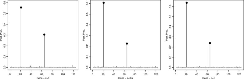
Lung cancer data: Marginal posterior probabilities for gene selection, p(θ_k|T, Y), for π = 0 (left), π = 0.5 (center) and π = 1 (right).

Figure 6.

Lung cancer data: Conditional posterior probabilities for SNP selection, p(γ_j|T, Y, I{Σ_k θ_ks_kj = 1}), for π = 0 (left), π = 0.5 (center) and π = 1 (right).

Our findings match those of other studies in the epidemiologic literature. SNP 754 in gene 21 refers to rs1051730 in CHRNA3 on chromosome 15, and SNP 747 in gene 65 refers to rs8034191 in AGPHPD1. Both SNPs have been found consistently associated with lung cancer risk and survival [2, 3, 23, 43, 44, 55, 57] and in strong LD with each other (R² = 0.85). CHRNA3 encodes the α–3 subunit of the nicotinic cholinergic receptor, which mediates cholinergic activity. Its polymorphisms have been shown to affect both lung cancer risk and smoking behaviors [25, 53]. Rs8034191 is in the intronic region of AGHPD1. Although SNPs in this locus have been known for some time, the actual function of AGHPD1 is yet to be uncovered [52] and therefore the biological role of AGHPD1 in lung cancer is still under investigation.

For comparison, we analyzed the lung cancer data with the method proposed by [19]. SNP 754 was the only SNP identified by this approach, with a posterior probability of 0.62. This approach assigned to SNP 747 a posterior probability of being related to the disease of 0.25.

4. DISCUSSION

We have proposed a novel Bayesian modeling construction to identify molecular biomarkers for disease prediction in genome-wide association studies. We have defined gene-level scores based on SNP genotypes and used a linear modeling setting to study their association to the observed phenotype. In our gene-level scores the observed SNP frequencies are weighted using the population frequencies as defined by the Hardy-Weinberg equilibrium law, giving more importance to the unusually low frequencies, i.e. to the SNPs that might indicate peculiar genetic differences between subjects belonging to different groups. An additional feature of our model is the incorporation of information on SNP-to-SNP associations via network priors that capture non-random associations between pairs of SNPs based on their linkage disequilibrium. For posterior inference we have designed a stochastic search method that identifies significant biomarkers (SNPs and genes) for disease prediction. Our method has shown good performances on simulated data and on a lung cancer dataset. Overall, our results have suggested that including biological information in the model helps achieve a sharper selection, particularly in situations where the number of causal SNPs is extremely small with respect to the number of non predictive (noisy) SNPs.

In defining our gene-level scores we have followed other authors, in particular those of [27], who proposed a similarity measure between groups of subjects genotyped for numerous genetic loci which is based on weighing the genetic profiles according to the estimates of gene frequencies at Hardy-Weinberg equilibrium in the population. Other scoring methods may be designed. [8] considers several data-driven measures proposed in the literature to capture similarity between two categorical data instances. The authors evaluate performances of the methods in the context of a specific data mining task, that is outlier detection. They conclude that, while no one measure dominates the others for all types of problems, some measures have consistently high performance.

A common problem in variable selection is how to define a best cut-off on the marginal posterior probabilities of inclusion, for posterior inference. Several alternative approaches are commonly used, such as the median probability model (i.e. threshold of 0.5) of [4] and the expected FDR of [32], just to name a couple. On the other hand, a threshold is not always needed as the posterior probabilities naturally rank the variables (genes and SNPs in our case) and can be used to prioritize the findings that, in real studies, will need to be eventually validated. We have used a threshold of 0.5 for comparison and, in addition, commented on genes and SNPs with non-negligible posterior probabilities (lower than 0.5) as a way to provide investigators additional findings that can be possibly validated.

In the construction of our model we have incorporated external biological information, in particular using network priors that capture non-random associations between pairs of SNPs based on their linkage disequilibrium. Additional information is available on gene-to-gene regulatory networks, for example via the KEGG database, and could be incorporated into the model via the prior (7) on the parameter θ_k. Also, although we have not done this here, our method can be easily extended to handle SNPs that belong to more than one gene, in case of overlapping genes, by adding constraints to our MCMC algorithm [47]. For SNPs in a “desert” region, far away from any gene, our method is flexible enough to group these SNPs together as their own group/covariate.

We have demonstrated that our method is suitable for analyzing SNPs that have minor allele frequencies greater than 5% in a candidate region, as a follow up to a genome-wide association study. In particular, the method has been shown to work for scenarios with p ≫ n. In theory, our method can be applied to any such scenario, including whole genome-wide scenarios. However, as it is computationally intense, some dimensionality reduction would be needed, for example one could apply the sure independence screening of [15] to reduce the number of SNPs to a level that is computationally feasible. As some SNPs are excluded from the analysis in the pre-selection step, our model estimates marginal effects with respect to the excluded SNPs. The pre-selection step does not depend on the data, but is determined based on some biological considerations on specific areas of interest of the DNA, and therefore does not introduce any selection bias.

Finally, our method can also be applied to rare variants, although it would need computational adjustments. In particular, for rare variants, i.e., minor allele frequencies less than 1%, the detection of individual rare variants may be challenging without proper adjustments that go beyond the scope of the application here presented.

APPENDIX. DETAILS OF THE MCMC ALGORITHM

Our MCMC scheme consists of two steps:

• This step updates (θ, γ) by adding or deleting one gene and/or one SNP as follows:

  1. Change the inclusion status of both gene and SNP -randomly choose between addition or removal.

     • (1.i)
       Add a gene and a SNP:

       • First select a gene that is not included in the model then randomly choose one SNP from the gene $({\gamma }_j^{\mathit{old}}=0)$ and propose including both the gene and the SNP, i.e., set ${\theta }_k^{\mathit{new}}=1$, ${\gamma }_j^{\mathit{new}}=1$. The move is accepted with probability min(1, α) with

         $$\alpha =\frac{f({\theta }^{\mathit{new}},{\gamma }^{\mathit{new}}|T,Y)}{f({\theta }^{\mathit{old}},{\gamma }^{\mathit{old}}|T,Y)}\cdot \frac{\mathit{pk}\cdot {\displaystyle {\sum }_{r=1}^{K}I\{{\theta }_r^{\mathit{old}}=0,p_{r\gamma }^{\mathit{old}}=0\}}}{{\displaystyle {\sum }_{r=1}^{K}I\{{\theta }_r^{\mathit{new}}=1,p_{r\gamma }^{\mathit{new}}=1\}}}.$$
     • (1.ii)
       Remove a gene and a SNP:

       • This move is the reverse of (1.i) described above. First select a gene that is included in the model that has only one of its member SNPs included in the model $({\theta }_k^{\mathit{old}}=1\text{and}{p}_{k\gamma }^{\mathit{old}}=1)$. Attempt to remove both the gene and the SNP, i.e., set ${\theta }_k^{\mathit{new}}=0$, ${\gamma }_j^{\mathit{new}}=0$ and accept the move with probability min(1, α) with

         $$\alpha =\frac{f({\theta }^{\mathit{new}},{\gamma }^{\mathit{new}}|T,Y)}{f({\theta }^{\mathit{old}},{\gamma }^{\mathit{old}}|T,Y)}\cdot \frac{{\displaystyle {\sum }_{r=1}^{K}I\{{\theta }_r^{\mathit{old}}=1,p_{r\gamma }^{\mathit{old}}=1\}}}{\mathit{pk}\cdot {\displaystyle {\sum }_{r=1}^{K}I\{{\theta }_r^{\mathit{new}}=0,p_{r\gamma }^{\mathit{new}}=0\}}}.$$
  2. Change the inclusion status of a SNP but not the gene – randomly choose between addition (2.i) or removal (2.ii).

     • (2.i)
       Add a SNP in an already included gene:

       • First select a gene already included in the model and that has some member SNPs that could potentially be added $({\theta }_k^{\mathit{old}}=1\text{and}\mathit{pk}>p_{k\gamma }^{\mathit{old}})$. Let G be the set of genes that satisfy these conditions. Choose one of the non-included SNPs from this gene $({\gamma }_j^{\mathit{old}}=0)$ and attempt to add it, i.e, set ${\theta }_k^{\mathit{new}}={\theta }_k^{\mathit{old}}=1$, γ^new = 1. The proposal is accepted with probability min(1, α) with

         $$\begin{array}{l}\alpha =\frac{f({\theta }^{\mathit{new}},{\gamma }^{\mathit{new}}|T,Y)}{f({\theta }^{\mathit{old}},{\gamma }^{\mathit{old}}|T,Y)}\cdot \frac{{\displaystyle {\sum }_{r=1}^{K}I\{{\theta }_r^{\mathit{old}}=1,p_r>p_{r\gamma }^{\mathit{old}}\}}}{{\displaystyle {\sum }_{r=1}^{K}I\{{\theta }_r^{\mathit{new}}=1,p_{r\gamma }^{\mathit{new}}>1\}}}\\ \frac{{\displaystyle {\sum }_{r\in G}\frac{1}{p_{r\gamma }^{\mathit{new}}}}}{{\displaystyle {\sum }_{r\in G}\frac{1}{\mathit{Pr}-p_{r\gamma }^{\mathit{old}}}}}.\end{array}$$
     • (2.ii)
       Remove a SNP from an already included gene:

       • This move is the reverse of (2.i) described above. First select a gene already included in the model that has more than one of its member SNPs included in the model $({\theta }_k^{\mathit{old}}=1,p_{k\gamma }^{\mathit{old}}>1)$. Once the gene is selected, choose a SNP among the eligible candidates, that is, an included SNP $({\gamma }_j^{\mathit{old}}=1)$. Leave the gene status unchanged and attempt to remove the selected SNP, i.e., set ${\theta }_k^{\mathit{new}}={\theta }_k^{\mathit{old}}=1$, ${\gamma }_j^{\mathit{new}}=0$. The proposed move is accepted with probability min(1, α) with

         $$\begin{array}{l}\alpha =\frac{f({\theta }^{\mathit{new}},{\gamma }^{\mathit{new}}|T,Y)}{f({\theta }^{\mathit{old}},{\gamma }^{\mathit{old}}|T,Y)}\cdot \frac{{\displaystyle {\sum }_{r=1}^{K}I\{{\theta }_r^{\mathit{old}}=1,p_{r\gamma }^{\mathit{old}}>1\}}}{{\displaystyle {\sum }_{r=1}^{K}I\{{\theta }_r^{\mathit{new}}=1,p_r>p_{r\gamma }^{\mathit{new}}\}}}\\ \frac{{\displaystyle {\sum }_{r\in G}\frac{1}{p_r-p_{r\gamma }^{\mathit{new}}}}}{{\displaystyle {\sum }_{r\in G}\frac{1}{p_{r\gamma }^{\mathit{old}}}}}.\end{array}$$
     For interpretability, as previously described, no empty genes or orphan SNPs are proposed during sampling.
• In this step the latent variables z_is are sampled from truncated normal distributions under the constraint defined by equation (2). As the sample size is often large in genetic association studies, we found it more convenient to sample from the full conditional of each z_i given all the other z_j’s (j ≠ i) and (γ, θ), rather than sample the entire vector Z from a multivariate truncated normal distribution:

  $$z_i|z_j,y_i,\gamma ,\theta =\{\begin{array}{ll}N(m_i,v_i)I(z_i>0)\hfill & \text{if}{y}_i=1\hfill \\ N(m_i,v_i)I(z_i<0)\hfill & \text{if}{y}_i=0\hfill \end{array}$$

  where m_i and v_i can be efficiently calculated following [22].

References

- 1.Albert J, Chib S. Bayesian analysis of binary and polychotomous response data. Journal of American Statistical Association. 1993;88:669–679. MR1224394. [Google Scholar]
- 2.Amos C, Wu X, Broderick P, Gorlov I, Gu J, Eisen T, Dong Q, Zhang Q, Gu X, Vijayakrishnan J, Sullivan K, Matakidou A, Wang Y, Mills G, Doheny K, Tsai Y, Chen W, Shete S, Spitz M, Houlston R. Genome-wide association scan of tag SNPs identifies a susceptibility locus for lung cancer at 15q25.1. Nature Genetics. 2008;40(5):616–622. doi: 10.1038/ng.109. [DOI] [PMC free article] [PubMed] [Google Scholar]
- 3.Amos C, Gorlov I, Dong Q, Wu X, Zhang H, Lu E, Scheet P, Greisinger A, Mills G, Spitz M. Nicotinic acetylcholine receptor region on chromosome 15q25 and lung cancer risk among African Americans: a case-control study. Journal of the National Cancer Instute. 2010;102:1199–1205. doi: 10.1093/jnci/djq232. [DOI] [PMC free article] [PubMed] [Google Scholar]
- 4.Barbieri M, Berger J. Optimal predictive model selection. Ann Stat. 2004;32(3):870–897. MR2065192. [Google Scholar]
- 5.Barrett J, Fry B, Maller J, Daly M. Haploview: analysis and visualization of LD and haplotype maps. Bioinformatics. 2005:263–265. doi: 10.1093/bioinformatics/bth457. [DOI] [PubMed] [Google Scholar]
- 6.Besag J. Spatial interaction and the statistical analysis of lattice systems. Journal of the Royal Statistical Society, Ser B. 1974;36:192–225. MR0373208. [Google Scholar]
- 7.Bigdeli T, Maher B, Zhao Z, Sun J, Medeiros H, Akula N, McMahon F, Carvalho C, Ferreira S, Azevedo M, Knowles J, Pato M, Pato C, Fanous A. Association study of 83 candidate genes for bipolar disorder in chromosome 6q selected using an evidence-based prioritization algorithm. Am J Med Genet B Neuropsychiatr Genet. 2013;162(8):898–906. doi: 10.1002/ajmg.b.32200. [DOI] [PubMed] [Google Scholar]
- 8.Boriah S, Chandola V, Kumar V. Similarity measures for categorical data: A comparative evaluation. SIAM Data Mining Conference. 2008:243–254. [Google Scholar]
- 9.Chen L, Hutter C, Potter J, Liu Y, Prentice R, Peters U, Hsu L. Insights into colon cancer etiology via a regularized approach to gene set analysis of GWAS data. Am J Hum Genet. 2010a;86:860–871. doi: 10.1016/j.ajhg.2010.04.014. [DOI] [PMC free article] [PubMed] [Google Scholar]
- 10.Chen X, Wang L, Hu B, Guo M, Barnard J, Zhu X. Pathway-based analysis for genome-wide association studies using supervised principal components. Genetic Epidemiology. 2010b;34(7):716–724. doi: 10.1002/gepi.20532. [DOI] [PMC free article] [PubMed] [Google Scholar]
- 11.Conti D, Gauderman W. SNPs, haplotypes, and model selection in a candidate gene region: the simple analysis for multilocus data. Genetic Epidemiology. 2004;27(4):429–41. doi: 10.1002/gepi.20039. [DOI] [PubMed] [Google Scholar]
- 12.Cox D. On an internal method for deriving a summary measure. Biometrika. 2008;95(4):1002–1005. MR2461228. [Google Scholar]
- 13.Dickson S, Wang K, Krantz I, Hakonarson J, Goldstein D. Rare variants create synthetic genome-wide associations. PLoS Biology. 2010;8:e1000294. doi: 10.1371/journal.pbio.1000294. [DOI] [PMC free article] [PubMed] [Google Scholar]
- 14.Eichler E, Flint J, Gibson G, Kong A, Leal S, Moore J, Nadeau J. Missing heritability and strategies for finding the underlying causes of complex disease. Nature Reviews Genetics. 2010;11:446–450. doi: 10.1038/nrg2809. [DOI] [PMC free article] [PubMed] [Google Scholar]
- 15.Fan J, Song R. Sure independence screening in generalized linear models with np-dimensionality. The Annals of Statistics. 2010;38(6):3567–3604. MR2766861. [Google Scholar]
- 16.Fridley. Bayesian variable and model selection method for genetic associaton studies. Genet Epi. 2009;33:27–37. doi: 10.1002/gepi.20353. [DOI] [PubMed] [Google Scholar]
- 17.George EI, McCulloch RE. Approaches for Bayesian variable selection. Statistica Sinica. 1997;7:339–373. [Google Scholar]
- 18.Gibson G. Rare and common variants: twenty arguments. Nature Reviews Genetics. 2011;13:135–145. doi: 10.1038/nrg3118. [DOI] [PMC free article] [PubMed] [Google Scholar]
- 19.Guan Y, Stephens M. Bayesian variable selection regression for genome-wide association studies, and other large-scale problems. Annals of Applied Statistics. 2011;5(3):1780–1815. MR2884922. [Google Scholar]
- 20.Han F, Pan W. A composite likelihood approach to latent multivariate Gaussian modeling of SNP data with application to genetic association testing. Biometrics. 2012;68(1):307–15. doi: 10.1111/j.1541-0420.2011.01649.x. MR2909887. [DOI] [PMC free article] [PubMed] [Google Scholar]
- 21.Hartl DL, Clark A. Principles of population genetics. 3 Sinauer Associates; Sunderland, MA: 1997. [Google Scholar]
- 22.Henderson H, Searle S. On deriving the inverse of a sum of matrices. SIAM Review. 1981;23(1):53–60. MR0605440. [Google Scholar]
- 23.Hung R, Mckay J, Gaborieau V, Boffetta P, Hashibe M, Zadridze D, Mukeria A, Szeszenia-Dabrowska N, Lissowska J, Rudnai P, Fabianova E, Mates D, Bencko V, Foretova L, Janout V, Chen C, Goodman G, Field J, Liloglou T, xinarianos G, Cassidy A, McLaughlin J, Liu G, Narod S, Krokan H, Skorpen F, Elvestad MB, Hveem K, Vatten L, Linseisen J, Clavel-Chapelon F, Vineis P, Bueno-de Mesquita H, Lund E, Martinez C, Bingham S, Rasmuson T, Hainaut P, Riboli E, Ahrens W, Benhamou S, Lagiou P, Trichopoulos D, Holcatova I, Merletti F, Kjaerheim K, Aguidos A, Macfarlane G, Talamini R, Simonato L, Lowery R, Conway D, Znaor A, Healy C, Zelenika D, Boland A, Delepine M, Foglio M, Lechner D, Matsuda F, Blanceh H, Gut I, Heath S, Lat Hrop M, Brennan P. A susceptibility locus for lung cancer maps to nicotinic acetylcholine receptor subunit genes on 15q25. Nature. 2008;452:633–637. doi: 10.1038/nature06885. [DOI] [PubMed] [Google Scholar]
- 24.Kääb S, Crawford D, Sinner M, Behr E, Kannankeril P, Wilde A, Bezzina C, Schulze-Bahr E, Guicheney P, Bishopric N, Myerburg R, Schott J, Pfeufer A, Beckmann B, Martens E, Zhang T, Stallmeyer B, Zumhagen S, Denjoy I, Bardai A, Van Gelder I, Jamshidi Y, Dalageorgou C, Marshall V, Jeffery S, Shakir S, Camm A, Steinbeck G, Perz S, Lichtner P, Meitinger T, Peters A, Wichmann H, Ingram C, Bradford Y, Carter S, Norris K, Ritchie M, George A, Roden D. A large candidate gene survey identifies the KCNE1 D85N polymorphism as a possible modulator of drug-induced torsades de pointes. Circ Cardiovasc Genet. 2012;5(1):91–9. doi: 10.1161/CIRCGENETICS.111.960930. [DOI] [PMC free article] [PubMed] [Google Scholar]
- 25.Kaur-Knudsen D, Bojesen S, Tybjaerg-Hansen A, Nordestgarrd B. Nicotinic acetylcholine receptor polymorphism, smoking behavior, and tobacco-related cancer and lung and cardiovascular diseases: a cohort study. Journal of Clinical Oncology. 2011;29:2875–2882. doi: 10.1200/JCO.2010.32.9870. [DOI] [PubMed] [Google Scholar]
- 26.Kwon D, Tadesse M, Sha N, Pfeiffer R, Vannucci M. Identifying biomarkers from mass spectrometry data with ordinal outcome. Cancer Informatics. 2007;3:19–28. [PMC free article] [PubMed] [Google Scholar]
- 27.Lagani V, Montesanto A, Di Cianni F, Moreno V, Landi S, Conforti D, Rose G, Passarino G. A novel similarity-measure for the analysis of genetic data in complex phenotypes. BMC Bioinformatics. 2009;10(Suppl 6):S24. doi: 10.1186/1471-2105-10-S6-S24. [DOI] [PMC free article] [PubMed] [Google Scholar]
- 28.Li F, Zhang N. Bayesian Variable Selection in Structured High-Dimensional Covariate Space with Application in Genomics. Journal of American Statistical Association. 2010;105:1202–1214. MR2752615. [Google Scholar]
- 29.Li H, Wei Z, Maris J. A hidden Markov random field model for genome-wide association studies. Biostatistics. 2010;11(1):139–150. doi: 10.1093/biostatistics/kxp043. [DOI] [PMC free article] [PubMed] [Google Scholar]
- 30.Madsen B, Browning S. A groupwise association test for rare mutations using a weighted sum statistic. PLoS Genetics. 2009;5(2):e1000384. doi: 10.1371/journal.pgen.1000384. [DOI] [PMC free article] [PubMed] [Google Scholar]
- 31.Manolio T, Collins F, Cox N, Goldstein D, Hindorff L, Hunter D, McCarthy M, Ramos E, Cardon L, Chakravarti A, Cho J, AE G, Kong A, Kruglyak L, Mardis E, Rotimi C, Slatkin M, Valle D, Wittmore A, Boehnke M, Clark A, Eichler E, Gibson G, Haines J, Mackay T, McCarroll S, Visscher P. Finding the missing heritability of complex diseases. Nature. 2009;461:747–753. doi: 10.1038/nature08494. [DOI] [PMC free article] [PubMed] [Google Scholar]
- 32.Newton M, Noueiry A, Sarkar D, Ahlquist P. Detecting differential gene expression with a semiparametric hierarchical mixture method. Biostatistics. 2004;5(2):155–176. doi: 10.1093/biostatistics/5.2.155. [DOI] [PubMed] [Google Scholar]
- 33.Pan W. A unified framework for detecting genetic association with multiple SNPs in a candidate gene or region: contrasting genotype scores and LD patterns between cases and controls. Hum Hered. 2010;69(1):1–13. doi: 10.1159/000243149. [DOI] [PMC free article] [PubMed] [Google Scholar]
- 34.Peng B, Kimmel M. simupop: a forward-time population genetics simulation environment. Bioinformatics. 2005;21:3686–3687. doi: 10.1093/bioinformatics/bti584. [DOI] [PubMed] [Google Scholar]
- 35.Peng B, Amos CI, Kimmel M. Forward-time simulations of human populations with complex diseases. PLoS Genetics. 2007;3:e47. doi: 10.1371/journal.pgen.0030047. [DOI] [PMC free article] [PubMed] [Google Scholar]
- 36.Propp J, Wilson D. Exact sampling with coupled Markov chains and applications to statistical mechanics. Random Structures and Algorithms. 1996;9(1):223–252. MR1611693. [Google Scholar]
- 37.Purcell S, Neale B, Todd-Brown K, Thomas L, Ferreira M, Bender D, Maller J, Sklarb P, de Bakkerb P, Dalyb M, Sham P. Plink: A tool set for whole-genome association and population-based linkage analyses. The American Journal of Human Genetics. 2007;81(3):559–575. doi: 10.1086/519795. [DOI] [PMC free article] [PubMed] [Google Scholar]
- 38.Quintana M, Berstein J, Thomas D, Conti D. Incorporating model uncertainty in detecting rare variants: The Bayesian risk index. Genet Epi. 2011;35:638–649. doi: 10.1002/gepi.20613. [DOI] [PMC free article] [PubMed] [Google Scholar]
- 39.Schwender H, Ruczinski I, Ickstadt K. Testing SNPs and sets of SNPs for importance in association studies. Biostatistics. 2011;12:18–32. doi: 10.1093/biostatistics/kxq042. [DOI] [PMC free article] [PubMed] [Google Scholar]
- 40.Sha N, Vannucci M, Tadesse MG, Brown PJ, Dragoni I, Davies N, Roberts TC, Contestabile A, Salmon N, Buckley C, Falciani F. Bayesian variable selection in multinomial probit models to identify molecular signatures of disease stage. Biometrics. 2004;60:812–819. doi: 10.1111/j.0006-341X.2004.00233.x. MR2089459. [DOI] [PubMed] [Google Scholar]
- 41.Shahbaba B, Shachaf C, Yu Z. A pathway analysis method for genome-wide association studies. Statistics in Medicine. 2012;31(10):988–1000. doi: 10.1002/sim.4477. MR2913874. [DOI] [PubMed] [Google Scholar]
- 42.Sham P. Statistics in human genetics. Arnold; London: 1997. [Google Scholar]
- 43.Shiraishi K, Kohno T, Kunitoh H, Watanabe S, Goto K, Nishiwaki Y, Shimada Y, Hirose H, Saito I, Kuchiba A, Yamamoto S, Yokota A. Contribution of nicotine acetylcholine receptor polymorphisms to lung cancer risk in a smoking independent manner in the japanese. Carcinogenesis. 2009;30:65–70. doi: 10.1093/carcin/bgn257. [DOI] [PubMed] [Google Scholar]
- 44.Spitz M, CI A, Dong Q, Lin J, Wu X. The CHRNA5-A3 region on chromosome 15q24-25.1 is a risk factor both for nicotine dependence and for lung cancer. Journal of the National Cancer Institute. 2008;100:1552–1556. doi: 10.1093/jnci/djn363. [DOI] [PMC free article] [PubMed] [Google Scholar]
- 45.Srivastava S, Chen L. Comparison between the stochastic search varriable selection and the least absolute shrinkage and selection operator for genome-wide association studies in rheumatoid arthritis. BMC Proc. 2009;3(7):S21. doi: 10.1186/1753-6561-3-s7-s21. [DOI] [PMC free article] [PubMed] [Google Scholar]
- 46.Stephens M, Balding S. Bayesian statistical methods for genetic association studies. Nat Rev Genet. 2009;10:681–690. doi: 10.1038/nrg2615. [DOI] [PubMed] [Google Scholar]
- 47.Stingo F, Chen Y, Tadesse M, Vannucci M. Incorporating biological information into linear models: A Bayesian approach to the selection of pathways and genes. Annals of Applied Statistics. 2011;5(3):1978–2002. doi: 10.1214/11-AOAS463. MR2884929. [DOI] [PMC free article] [PubMed] [Google Scholar]
- 48.Swartz M, Shete S. The null distribution of stochatic search gene suggestion: A Bayesian approach to gene mapping. BMC Proceedings I. 2007;(suppl 1):S113. doi: 10.1186/1753-6561-1-s1-s113. [DOI] [PMC free article] [PubMed] [Google Scholar]
- 49.Swartz M, Kimmel M, Mueller P, Amos C. Stochastic search gene suggestion: A Bayesian hierarchical model for gene mapping. Biometrics. 2006;62(2):495–503. doi: 10.1111/j.1541-0420.2005.00451.x. MR2236832. [DOI] [PubMed] [Google Scholar]
- 50.Swartz M, Yu R, Shete S. Finding factors influencing risk: Comparing Bayesian stochastic search and standard variable selection methods applied to logistic regression models of cases and controls. Stat Med. 2008;27(6):6158–6174. doi: 10.1002/sim.3434. MR2522315. [DOI] [PMC free article] [PubMed] [Google Scholar]
- 51.Swartz M, Peterson C, Lupo P, Wu X, Forman M, Spitz M, Hernandez L, Vannucci M, Shete S. Investigating multiple candidate genes and nutrients in the folate metabolism pathway to detect genetic and nutritional risk factors for lung cancer. PLoS One. 2013;8(1):e53475. doi: 10.1371/journal.pone.0053475. [DOI] [PMC free article] [PubMed] [Google Scholar]
- 52.Veiga-da Cunha M, Hadi F, Ballingand T, Stroobant V, Van Schaftingen E. Molecular identification of hydroxylysine kinase and of ammonioph-spholyases actingon 5-phosphohydroxy-l-lysine and phosphoethanolamine. Journal of Biological Chemistry. 2012;287:7246–7255. doi: 10.1074/jbc.M111.323485. [DOI] [PMC free article] [PubMed] [Google Scholar]
- 53.Wassenaar C, Dong Q, Wei Q, Amos C, Spiz M, Tyndale R. Relationship between cyp2a6 and chrna5-chrna3-chrnb4 variation and smoking behaviors and lung cancer risk. Journal of the National Cancer Institue. 2011;103:1342–1346. doi: 10.1093/jnci/djr237. [DOI] [PMC free article] [PubMed] [Google Scholar]
- 54.Watanabe S. Asymptotic equivalence of Bayes cross validation and widely applicable information criterion in singular learning theory. Journal of Machine Learning Research. 2010;11:3571–3594. MR2756194. [Google Scholar]
- 55.Wei C, H Y, Spitz M, Wu X, Chancoco H, Akiva P, Rechavi G, Brand H, Wun I, Frazier M, Amos C. A case control study of a sex specific association between a 15q25 variant and lung cancer risk. Cancer Epidemiology, Biomarkers, and Prevention. 2011;20:2603–2609. doi: 10.1158/1055-9965.EPI-11-0749. [DOI] [PMC free article] [PubMed] [Google Scholar]
- 56.Wei Z, Li H. A hidden spatial-temporal markov random field model for network-based analysis of time course gene expression data. Annals of Applied Statistics. 2008;2(1):408–429. MR2415609. [Google Scholar]
- 57.Xun W, Brennan P, Tjonneland A, Vogel U, Overvad K, Kaaks R, Canzian F, Boeing H, Trichopoulou A, Oustoglou E, Giotaki Z, Johansson M, Palli D, Agnoli C, Turmino R, Sacerdote C, Panico S, Bueno-de Mesquita H, Peeters P, Lund E, Kumle M, Rodriguez L, Agudo A, Sanchez M, Arriola L, Chirlaque M, Barricarte A, Hallmans G, Rasmuson T, Khaw K, Wareham N, Key T, Riboli E, Vineis P. Single-nucleotide polymorphisms (5p15.33, 15q25.1, 6p22.1, 6q27 and 7p15.3) and lung cancer survival in the European prospective investigation into cancer and nutrition (EPIC) Mutagenesis. 2011;26:657–666. doi: 10.1093/mutage/ger030. [DOI] [PubMed] [Google Scholar]
- 58.Yi N, Zhi D. Bayesian analysis of rare variants in genetic association studies. Genet Epi. 2011;35:57–69. doi: 10.1002/gepi.20554. [DOI] [PMC free article] [PubMed] [Google Scholar]
- 59.Yi N, Kaklamani V, Pasche B. Bayesian analysis of genetic interactions in case-control studies, with application to adiponectin genes and colorectal cancer risk. Annals of Human Genetics. 2011;75(1):90–104. doi: 10.1111/j.1469-1809.2010.00605.x. [DOI] [PMC free article] [PubMed] [Google Scholar]
- 60.Zuk O, Hechter E, Sunyaev S, Lander E. The mystery of missing heritability: Genetic interactions create phantom heritability. Proceedings of the National Academy of Science USA. 2012;109(4):1193–1198. doi: 10.1073/pnas.1119675109. [DOI] [PMC free article] [PubMed] [Google Scholar]