Learning-Based Structurally-Guided Construction of Resting-State Functional Correlation Tensors

Abstract

Functional magnetic resonance imaging (fMRI) measures changes in blood-oxygenation-level-dependent (BOLD) signals to detect brain activities. It has been recently reported that the spatial correlation patterns of resting-state BOLD signals in the white matter (WM) also give WM information often measured by diffusion tensor imaging (DTI). These correlation patterns can be captured using functional correlation tensor (FCT), which is analogous to the diffusion tensor (DT) obtained from DTI. In this paper, we propose a noise-robust FCT method aiming at further improving its quality, and making it eligible for further neuroscience study. The novel FCT estimation method consists of three major steps: First, we estimate the initial FCT using a patch-based approach for BOLD signal correlation to improve the noise robustness. Second, by utilizing the relationship between functional and diffusion data, we employ a regression forest model to learn the mapping between the initial FCTs and the corresponding DTs using the training data. The learned forest can then be applied to predict the DTI-like tensors given the initial FCTs from the testing fMRI data. Third, we re-estimate the enhanced FCT by utilizing the DTI-like tensors as a feedback guidance to further improve FCT computation. We have demonstrated the utility of our enhanced FCTs in Alzheimer’s disease (AD) diagnosis by identifying mild cognitive impairment (MCI) patients from normal subjects.

1 Introduction

Functional magnetic resonance imaging (fMRI) has emerged as the primary non-invasive technique for measuring neural activity in the brain. Since the introduction of fMRI in the early 1990s, it has been widely used for its sensitivity to developmental, aging and pathological processes of various organs [1]. fMRI is designed to detect hemodynamic changes in the gray matter (GM) regions, which are known to be associated with the neural activity [2]. An increase of the neural activation usually causes increased local cerebral blood flow to supply the metabolic demands [3]. The measurement of such variation is called blood-oxygenation-level-dependent (BOLD) time series.

Extensions of fMRI have been proposed for the needs in different clinical and research fields. For example, task-based fMRI [4] was developed to localize functionally specialized brain regions under specific task stimulus. On the other hand, the resting-state fMRI (rs-fMRI) [5] is collected in a task-free state and has usually been applied to discover correlated activity patterns or functional connectivity (FC) among different brain regions, in an either local or distant manner. However, in contrast to the GM regions, it is much harder to detect the BOLD signals in the brain white matter (WM), as WM is irrigated by much less dense vasculature [6] and the blood flow in WM is approximately one-fourth of that in GM [7].

Diffusion tensor imaging (DTI), or more generally, the diffusion-weighted magnetic resonance imaging (DWI), has been recognized as an effective tool in the study of the WM [8]. DTI quantifies the diffusion patterns of water molecules using a diffusion tensor (DT) represented by a 3×3 symmetric matrix. The movement of water molecules is less constrained in the axonal direction than the perpendicular directions. Thus, using a diffusion tensor model, the distribution of movement of water molecules can be simply represented by an ellipsoid, with the axonal direction given by the major axis. Various diffusion parameters, such as fractional anisotropy (FA), mean diffusivity (MD), axial diffusivity (AD) and radial diffusivity (RD), can be calculated based on the DTs. These parameters have been used extensively for WM abnormality detection for various neurological and psychiatric diseases [9]. Furthermore, the directions of the DTs can be further employed using diffusion tractography to map WM fiber pathways [10], complementary to the GM connectivity information given by FC networks [11].

fMRI has also been used to investigate connectivity in WM. For instance, it was found in [12] that fMRI activation can also be observed in the genu of the corpus callosum. This finding was confirmed by D’Arcy et al. [13] using a Sperry task. Activation in the splenium of the corpus callosum was also observed, providing the first fMRI evidence of posterior callosal activation associated with an interhemispheric transfer task. The work in Mazerolle et al. [14] expanded and refined the approach taken by D’Arcy et al. [13]. Outside of the corpus callosum, BOLD fMRI activation has also been reported, such as in the internal capsule. For example, Mosier and colleagues reported activation associated with swallowing in the internal capsule, as well as the corpus callosum [15]. Also, Gawryluk et al. [16] found that activation can be detected in the internal capsule during a motor task (i.e., finger tapping), which was later confirmed by Mazerolle et al. in [17]. These findings indicate that the BOLD fMRI signals potentially exist in the WM regions due to the existence and detectability of the vasculature, cerebral blood flow (CBF), and cerebral blood volume (CBV) in the WM [18]. Marussich et al. [19] also investigated spatiotemporal correlation of BOLD fMRI signals in WM, comparing between eye-closed resting state and visual-perception tasks. They showed WM functional connectivity in the resting-state session, as well as significant correlations between optical radiations and multiple cortical visual networks.

Recently, Ding et al. [20] found the weak but putative local temporal correlation of BOLD signals that persists over a long distance along the same WM neuronal fiber tracts using rs-fMRI. This study found functional anisotropy of local FCs between a central WM voxel and its neighboring voxels. They captured this anisotropy using a local spatiotemporal correlation tensor and demonstrated that the realistic fiber bundle can be obtained by tracing the directions of FCs. They subsequently introduced “functional correlation tensor (FCT)” in [21] and demonstrated the ability of FCT in revealing several major WM fiber bundles, indicating that FCT is coherent with DTI. However, our experiments indicate that FCTs are sensitive to noise. Since there is only 1–3% signal variability associated with the BOLD signal in GM [22], while it is much less in WM [23], computing FC in WM is challenging.

To address the aforementioned issues, here we propose a novel framework for further improving FCT estimation with the guidance of DT information. The aim is to reduce the influence of noise in WM to the FCT estimation, which is referred from the finding of the consistency between the WM fiber direction and the spatiotemporal correlation pattern of the WM BOLD signals [20, 21]. The main contribution in this paper is four-fold: First, we develop a novel strategy, aiming at increasing the noise robustness of FCT using a patch-based approach. Second, to cater to the possibility that only rs-fMRI but not DTI data are available, we intend to predict DTI-like tensors from the computed FCTs. Specifically, we incorporate the regression forest method to train the learning-based model, which has been successfully applied in many medical image analysis domains, such as image segmentation [24–26] and reconstruction [27]. We further adopt the cascaded learning strategy using the auto-context model introduced in [28] to boost the performance. Third, we further refine the estimation of FCTs by weighting the dominant directions on the basis of DTI-like tensors. Finally, we have demonstrated the utility of the enhanced FCT in early-stage mild cognitive impairment (eMCI) diagnosis.

2 Materials and Methods

In this section, we first illustrate the details of two datasets employed in our works, which are the development and the validation datasets. The development dataset is the Human Connectome Project (HCP)¹ [29], which contains high-resolution brain images in both modalities of fMRI and DTI, which suits our needs in training the regressor. We also consider the validation dataset as the ADNI² [30] dataset, in which we apply the estimated enhanced FCTs to demonstrate the quality. Details of the two datasets along with their pre-processing steps are presented in Section 2.1.

We also present the methodology of our works in this section. The overall pipeline is illustrated in Figure 1, which has the following three major steps:

1. We employ a patch-based strategy to estimate the initial FCT, for the aim of noise robustness.

2. We then incorporate the random forest technique for predicting DTI-like tensors from FCTs.

3. We compute the orientation distribution functions (ODFs) from the learned DTI-like tensors and use its directional information to compute the enhanced FCTs.

Figure 1.

The overall pipeline of the proposed FCT calculation framework.

In the following, we first illustrate three major steps in Section 2.2, Section 2.3 and Section 2.4, respectively. Then, in Section 2.5 we show the process of utilizing the obtained FCTs in the early diagnosis of MCI.

2.1 Materials

HCP dataset

The HCP dataset was initialized by the Washington University-University of Minnesota Human Connectome Project Consortium. The aim is to construct cohesive framework by collecting massive images with the major MRI neuroimaging modalities to enable cross-subject comparisons and multi-model analysis of brain architecture, connectivity, and function. The volunteer subjects were drawn from a population of 1200 healthy adults in the age range of 22–35 years.

To reduce the computation cost, we randomly select images of rs-fMRI and DWI from 95 subjects of the HCP dataset. All HCP subjects were scanned on a customized Siemens Skyra 3T scanner with the same imaging parameters [31]: For fMRI, TR=720 ms, TE=33 ms, multiband factor=8, image matrix=104×90, 72 slices, 1200 volumes, and isotropic slice size=2×2×2 mm³; For DTI, TR=5500 ms, TE=89 ms, multiband factor=3, image matrix=145×174, 145 slices, slice thickness=1.25×1.25×1.25 mm³, and multiple b values=1000, 2000, 3000 s/mm², with 3-shell HARDI (High Angular Resolution Diffusion Imaging) and 270 non-colinear directions.

The first 30 frames in the rs-fMRI images were removed for magnetization equilibrium. We then used the first 600 frames (7 min 12 s data) of the remaining data to calculate FCTs to improve the computing speed while keeping adequate temporal samples to get robust FC for extracting FCTs. Experiments show that the FCT output using 600 frames is quite similar with that using the entire 1200 frames. The pre-processing protocol to the rs-fMRI data follows the HCP Pipeline¹, as detailed in [31], but are optimized based on our specific requirements:

• The DTs were computed using the dtifit tool in FSL [32]. We also computed the average b0 image for inter-modality registration between DTI and rs-fMRI.

• The DT images along with the b0 images were down-sampled to 2 mm isotropic resolution for consistency with the rs-fMRI data. Note that each subject’s DTI data was also registered to their own “anterior commissure to posterior commissure (AC-PC)” aligned T1-weighted high-resolution structural MRI data. Our algorithm does not rely on MNI space registration.

• Different from the conventional fMRI studies, there is no registration process for the rs-fMRI data. The FCT computation is performed in the subject native space, to avoid the possible registration error that disturbs the quality of FCT.

• Band-pass filtering (0.01 ≤ f ≤ 0.08Hz) was applied to the rs-fMRI data. No spatial smoothing was applied.

ADNI Dataset

The ADNI dataset was launched in 2003 aiming at measuring the progression of mild cognitive impairment (MCI) and early Alzheimer’s disease (AD). We use this dataset to demonstrate the quality of enhanced FCTs and their ability in differentiating eMCI and normal control (NC). We used the data of 39 eMCI subjects and 42 NCs, which were age- and gender-matched. All rs-fMRI images were obtained using 3T Philips Achieva scanner at different centers. The first 3 volumes of each subject were first discarded for magnetization equilibrium. Pre-processing was performed using SPM8¹, REST², and DPARSFA³ to reduce the effects of nuisance signals. The rigid-body transformation was used for head motion correction, and images with head motion larger than 2mm or 2 degrees were discarded. Band-pass filtering (0.01 ≤ f ≤ 0.08 Hz) was applied to avoid physiological noise and measurement errors. Head motion parameters (Friston24) were regressed out from the rs-fMRI data.

2.2 Initial FCT Estimation

According to Ding et al. in [21], the FCT T_i for the voxel V_i in the input rs-fMRI can be represented using a 3×3 symmetric matrix. The elements in T_i are written as follows:

$${\mathit{T}}_i=\left[\begin{array}{ccc}{T}_{xx}& T_{xy}& T_{xz}\\ T_{xy}& T_{yy}& T_{yz}\\ T_{xz}& T_{yz}& T_{zz}\end{array}\right].$$ (1)

In [21], T_i is obtained using the following steps:

1. The voxel V_i computes its Pearson’s linear correlation coefficient C_ij with its surrounding 26 voxels V_j by comparing their time courses. The equation is given as C_ij = f_corr(V_i, V_j), where f_corr is a function to compute the Pearson’s correlation coefficient of the time courses of V_i and V_j.

2. The unit vector n_ij = {n_ij,₁, n_ij,2, n_ij,₃} is obtained, representing the direction from V_i to V_j. The dyadic tensor D_ij is therefore written as:

   $${\mathit{D}}_{ij}=\left(\begin{array}{ccc}{n}_{ij,1}\cdot n_{ij,1}& n_{ij,1}\cdot n_{ij,2}& n_{ij,1}\cdot n_{ij,3}\\ n_{ij,2}\cdot n_{ij,1}& n_{ij,2}\cdot n_{ij,2}& n_{ij,2}\cdot n_{ij,3}\\ n_{ij,3}\cdot n_{ij,1}& n_{ij,3}\cdot n_{ij,2}& n_{ij,3}\cdot n_{ij,3}\end{array}\right);$$ (2)
3. The correlation tensor T_i is obtained by summing up all the dyadic tensors D_ij with their corresponding C_ij as the weight coefficients, which is given as:

   $${\mathit{T}}_i={\displaystyle \sum _j{C}_{ij}{\mathit{D}}_{ij}}.$$ (3)

One of the limitations of [21] is that correlation is computed only voxel-wise. Due to the limited signal-to-noise ratio (SNR) of the WM BOLD signals, FCT estimation can be adversely affected by noise. For greater robustness to noise, we introduce a patch-based method for correlation computation. In this strategy, the time series of not only one voxel, but also those from the neighboring voxels, are used to improve robustness to noise. Specifically, the patch-based strategy is presented as follows:

1. The number of surrounding voxels for V_i for FCT computation is no longer limited to 26. For a m × m ×m neighborhood window with V_i as its center voxel, the correlation coefficients are computed by traversing all voxels within the window. Note that the number of the surrounding voxels involved becomes m³ − 1 instead.

2. A novel patch-based strategy is used for correlation computation. Denote Q(x, y, z) to be the voxel at location (x, y, z) of the k × k × k patch Q. Inspired by Heinrich et al. [33], we first compute the voxel-wise correlation of the two patches, and then combine the correlations. For two patches Q_i and Q_j, the correlation coefficient C′_ij for the patch-based strategy is obtained by

   $$C_{ij}^{\prime }=\frac{{\sum }_{x=1}^k{\sum }_{y=1}^k{\sum }_{z=1}^{k}b(x,y,z)f_{\text{corr}}\left(Q_i(x,y,z),Q_j(x,y,z)\right)}{{\sum }_{x=1}^k{\sum }_{y=1}^k{\sum }_{z=1}^{k}b(x,y,z)},$$ (4)

   where b(x, y, z) is the Gaussian kernel given as $b(x,y,z)=\text{exp}(-\frac{{\left(x-\mu \right)}^2+{\left(y-\mu \right)}^2+{\left(z-\mu \right)}^2}{2{\rho }^2})$, μ = (k + 1)/2, and ρ is a scaling coefficient. Our experiments show that ρ² = 1.25 gives the optimal results.

Note that in the experiments we apply the same settings for both the HCP and the ADNI datasets: the patch size for the correlation measurement is 3×3×3 in voxel, and the neighborhood window size is 5×5×5 in voxel. The first step of the proposed framework can be summarized in Figure 2. Since FCT is represented by a symmetric matrix, it can be denoted here as a vector with 6 elements {T_xx, T_xy, T_xz, T_yy, T_yz, T_zz}.

Figure 2.

Initial FCT computation. For the voxel V_i in the brain region of the rs-fMRI data, the process first follows the patch-based correlation measurement strategy to compute the correlation coefficient C′_ij, which compares the time courses of voxels in Q_i centered at V_i with those in Q_j centered at V_j. The dyadic tensor D_ij is also prepared to present the directions from V_i to V_j. The FCT T_i is then obtained by computing the sum of all the dyadic tensor with its corresponding correlation coefficients.

2.3 Regression Forest for Mapping Process

In this section, we describe how the DTI-like tensors can be estimated from rs-fMRI using the HCP dataset. The main idea is to learn using regression forest to map between a 3D cubic patch of FCTs and the corresponding target DT at its center voxel. It is worth noting that, before the process of patch extraction, certain registration works are required for the obtained initial FCTs to ensure the validity of the extracted spatial position features, which will be illustrated later in this section. For the HCP dataset, the initial FCTs are warped to the DTI space using deformation field estimated by registering the single-band reference image of the rs-fMRI data to the DTI b0 image using flirt in FSL. For the ADNI2 dataset, the initial FCTs are aligned to the MNI-152 space with a spatial resolution of 2×2×2mm³ using flirt in FSL.

We divide the HCP subjects into training and testing sets. In the training stage, we learn the regression forest model that maps between the 3D cubic patches of initial FCTs to the corresponding target DTs at the center voxels. The forest model is learned using only the training data. 30000 FCT patches are randomly extracted from the whole brain. In the testing stage, the trained forest is applied patch-wise to estimate the DTI-like tensors.

Feature Extraction

When the patches are extracted from the initial FCTs, the corresponding feature information is then computed, which can be utilized by the forest model to map with the target DT information. Two types of the features are extracted from the patches: spatial position features and appearance features. The spatial position features record the 3D coordinate location of the patch’s center voxel. This introduces the spatial prior information to the patch-based learning method, especially in the testing stage where the center locations of the input patches can also determine the results. The appearance features describe the intensity patterns using the 3D Haar-like operators [25, 26, 34, 35] for the effectiveness. Given the input patch P_V from the training initial FCTs with its center voxel V, we determine two cubic regions R₁ and R₂ within the patch region R^V. Note that the sizes of R₁ and R₂ are also randomly chosen from an arbitrary range, which is {1,3,5} in voxel in our work. The equation of the Haar-like operator is given as follows [26]:

$$f_{\text{Haar}}(V,P_V)=\frac{1}{\left|R_1\right|}{\displaystyle \sum _{u\in R_1}{P}_V(u)}-\delta \frac{1}{\left|R_2\right|}{\displaystyle \sum _{v\in R_2}{P}_V(v)},R_1\subseteq R^V,R_2\subseteq R^V,\delta \in \{0,1\},$$ (5)

where f_Haar(V, P_V) is the extracted Haar-like feature, and δ is set to choose one or two cubic regions for the computation. Since there are six elements in the vector of the FCT, in the experiments of HCP dataset, we extract 1000 Haar-like features from each element, separately, which are then concatenated with the spatial position information as a single feature vector. In summary, there are totally 6003 features, consisting of 6000 (6×1000) Haar-like features and 3 spatial position features representing the x, y and z coordinates of the center voxel of the patch. Also note that the parameter values for obtaining the Haar-like features are stored in the training stages, so that the input patches in the testing stage follow the same settings when applying the forest model.

Training Stage

We denote the regression forest as F, which is an ensemble of d decision trees {K₁, K₂, …, K_d}. Each tree is trained by using all the training patches, but different subsets of extracted features that are randomly decided according to the uniform bagging strategy [36]. Starting from the root node, the decision trees are constructed by recursively splitting their patch samples into the left and the right children nodes. The splitting function at each node is based on one feature selected by exhaustive search within the feature subset, which can maximize the information gain of the splitted groups of training patches based on their corresponding target values. Note that in the experiments we set the tree number as 20, and the minimum sample number for the leaf node is 8.

Note that, in the conventional regression forest, each input patch can only have one corresponding target value. Since six elements in the target tensor vector are explicitly interdependent with each other, the conventional regression forest cannot be directly applied. In this paper, we refer to the structured regression forest technique in [37] to overcome this limitation. Here, the splitting function produces six estimates of the information gain corresponding to the six elements of the target DT vector, which are then averaged to obtain the overall estimation. In this way, the forest method can gauge all the information in the target vector for training the regressor. The decision trees stop growing when training samples in the leaf node are insufficient or reaching a pre-set maximal depth. The regressor predictor for the tree K_i is denoted as g(f(P, S), K_i), where f(P, S) is the feature vector, P is the input patch, and S is the input initial FCT.

Testing Stage

Denote the testing FCT as S′, the corresponding patch set by traversing the whole brain region is P′. We commence by extracting the spatial position features and appearance features from the testing patches by following the same settings as those in the training stage. Every patch $P_j^{\prime }$ in P′ is then pushed into the root node of the trained tree K_i to measure the predictor result as $g(f\left(P_j^{\prime },S^{\prime }\right),K_i)$. The overall estimates for the trained forest F is obtained by

$$g\left(f\left(P_j^{\prime },S^{\prime }\right),\mathit{F}\right)=\frac{1}{d}{\displaystyle \sum _{i-1}^{d}g(f\left(P_j^{\prime },S^{\prime }\right),K_i)}.$$ (6)

Cascaded Learning

Recently, Tu and Bai [28] introduced an auto-context model, consisting of cascades of regressors. This is implemented in our context as follows. In the training stage, we construct the regressor in the first stage using the spatial position features and appearance features as described above. The trained regressor is then applied to the initial FCTs for predicting DTI-like tensors. In the second stage, the regressor is constructed by also considering the context features, which are extracted from the output of the first stage using Haar-like operators. The parameters for computing the context features are identical to those for appearance features. Therefore, the number of features for training the second-stage regressor becomes 12003. Due to different feature numbers in the two stages, the maximum tree depths of the regressors should also be different, i.e., 26 and 29 for the first and second stages, respectively. In the testing stage, the trained regressors are applied to the initial FCTs for obtaining the DTI-like tensors.

2.4 FCT Enhancement

When the learned forest model is trained by the mapping process described in Section 2.3, it is then applied to the initial FCT from the testing subjects to obtain the corresponding DTI-like tensors. In this section, we show how to use directional information from the learned DTI-like tensors to enhance FCTs. First, each DTI-like tensor is warped back to its subject’s fMRI native space to help guide the FCT estimation. The orientation distribution function (ODF) associated with DTI-like tensors [38] β(u) for the unit vector u is defined as

$$\beta \left(u\right)=\frac{1}{Z}\frac{1}{4\pi {\left|\mathit{B}\right|}^{\frac{1}{2}}{\left(u^{\mathrm{T}}{\mathit{B}}^{-1}u\right)}^{\frac{1}{2}}},$$ (7)

where Z is a normalization constant used to ensure that ODF is properly normalized to the unit mass [39], and B is the obtained DTI-like tensor. Note that, as shown in Equation (3), the dyadic tensors D with their corresponding correlation coefficient C from different directions are combined together with the same weight. In order to enhance the FCT, here directions with higher β cofficient values will have higher weights than the others. In this way, here we re-estimate the enhanced FCT by following the initial FCT estimation process in Section 2.2, except extending the Equation (3) by adding the β coefficient, as below:

$${\mathit{T}}_i={\displaystyle \sum _j{C}_{ij}{\mathit{D}}_{ij}{\beta }_{ij}},$$ (8)

where the unit direction u computed from V_i to V_j will be used in Equation (7) to get β_ij.

2.5 eMCI-NC Classifications

We utilize the enhanced FCTs in WM for MCI diagnosis using the ADNI2 dataset. When the enhanced FCTs are obtained, they are non-rigidly registered to the MNI-152 space using SPM [40]. We then generate 359 fiber probability maps based on the method described in [41, 42] [43]. Each template is a probability WM mask indicating inter-subject consistent connections between any pair of Automated Anatomical labeling (AAL) brain regions, generated using the data of 500 subjects in HCP dataset. We also compute the FCT FA maps by using three eigenvalues obtained from the diagonalization of each FCT (see Section 3.1). Using a probability map and an FA image, the weighted average and weighted variance are computed and used as features for each ROI pair. Each subject is represented by two feature vectors (i.e., weighted mean and weighted variance), each of which has 359 elements.

Since the number of features is much larger than the number of subjects in the study, an LASSO-based feature selection algorithm [44] is applied to each feature vector to remove some redundant and irrelevant features. Then, two support vector machine (SVM) classification models [45] are constructed, respectively, based on the remaining weighted mean and weighted variance features. Finally, the prediction scores of two SVMs are integrated together through linear combination, which leads to the final classification result.

3 Results

In this section, we evaluate the effectiveness of the initial and enhanced FCTs. Our main goal in this section is three-fold: First, we validate the initial FCTs from the HCP dataset, which are compared with those using Ding et al. Second, we demonstrate that the initial FCTs can be used to predict the DTI-like tensors correctly using random forest. Third, we show that the trained regression model using the HCP dataset can be applied to the ADNI dataset to demonstrate its generalization capability. The performance of the enhanced FCTs is then evaluated using the ADNI dataset. We also show how the enhanced FCTs can be applied to identifying mild cognitive impairment (MCI) patients from normal controls. The details of experiments for both initial FCTs and DTI-like tensors are presented in Section 3.1, while as the enhanced FCTs are presented in Section 3.2.

3.1 Meaningful Initial FCT

For the mapping step, we perform 4-fold cross-validation to demonstrate the robustness of the proposed method. We divide the 95 subjects into four folds with 24, 24, 24 and 23 subjects, respectively. We use one fold for testing and the rest for training. The same parameter settings were used as we iterated through the folds for training.

The extracted tensors along with the DTs from one exemplar subject are presented in Figure 3, where each row shows the tensors from six elements {T_xx, T_xy, T_xz, T_yy, T_yz, T_zz}, respectively. The images are masked to preserve only the WM regions. The mask is created by thresholding the DTI FA map. Compared with the output from Ding et al., the FCT using our framework greatly reduces noise artifacts. The estimated DTI-like tensors are also consistent with the actual DTI data.

Figure 3.

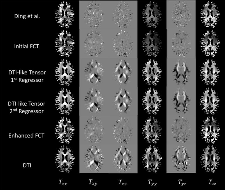
The WM-masked FCTs from one exemplar subject, computed using Ding et al.’s method and the proposed method, respectively. The actual DTs are shown for reference. Each row shows the six elements of the tensor {T_xx, T_xy, T_xz, T_yy, T_yz, T_zz}.

To better evaluate the performance of the proposed framework, especially the process of FCT enhancement, we also compute the four parameter maps {I_AD, I_RD, I_MD, I_FA} from the extracted tensors, which are computed using the three eigenvalues {λ₁, λ₂, λ₃} of the DT as follows:

$$\{\begin{array}{l}{I}_{AD}={\lambda }_1\hfill \\ I_{RD}=\left({\lambda }_2+{\lambda }_3\right)/2\hfill \\ I_{MD}=\left({\lambda }_1+{\lambda }_2+{\lambda }_3\right)/3\hfill \\ I_{FA}\sqrt{\frac{3}{2}}\sqrt{\frac{{\left({\lambda }_1-I_{MD}\right)}^2+{\left({\lambda }_2-I_{MD}\right)}^2+{\left({\lambda }_3-I_{MD}\right)}^2}{\left({\lambda }_1^2+{\lambda }_2^2+{\lambda }_3^2\right)}}\hfill \end{array}.$$ (9)

Figure 4 presents the WM-masked parameter maps using FCTs from the method of Ding et al. and different stages in the proposed framework. The parameter maps from the DTI data are also presented here as a reference. Similar to Figure 3, the proposed framework outperforms Ding et al., especially for the FA map. It can also be observed, especially for the FA map, that the DTI-like tensor has helped to refine the details in the WM regions of the enhanced FCT. This indicates that the novel strategies in the proposed framework can help improve the quality of FCTs.

Figure 4.

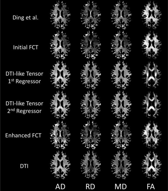
Four different WM-masked parameter maps (AD, RD, MD, FA) computed from the various tensor estimates from one exemplar subject using Ding et al.’s method and the proposed method. The DTs are shown for reference.

It is worth noting that the average computation time using the method of Ding et al. is around 10 minutes using a standard PC (CPU 3.1GHz i5, memory 24 GB 1333MHz DDR3), while it takes much more time (45 minutes) to obtain the initial FCT using our framework. This is partly due to the greater computational cost associated with the patch-based FCT computation. FCT to DT mapping using regression forest method with the auto-context model also takes about 20 minutes. Speed can be improved via parallelization.

To further quantify the similarity between predicted DTI-like tensors and the actual DTs by using Pearson’s correlation as the metric. The overall whole-brain correlation coefficient for the first and second stage mapping are 0.698±0.064 and 0.729±0.068, respectively. Using the two-tailed t-test, experiments show that there is a significant improvement between the two stages (p<0.05). The average correlation values for different ROIs based on the ICBM DTI-81 atlas are provided in Table 1. The p-values are computed using two-tailed t-tests between two stages. Significant improvement (p < 0.05) is marked with an asterisk. It can be observed that the correlation is improved in the second stage with the help of the auto-context model.

Table 1.

Pearson’s correlation values for different WM ROIs between the predicted DTI-like tensors in two stages and their actual DTs. Significant improvement (p<0.05) of the overall correlation coefficients for different ROIs between two stages is marked with asterisk.

No	ROI	First Stage	Second Stage
1*	Genu of corpus callosum	0.339±0.229	0.418±0.250
2*	Body of corpus callosum	0.290±0.187	0.338±0.233
3*	Splenium of corpus callosum	0.504±0.153	0.538±0.187
4*	Fornix	0.360±0.259	0.479±0.301
5*	R. cerebral peduncle	0.621±0.147	0.737±0.147
6*	L. cerebral peduncle	0.613±0.157	0.744±0.142
7*	R. ant. limb of int. capsule	0.650±0.159	0.758±0.157
8*	L. ant. limb of int. capsule	0.607±0.182	0.712±0.177
9*	R. post. limb of int. capsule	0.729±0.146	0.791±0.162
10*	L. post. limb of int. capsule	0.741±0.105	0.804±0.117
11*	R. retro. part of int. capsule	0.504±0.230	0.593±0.240
12*	L. retro. part of int. capsule	0.463±0.194	0.535±0.227
13*	R. ant. corona radiate	0.401±0.166	0.513±0.177
14*	L. ant. corona radiate	0.382±0.160	0.473±0.190
15*	R. sup. corona radiate	0.510±0.175	0.575±0.200
16*	L. sup. corona radiate	0.496±0.157	0.576±0.171
17*	R. post. corona radiate	0.210±0.211	0.318±0.240
18*	L. post. corona radiate	0.252±0.197	0.324±0.220
19	R. post. thalamic radiation	0.316±0.193	0.363±0.215
20	L. post. thalamic radiation	0.282±0.221	0.330±0.233
21*	R. sagittal stratum	0.218±0.181	0.283±0.229
22*	L. sagittal stratum	0.297±0.174	0.367±0.189
23*	R. external capsule	0.601±0.130	0.647±0.155
24*	L. external capsule	0.558±0.137	0.608±0.171
25*	R. cingulum (cigulate gyrus)	0.138±0.156	0.226±0.187
26*	L. cingulum (cigulate gyrus)	0.161±0.171	0.264±0.222
27*	R. cingulum (hippocampus)	0.304±0.235	0.485±0.239
28*	L. cingulum (hippocampus)	0.346±0.239	0.502±0.217
29*	R. fornix / stria terminalis	0.235±0.197	0.348±0.238
30*	L. fornix / stria terminalis	0.181±0.171	0.306±0.220
31*	R. sup. longitudinal fasciculus	0.323±0.222	0.413±0.238
32*	L. sup. longitudinal fasciculus	0.305±0.201	0.408±0.218
33*	R. sup. fronto-occipital fasciculus	0.266±0.312	0.406±0.282
34	L. sup. fronto-occipital fasciculus	0.274±0.346	0.346±0.388
35	R. inf. fronto-occipital fasciculus	0.532±0.257	0.589±0.274
36	L. inf. fronto-occipiral fasciculus	0.470±0.310	0.536±0.323
37	R. uncinate fasciculus	0.250±0.244	0.324±0.271
38	L. uncinate fasciculus	0.198±0.254	0.258±0.288
	Overall	0.393±0.199	0.480±0.219

Figure 5 presents the 3D ellipsoidal glyphs of the DTs, generated using “TVglyphview” of DTI-TK toolkit¹, with the T1-weighted image as background. It can be observed that the glyphs show reasonable similarity especially in the WM.

Figure 5.

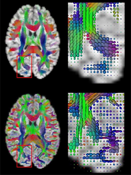
Exampler 3D ellipsoidal glyphs based on the DTI-like tensors (first row) and the actual DTs (second row).

Figure 6 shows the tractography results generated using the Diffusion toolkit and visualized using TrackVis [46]. Figure 7 and Figure 8 compare several WM fiber tracts in the left hemisphere of the brain [47]: arcuate fasciculus (AF), corpus callosum (CC), corticospinal tract (CST), inferior frontooccipital fasciculus (IFF) and inferior longitudinal fasciculus (ILF). The fiber tracts are visualized using the ParaView toolkit [48], with the brain’s inner surface presented as underlay. It can be observed that the majority of WM pathways are similar.

Figure 6.

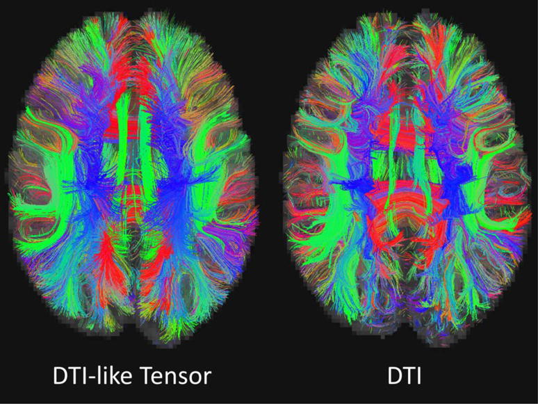
Exampler fiber tracking results based on the DTI-like tensors (left) and the actual DTs (right).

Figure 7.

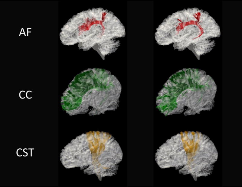
Exampler fiber tracking results based on DTI-like tensors (left) and DTI (right) for AF (arcuate fasciculus), CC (corpus callosum) and CST (corticospinal tracts).

Figure 8.

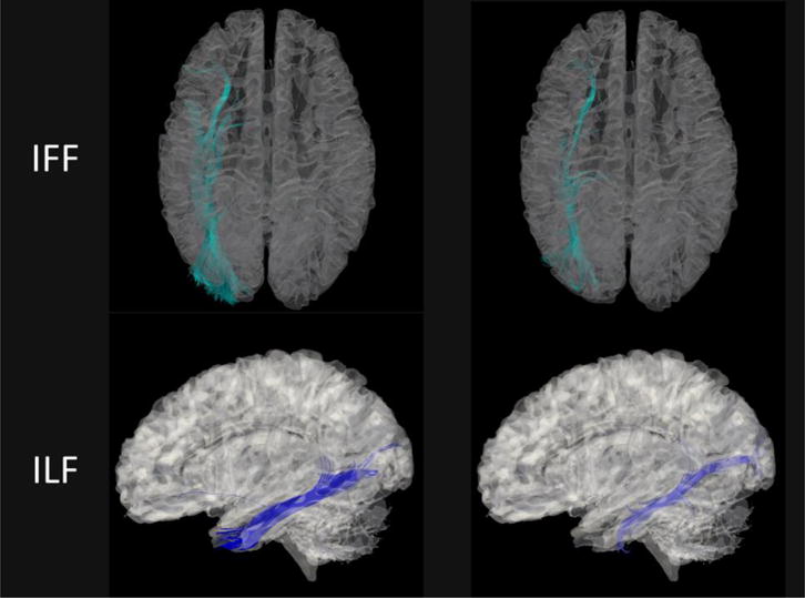
Exampler fiber tracking results based on the predicted DTI-like tensors (left) and the actual DTs (right) for IFF (inferior frontooccipital fasciculus) and ILF (inferior longitudinal fasciculus).

Furthermore, we found that the DTI-like tensors are also capable of capturing the individual variability of the brain structure from different subjects. Figure 9 presents the ILF tracts generated from DTI-like tensors of four subjects obtained using our framework. Since the subjects in HCP dataset were aligned to the MNI-152 space using only AC-PC registration [31], there are certain variations of brain structures from different subjects, especially for the ILF tracts. It can be still observed that the ILF tracts are well aligned to each subject’s WM structures, respectively.

Figure 9.

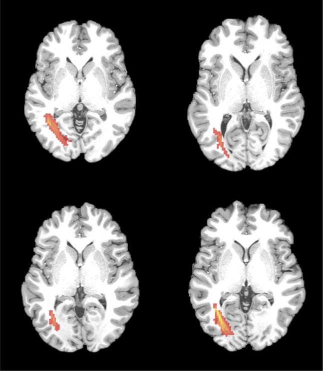
ILF (red) estimated from the predicted DTI-like tensors of four subjects.

3.2 Informative Enhanced FCT in MCI Classification

In this section, we utilize enhanced FCT for eMCI-NC identification by following the methodology introduced in Section 2.5. Note that we randomly choose the forest model trained in one fold of the cross-validation in Section 3.1 to estimate the DTI-like tensors. Experiments show that the forests of all four folds provide similar mapping capability. The estimated tensors along with the four parameter maps from the ADNI dataset can be referred from Figure 3 and Figure 4.

Leave-one-out (LOO) cross-validation was applied to verify the classification performance due to the limited sample size. For optimizing the parameters in LASSO and SVM, we used an inner LOO cross-validation on the training samples. Using FA for classification, the ACC and AUC using Ding et al.’s FCT computation method are 67.90% and 69.90%. Using the initial FCTs, the ACC and AUC are improved to 69.14% and 72.83%, which further become 70.37% and 74.85% using the enhanced FCTs. The ROC curves shown in Figure 10 indicate that the proposed framework outperforms Ding et al.’s method, and both the strategies in the initial and enhanced FCT estimations help to improve the quality. Note that in our experiments the number of NC subjects is larger than that of the eMCI subjects. To better evaluate the classification performance for unbalanced data, we also use the balanced accuracy (BAC). The BAC values for FCT using Ding et al.’s method, the initial FCTs and the enhanced FCTs are 67.31%, 68.96% and 70.33%, respectively. This is consistent with the conclusions drawn using the ACC and AUC values. It is worth noting that the experiment conducted in this section only exploits features from the WM. In the future, GM features can also be included to improve the classification performance.

Figure 10.

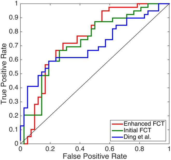
The ROC curve for the eMCI-NC classification using the initial and enhanced FCTs by the proposed framework, and the FCTs by Ding et al.’s method.

4 Discussion

4.1 Observations of fMRI in WM

There are many recent attempts in investigating WM neural activity using fMRI [19]. fMRI activations are found in corpus callosum [13], internal capsule [15, 16] and optic radiations [19]. Furthermore, Ding et al. [20, 21] showed that the spatiotemporal correlation patterns of BOLD signals in WM exhibit similar orientation information as DTI. Marussich et al. [19] reported the intrinsic hierarchical functional organization associated with WM pathways.

BOLD signals are related to vasculature, cerebral blood flow (CBF), and cerebral blood volume (CBV). Since micro blood vessels and capillary vessels are spatially distributed along the main directions of fiber bundles, the BOLD signals in WM should also have consistent spatial characteristics with DTI. This has in fact been demonstrated in Ding et al.’s work [20, 21].

4.2 DTI-Guided FCT Estimation

Following the rationale given in Section 4.1, we use the directional information given by DTs to improve FCT estimation. Considering the possibility that DTI data might not be available, we use our learning-based model for predicting DTI-like tensors.

Note that the proposed method is implemented by following an individual-subject level manner. Stated succinctly, the FCT of the input subject is obtained mostly from its corresponding rs-fMRI image information. We only utilize the group-level information when learning the forest model to predict DTI-like tensors. Still, our mapping strategy is developed to ensure the DTI-like tensors can capture the individual variability of the subjects’ brain structure, as shown in Figure 8. Furthermore, the enhanced FCTs after the guidance of DTI-like tensors can better present the local functional connectivity information in WM region.

4.3 Difference Between FCT and DT

It is worth noting that based on the current findings, the FCT and DT should be considered as two metrics with only partial similarities with each other. As they are originated from rs-fMRI and DTI respectively, and the corresponding information they represent is also different (functional and diffusion). This can also be observed in Figure 3 and Figure 4, where the obtained FCT and DT are presented. Since there is no ground-truth FCT to evaluate the current estimation, we also consider the eMCI-NC classification to compare the FCT estimated in different configurations in a quantitative evaluation manner. The classification results can prove that the novel strategies introduced in this paper are effective, and the enhanced FCTs clearly outperform the others.

4.4 Limitations and Potential Remedies

The performance of our method is limited by a number of factors.

First, the three-step framework involves aligning the initial FCT to the common space before mapping can be carried out. The predicted DTI-like tensors are warped back to the individual space for FCT enhancement. Potential registration errors may affect the accuracy of the estimated FCTs. A means to mitigate the effects of registration errors is by using a patch matching mechanism to correct for misalignment [33].

Second, FCTs are computed for the whole brain, including the GM that has much higher SNR in terms of BOLD signals than that WM. FCTs at the WM-GM boundary might be affected by the signal differences between the two tissue types. This problem can be ameliorated by using tissue segmentation information from anatomical T1 images so GM and WM can be analyzed separately.

Third, Ding et al. has presented in [20, 21] that some fiber streamlines (e.g. ILF, optic radiation and etc.) can be reconstructed from the estimated FCT. Besides, our enhanced FCTs have shown anistropy in WM regions that are more aligned to the predicted DTI-like tensors as observed in Figure 3 and Figure 4. However, unlike the DTs, it is still hard to implement fiber tracking to the whole WM regions of those obtained FCTs. We attribute this issue to the HCP data, which is multiband echo planar imaging (EPI) data with both higher spatial and temporal resolution, and thus sacrifices the SNR of BOLD signals. In future, we will test our method using more data sets with better SNR, with which we could anticipate a better FCT enhancement performance. Therefore, our ultimate goal, i.e., using FCT to conduct individualized fiber tracking, like DTI, can be achieved.

4.5 Future Works

For future clinical applications, the trained forest model can be applied to other datasets, including both healthy and patient cohorts (autism, Parkinson’s diseases, etc.). We will also test our method on task-based fMRI to investigate FCT in different states.

5 Conclusion

In this work, we have presented a novel learning-based framework that improves the quality of FCTs. We proposed a patch-based correlation measurement strategy to improve noise robustness in FCT computation. We also incorporated regression forest with the auto-context model to predict DTI-like tensors from FCTs. The FCTs are then enhanced using the information given by the predicted DTI-like tensors. Experimental results indicate that the quality of FCTs is improved. When used for AD diagnosis, the enhanced FCTs also improves the classification accuracy.

References

- 1.Fox MD, Greicius M. Clinical applications of resting state functional connectivity. Frontiers in systems neuroscience. 2010;4:19. doi: 10.3389/fnsys.2010.00019. [DOI] [PMC free article] [PubMed] [Google Scholar]
- 2.Gore JC. Principles and practice of functional MRI of the human brain. The Journal of Clinical Investigation. 2003;112(1):4–9. doi: 10.1172/JCI19010. [DOI] [PMC free article] [PubMed] [Google Scholar]
- 3.Greve DN, et al. A survey of the sources of noise in fMRI. Psychometrika. 2013;78(3):396–416. doi: 10.1007/s11336-012-9294-0. [DOI] [PubMed] [Google Scholar]
- 4.Filippi M. fMRI techniques and protocols. Springer; 2009. [Google Scholar]
- 5.Biswal B, et al. Functional connectivity in the motor cortex of resting human brain using echo-planar mri. Magnetic Resonance in Medicine. 1995;34(4):537–541. doi: 10.1002/mrm.1910340409. [DOI] [PubMed] [Google Scholar]
- 6.Nonaka H, et al. Microvasculature of the human cerebral white matter: arteries of the deep white matter. Neuropathology. 2003;23(2):111–118. doi: 10.1046/j.1440-1789.2003.00486.x. [DOI] [PubMed] [Google Scholar]
- 7.Raichle ME, et al. A default mode of brain function. Proceedings of the National Academy of Sciences. 2001;98(2):676–682. doi: 10.1073/pnas.98.2.676. [DOI] [PMC free article] [PubMed] [Google Scholar]
- 8.Basser PJ, Mattiello J, LeBihan D. MR diffusion tensor spectroscopy and imaging. Biophysical Journal. 1994;66(1):259. doi: 10.1016/S0006-3495(94)80775-1. [DOI] [PMC free article] [PubMed] [Google Scholar]
- 9.Alexander AL, et al. Diffusion tensor imaging of the brain. Neurotherapeutics. 2007;4(3):316–329. doi: 10.1016/j.nurt.2007.05.011. [DOI] [PMC free article] [PubMed] [Google Scholar]
- 10.Basser PJ, et al. In vivo fiber tractography using DT-MRI data. Magnetic Resonance in Medicine. 2000;44(4):625–632. doi: 10.1002/1522-2594(200010)44:4<625::aid-mrm17>3.0.co;2-o. [DOI] [PubMed] [Google Scholar]
- 11.Bullmore E, Sporns O. Complex brain networks: graph theoretical analysis of structural and functional systems. Nature Reviews Neuroscience. 2009;10(3):186–198. doi: 10.1038/nrn2575. [DOI] [PubMed] [Google Scholar]
- 12.Tettamanti M, et al. Interhemispheric transmission of visuomotor information in humans: fMRI evidence. Journal of Neurophysiology. 2002;88(2):1051–1058. doi: 10.1152/jn.2002.88.2.1051. [DOI] [PubMed] [Google Scholar]
- 13.D’Arcy RC, et al. Exploratory data analysis reveals visuovisual interhemispheric transfer in functional magnetic resonance imaging. Magnetic Resonance in Medicine. 2006;55(4):952–958. doi: 10.1002/mrm.20839. [DOI] [PubMed] [Google Scholar]
- 14.Mazerolle EL, D’Arcy RC, Beyea SD. Detecting functional magnetic resonance imaging activation in white matter: interhemispheric transfer across the corpus callosum. BMC Neuroscience. 2008;9(1):1. doi: 10.1186/1471-2202-9-84. [DOI] [PMC free article] [PubMed] [Google Scholar]
- 15.Mosier KM, et al. Lateralization of cortical function in swallowing: a functional MR imaging study. American Journal of Neuroradiology. 1999;20(8):1520–1526. [PMC free article] [PubMed] [Google Scholar]
- 16.Gawryluk JR, et al. Investigation of fMRI activation in the internal capsule. BMC Neuroscience. 2011;12(1):1. doi: 10.1186/1471-2202-12-56. [DOI] [PMC free article] [PubMed] [Google Scholar]
- 17.Mazerolle EL, et al. Sensitivity to white matter FMRI activation increases with field strength. PloS One. 2013;8(3):e58130. doi: 10.1371/journal.pone.0058130. [DOI] [PMC free article] [PubMed] [Google Scholar]
- 18.Gawryluk JR, Mazerolle EL, D’Arcy RC. Does functional MRI detect activation in white matter? A review of emerging evidence, issues, and future directions. Frontiers in Neuroscience. 2014;8:239. doi: 10.3389/fnins.2014.00239. [DOI] [PMC free article] [PubMed] [Google Scholar]
- 19.Marussich L, et al. Mapping white-matter functional organization at rest and during naturalistic visual perception. NeuroImage. 2016 doi: 10.1016/j.neuroimage.2016.10.005. [DOI] [PMC free article] [PubMed] [Google Scholar]
- 20.Ding Z, et al. Spatio-temporal correlation tensors reveal functional structure in human brain. PloS One. 2013;8(12):e82107. doi: 10.1371/journal.pone.0082107. [DOI] [PMC free article] [PubMed] [Google Scholar]
- 21.Ding Z, et al. Visualizing functional pathways in the human brain using correlation tensors and magnetic resonance imaging. Magnetic Resonance Imaging. 2016;34(1):8–17. doi: 10.1016/j.mri.2015.10.003. [DOI] [PMC free article] [PubMed] [Google Scholar]
- 22.Huettel SA, Song AW, McCarthy G. Functional magnetic resonance imaging. Vol. 1. Sinauer Associates Sunderland; 2004. [Google Scholar]
- 23.Wise RG, et al. Resting fluctuations in arterial carbon dioxide induce significant low frequency variations in BOLD signal. Neuroimage. 2004;21(4):1652–1664. doi: 10.1016/j.neuroimage.2003.11.025. [DOI] [PubMed] [Google Scholar]
- 24.Zikic D, Glocker B, Criminisi A. Atlas encoding by randomized forests for efficient label propagation. MICCAI; 2013. pp. 66–73. [DOI] [PubMed] [Google Scholar]
- 25.Zhang L, et al. Automatic labeling of MR brain images by hierarchical learning of atlas forests. Medical Physics. 2016;43(3):1175–1186. doi: 10.1118/1.4941011. [DOI] [PMC free article] [PubMed] [Google Scholar]
- 26.Zhang L, et al. Concatenated Spatially-localized Random Forests for Hippocampus Labeling in Adult and Infant MR Brain Images. Neurocomputing. 2016 doi: 10.1016/j.neucom.2016.05.082. [DOI] [PMC free article] [PubMed] [Google Scholar]
- 27.Huynh T, et al. Estimating CT Image From MRI Data Using Structured Random Forest and Auto-Context Model. IEEE Transactions on Medical Imaging. 2016;35(1):174–183. doi: 10.1109/TMI.2015.2461533. [DOI] [PMC free article] [PubMed] [Google Scholar]
- 28.Tu Z, Bai X. Auto-context and its application to high-level vision tasks and 3D brain image segmentation. IEEE transactions on pattern analysis and machine intelligence. 2010;32(10):1744–57. doi: 10.1109/TPAMI.2009.186. [DOI] [PubMed] [Google Scholar]
- 29.Van Essen DC, et al. The WU-Minn human connectome project: an overview. Neuroimage. 2013;80:62–79. doi: 10.1016/j.neuroimage.2013.05.041. [DOI] [PMC free article] [PubMed] [Google Scholar]
- 30.Mueller SG, et al. The Alzheimer’s disease neuroimaging initiative. Neuroimaging Clinics of North America. 2005;15(4):869–877. doi: 10.1016/j.nic.2005.09.008. [DOI] [PMC free article] [PubMed] [Google Scholar]
- 31.Glasser MF, et al. The minimal preprocessing pipelines for the Human Connectome Project. Neuroimage. 2013;80:105–124. doi: 10.1016/j.neuroimage.2013.04.127. [DOI] [PMC free article] [PubMed] [Google Scholar]
- 32.Jenkinson M, et al. FSL. Neuroimage. 2012;62(2):782–790. doi: 10.1016/j.neuroimage.2011.09.015. [DOI] [PubMed] [Google Scholar]
- 33.Heinrich MP, et al. MIND: Modality independent neighbourhood descriptor for multi-modal deformable registration. Medical Image Analysis. 2012;16(7):1423–1435. doi: 10.1016/j.media.2012.05.008. [DOI] [PubMed] [Google Scholar]
- 34.Wang L, et al. LINKS: Learning-based multi-source IntegratioN frameworK for Segmentation of infant brain images. Neuroimage. 2015;108:160–172. doi: 10.1016/j.neuroimage.2014.12.042. [DOI] [PMC free article] [PubMed] [Google Scholar]
- 35.Zhang J, et al. Brain atlas fusion from high-thickness diagnostic magnetic resonance images by learning-based super-resolution. Pattern Recognition. 2017;63:531–541. doi: 10.1016/j.patcog.2016.09.019. [DOI] [PMC free article] [PubMed] [Google Scholar]
- 36.Breiman L. Machine Learning. Springer; 2001. Random forests. [Google Scholar]
- 37.Kontschieder P, et al. International Conference on Computer Vision. IEEE; 2011. Structured class-labels in random forests for semantic image labelling. [Google Scholar]
- 38.Aganj I, et al. Reconstruction of the orientation distribution function in single- and multiple-shell q-ball imaging within constant solid angle. Magnetic Resonance in Medicine. 2010;64(2):554–566. doi: 10.1002/mrm.22365. [DOI] [PMC free article] [PubMed] [Google Scholar]
- 39.Tuch DS. Q-ball imaging. Magnetic resonance in medicine. 2004;52(6):1358–1372. doi: 10.1002/mrm.20279. [DOI] [PubMed] [Google Scholar]
- 40.Frackowiak RS, et al. Human brain function. Academic press; 2004. [Google Scholar]
- 41.Hagmann P, et al. Mapping the structural core of human cerebral cortex. PLoS Biol. 2008;6(7):e159. doi: 10.1371/journal.pbio.0060159. [DOI] [PMC free article] [PubMed] [Google Scholar]
- 42.Chen X, et al. High-order resting-state functional connectivity network for MCI classification. Human brain mapping. 2016 doi: 10.1002/hbm.23240. [DOI] [PMC free article] [PubMed] [Google Scholar]
- 43.Chen X, et al. Extraction of Dynamic Functional Connectivity from Brain Grey Matter and White Matter for MCI Classification. Human Brain Mapping. 2017 doi: 10.1002/hbm.23711. [DOI] [PMC free article] [PubMed] [Google Scholar]
- 44.Saeys Y, Inza I, Larrañaga P. A review of feature selection techniques in bioinformatics. Bioinformatics. 2007;23(19):2507–2517. doi: 10.1093/bioinformatics/btm344. [DOI] [PubMed] [Google Scholar]
- 45.Cortes C, Vapnik V. Support-vector networks. Machine Learning. 1995;20(3):273–297. [Google Scholar]
- 46.Wang R, et al. Diffusion toolkit: a software package for diffusion imaging data processing and tractography. Proc Intl Soc Mag Reson Med. 2007 [Google Scholar]
- 47.Catani M, de Schotten MT. A diffusion tensor imaging tractography atlas for virtual in vivo dissections. Cortex. 2008;44(8):1105–1132. doi: 10.1016/j.cortex.2008.05.004. [DOI] [PubMed] [Google Scholar]
- 48.Ahrens J, et al. 36-ParaView: An End-User Tool for Large-Data Visualization. The Visualization Handbook; 2005. p. 717. [Google Scholar]