Exposure to seismic air gun signals causes physiological harm and alters behavior in the scallop Pecten fumatus

Significance

Seismic surveys are used around the world as the primary means to explore for oil and gas deposits. Almost nothing is known regarding the impact of these sound signals on marine invertebrates. In this study, the physiological and behavioral effects of exposure on a commercially important bivalve, the scallop, were quantified. Following a field-based air gun exposure regime, exposed scallops were found to have significantly increased mortality rates; disrupted behavioral patterns and reflex responses, both during and following exposure; and altered hemolymph biochemistry, physiology, and osmoregulation capacity. These results indicate that air gun exposure has a harmful impact on scallops and raises concern over the impact on bivalves, due to their global ecological and economic importance.

Abstract

Seismic surveys map the seabed using intense, low-frequency sound signals that penetrate kilometers into the Earth’s crust. Little is known regarding how invertebrates, including economically and ecologically important bivalves, are affected by exposure to seismic signals. In a series of field-based experiments, we investigate the impact of exposure to seismic surveys on scallops, using measurements of physiological and behavioral parameters to determine whether exposure may cause mass mortality or result in other sublethal effects. Exposure to seismic signals was found to significantly increase mortality, particularly over a chronic (months postexposure) time scale, though not beyond naturally occurring rates of mortality. Exposure did not elicit energetically expensive behaviors, but scallops showed significant changes in behavioral patterns during exposure, through a reduction in classic behaviors and demonstration of a nonclassic “flinch” response to air gun signals. Furthermore, scallops showed persistent alterations in recessing reflex behavior following exposure, with the rate of recessing increasing with repeated exposure. Hemolymph (blood analog) physiology showed a compromised capacity for homeostasis and potential immunodeficiency, as a range of hemolymph biochemistry parameters were altered and the density of circulating hemocytes (blood cell analog) was significantly reduced, with effects observed over acute (hours to days) and chronic (months) scales. The size of the air gun had no effect, but repeated exposure intensified responses. We postulate that the observed impacts resulted from high seabed ground accelerations driven by the air gun signal. Given the scope of physiological disruption, we conclude that seismic exposure can harm scallops.

Seismic surveys are used to explore the geological structure of the seafloor, using an array of air guns that are slowly (ca. 3 km⋅h⁻¹ to 4 km⋅h⁻¹) towed up and down parallel track lines, generating intense, low-frequency acoustic signals every 8 s to 15 s (every 20 m to 30 m) through the instantaneous release of highly compressed air (1). Surveys operate continuously 24 h a day and last from weeks to months, covering an area hundreds to thousands of square kilometers, with a nearly ubiquitous global distribution. Seismic surveys are commonly used to explore for subseafloor oil and gas deposits, but are also necessary for identifying sites for carbon sequestration, a developing means to cope with anthropogenic production of CO₂ (2).

Seismic signals have a potentially important, yet poorly understood, anthropogenic impact on life in the marine environment. To date, the effects of exposure on whales have received considerable attention (3), and fishes have received somewhat less attention (4). Even less is understood regarding the effect of exposure on invertebrates (5). Field-based experiments have rarely been conducted on invertebrates, and the limited available evidence shows little effect on crab and lobster larvae, while zooplankton show a high level of taxa-specific mortality (6–8). Tank-based experiments simulating exposure have resulted in high levels of damage in several molluscs, including scallop veliger larvae (9) and several species of squid and octopus (10–12), although it is unclear how laboratory experiments conducted in tanks may translate into the field (13, 14).

Among marine invertebrates, bivalves would seem to be particularly vulnerable, as their benthic and largely sessile habit leaves little capacity to avoid the waterborne and groundborne energy of seismic signals. Even the relatively mobile scallop, which swims using jet propulsion, has little chance of escaping exposure, as their energetically demanding form of locomotion leaves even the most competent swimming species depleted after about 4 min of swimming, during which they can cover, at most, a modest 30 m (15, 16).

Bivalves perform a diversity of roles within an ecosystem, including improving water quality through reduction of turbidity, thus increasing light availability for underwater plants; exerting both top-down and bottom-up control on phytoplankton, ameliorating the anthropogenic nutrient inputs that drive eutrophication in coastal waters; and the bio-deposition of pelagic primary production nutrients into benthic systems (17). Bivalves also have substantial socioeconomic value, making potential harm a considerable issue. Global production of bivalves has been constantly increasing over the past 6 decades, as the total annual production (capture + aquaculture) of mussel, oyster, scallop, and clam fisheries has increased from 1 million tons in 1950 to over 14 million tons in 2014, with an annual value of nearly US$17 billion (18). Not only are bivalves increasingly relied upon for food security, but a diverse range of value-added industries, including pharmaceuticals, agriculture, building materials, cosmetics, clothing, and jewelry, have developed to take advantage of fishery by-products (19). This increase in global demand has driven advancements of the bivalve mariculture industry, recognized as one the most environmentally sound and sustainable forms of aquaculture, since bivalve aquaculture does not require the addition of food nutrients into a system which may drive eutrophication, as in other forms of aquaculture (19, 20). Rather, bivalves actually improve water quality through biofiltration and biodeposition of organic matter from the water column, assisting in the feeding of other benthic organisms (20). Bivalves have also been incorporated into finfish aquaculture in an effort to reduce the nutrient load, a practice called integrated multitrophic aquaculture (21).

There is considerable overlap between areas supporting bivalve aquaculture and capture fisheries and areas of interest for seismic exploration (Fig. 1). This overlap can result in conflict, as was the case when a scallop mass mortality in Australia’s Bass Strait, in which the fishing industry estimated a loss of 24,000 tons of scallops, was anecdotally attributed to a seismic survey. Conflicts between users of marine resources are not new, with oil and fishery industries frequently at odds worldwide and a variety of regulatory and resolution approaches adopted to mitigate the tension (22). Despite the rise in prominence of various forms of renewable energy, oil and gas consumption continues to grow. Exploration using marine seismic surveys will be necessary to meet demand and to ameliorate the resulting carbon emissions, requiring the expansion of surveys into areas of high biodiversity (23) and high-latitude polar seas, particularly the Arctic (24, 25), where bivalves live long, slow lives (i.e., slow to reach reproductive age) with narrow physiological constraints (26).

Fig. 1.

Estimated global undiscovered oil [million barrels of oil equivalent (MMBOE) scale] and bivalve (mussels, oysters, scallops, clams) production (tonnes scale). Undiscovered oil estimates were sourced from US Geological Survey (71). Bivalve capture and aquaculture fishery production data were sourced from Food and Agriculture Organization (18).

Here, we use a field-based approach to assess the impact of exposure of a single air gun on the scallop Pecten fumatus. Scallops were exposed to air gun signals in a field setting designed to emulate a survey in real-world conditions, and were assessed for mortality, physiology, and behavioral responses over acute (i.e., hours to days postexposure) and chronic (i.e., months postexposure) scales to provide detailed and systematic time series sampling. To evaluate whether exposure causes mortality, mortality rates were assessed through observation at time points ranging from immediately after exposure to 4 mo postexposure. Video recordings of scallops were used to analyze behavior before, during, and following exposure to determine whether air gun signals result in the behavioral alterations posited by the mortality hypothesis. Following exposure, the scallops’ recessing reflexes were evaluated by measuring the time taken to recess into the substrate, a state considered the “natural” position of P. fumatus (27) and other scallops with a convex lower valve and a flattened upper valve (28, 29). Sublethal physiological effects were quantified through assays of the cellular and humoral components of the hemolymph, the invertebrate analog to vertebrate blood, with measurement of the pH, number of circulating hemocytes, and hemolymph biochemistry compared between treatments. Although there are few investigations into the various parameters of pectinid hemolymph, scallops are osmoconformers and would not be expected to show considerable variation in hemolymph chemistry (i.e., pH, ion concentration) when maintained in stable seawater conditions. The general bivalve hemocyte response, based on a review of studies of mussels, oysters, and clams, is much more dynamic, responding to a range of biotic (reproductive state, nutritional condition, size/age) and abiotic (water temperature, salinity, exposure to pathogens) factors (30). The typical bivalve response to acute environmental stressors described in ref. 30 is an increase in hemocyte numbers, either through cell proliferation or mobilization of cells from tissues to circulation, although some stressors elicit a decrease in hemocyte numbers, driven by cell death or immobilization within tissues. Scallops show a similar response following exposure to environmental pollution (31, 32). We hypothesize that P. fumatus will show a response to seismic air gun exposure similar to the response observed in scallops and other bivalves in response to other acute stressors: a stable pH and biochemistry and a transient increase in circulating hemocytes following exposure, with a return to baseline or control levels shortly (i.e., with days) after exposure.

Combining an assessment of mortality rates, analysis of behavioral responses in the field during real-world exposure, and quantification of physiological responses to exposure to seismic air gun signals will provide a conclusive understanding of how scallops are affected and advance our understanding of the potential impact exploration of the seabed may have for bivalve populations.

Results

Seismic Exposure.

The calculated sound exposure levels (SEL) and measured ground roll acceleration for the different scallop experimental regimes are given in Table 1, with the best fit curves used to determine values shown in Fig. S1. Compared with the modeled levels of a hypothetical 3,065-in³ full-scale array (Table 2 and Fig. S2), the scallops exposed to one pass in the present study experienced exposures equivalent to a large commercial array passing within a 114- to 875-m range, the scallops exposed to two passes experienced the equivalent of a full scale array at 114- to 500-m range, and the scallops exposed to four passes received the equivalent of a full scale array passing at 114- to 275-m range. These range bounds were derived from the spread of comparative ranges when comparing our experimental air gun to the hypothetical air gun array, for single-shot SEL, cumulative SEL, and maximum values of the maximum magnitude of the single-shot ground acceleration vector. Lower range bounds were set by ground acceleration, and upper range bounds were set by cumulative SEL.

Table 1.

Calculated exposure values for the scallop experiments

Experiment	Max PP	Shots within 3dB max PP	Shots > 190 PP	Max SEL	Shots within 3 dB max SEL	Shots > 180 SEL	Max SELcum	Median SELcum	No. of shots	Min GR	Max GR
E-1 45-in3 pass 1	191	40	14	181	3	1	189	189	167	0.29	37.22
E-1 45-in3 passes 1 and 2	191	63	23	181	5	1	191	191	226	0.29	37.27
E-1 45-in3 passes 1 to 4	191	148	52	181	8	2	194	194	393	0.29	37.57
E-2 150-in3 pass 1	212	2	40	187	2	5	193	192	128	0.27	31.60
E-2 150-in3 passes 1 and 2	213	2	71	188	2	8	195	194	195	0.27	35.37
E-2 150-in3 passes 1 to 4	213	3	151	188	4	19	198	198	309	0.27	36.39
E-3 150-in3 pass 1	213	1	26	188	1	3	191	188	54	0.68	35.54
E-3 150-in3 passes 1 and 2	213	2	61	188	2	6	195	193	115	0.68	36.60
E-3 150-in3 passes 1 to 4	213	2	140	188	2	6	197	196	251	0.67	36.60

Given are maximum (Max) peak to peak [PP, in decibels relative to (dB re) 1 µPa]; number of signals within 3 dB of maximum PP at any cage; number of signals at any cage > 190 dB re 1 µPa PP; maximum SEL (dB re 1 μPa²·s); maximum shots/cage within 3 dB of maximum SEL; maximum shots/cage with signals > 180 dB re 1 µPa²·s SEL; maximum cumulative SEL (SEL_cum, dB re 1 μPa²·s); median SEL_cum across cages; number of shots/treatment; estimated minimum (Min GR) magnitude ground roll (GR)/treatment as measured on the seabed via geophone (meters per second squared); and estimated maximum (Max GR) magnitude ground roll/treatment as measured on the seabed via geophone (meters per second squared).

Fig. S1.

Measured parameters of air gun signals from seismic exposure experiments. (A) Measured sound exposure from trial 3 (2.46-L air gun) with the fitted curves shown (red, fixed source level; blue, floating source level). (B) Magnitude of maximum total ground roll expressed in decibel format with the single fitted curve, using data from all three experiments. The different colors represent different receiver locations; the symbols represent the air gun run.

Table 2.

Comparison of experimental scallop exposures and estimated equivalent range of hypothetical seismic survey, giving experimental regime, estimated exposure received during that experiment, and the estimated range this exposure occurred from a commercial array

Experiment	Max SEL	RangeE, m	Median SELcum	RangeE, m	Max GR (linear)	RangeE, m
2013 pass 1	181	250	189	725	37.2	114
2013 pass 2	181	250	191	500	37.3	114
2013 pass 4	181	250	194	275	37.6	118
2013 passes 1+2			196	200
2013 passes 1+2+4			197	175
2014 pass 1	187	150	192	400	31.6	129
2014 pass 2	188	150	194	275	35.4	117
2014 pass 4	188	150	198	200	36.4	120
2014 passes 1+2			196	175
2014 passes 1+2+4			200	100
2015 pass 1	188	150	188	875	35.5	117
2015 pass 2	188	150	193	325	36.6	115
2015 pass 4	188	150	196	175	36.6	115
2015 passes 1+2			194	275
2015 passes 1+2+4			198	125

The experiments are labeled by year (2013, 2014, and 2015) with one, two, and four passes within an experiment, with cumulative SEL from multiple passes indicated by pass 1+2 and pass 1+2+4. The estimated exposures are of maximum SEL experience; median cumulative SEL; and maximum magnitude of ground roll acceleration. Units are as follows: SEL and SEL_cum, dB re 1 µPa²·s; ground roll (GR), meters per second squared.

Fig. S2.

(A) Estimated ground roll for a large commercial seismic source with nearest sail line. (B) For the nearest sail line, maximum SEL (black curve) for any sail line and cumulative SEL (red curve) for the five sail lines used in modeling.

Mortality.

The cumulative mortality at the conclusion of the 2013 experiment (i.e., day 120 postexposure) was 3.8% for control zero-pass scallops, 9.4% for one-pass scallops, 11.3% for two-pass scallops, and 14.8% for four-pass scallops. In the 2014 experiment, cumulative mortality rates at day 120 were similar (P = 0.48), with 3.6% in the control zero-pass treatment, 11.3% in one-pass treatment, 16.1% in two-pass treatment, and 17.5% in four-pass treatment.

The number of passes scallops were subjected to significantly increased the cumulative number of mortalities (P = 0.009). Exposure also significantly increased the probability of mortality over time (P < 0.001), with daily odds of mortality 0.1%, 1.2%, and 1.3% higher in scallops exposed to one, two, and four passes, respectively, relative to that of controls.

In the 2015 experiment, mortality rates were 5% in control scallops and 20% in exposed scallops at day 14. At day 120, both treatments, the control zero-pass scallops and the four-pass scallops, were found to have suffered 100% mortality. This loss was not attributed to seismic exposure, as the control group also suffered complete mortality.

Behavior and Reflexes.

Qualitative analysis of video showed no evidence to support the hypothesis that seismic exposure promoted energetically expensive behaviors. In the 2014 experiment, out of 51 observed individual scallops, only four instances of swimming were observed between two individuals, which were brief (<5 s) and appeared either as responses to movements of other scallops or to adjust positioning. In the 2015 experiment, none of the 19 scallops were observed to swim. There was also no evidence of extended valve closure, as only two individuals, one each in 2014 and 2015, were observed to remain closed throughout observation. This observation was further tested by comparing tentacle state (extended, partially retracted, retracted) during preexposure, intraexposure, and postexposure time periods (Table S1), with no significant relationship between exposure and tentacle state found.

Table S1.

Effect of seismic exposure on tentacle behavior in scallops, reported as percentage of observation time with tentacles extended, partially retracted or retracted during preexposure, intraexposure, and postexposure periods during the winter 2014 150-in³ experiment and the summer 2015 150-in³ experiment

	Preexposure			Intraexposure			Postexposure
Treatment	Extended, %	Partially retracted, %	Retracted, %	Extended, %	Partially retracted, %	Retracted, %	Extended, %	Partially retracted, %	Retracted, %
2014
0-pass	94.35 ± 1.73 (n = 14)	3.87 ± 1.35 (n = 14)	1.78 ± 0.74 (n = 14)	92.57 ± 2.10 (n = 15)	5.84 ± 2.18 (n = 15)	1.59 ± 0.49 (n = 15)	89.90 ± 6.02 (n = 15)	9.40 ± 5.58 (n = 15)	0.70 ± 0.47 (n = 15)
1-pass	88.69 ± 8.16 (n = 12)	1.93 ± 0.65 (n = 12)	9.38 ± 8.27 (n = 12)	88.96 ± 8.15 (n = 12)	2.40 ± 0.93 (n = 12)	8.64 ± 8.30 (n = 12)	89.39 ± 8.97 (n = 11)	1.52 ± 0.76 (n = 11)	9.09 ± 9.09 (n = 11)
2-pass	91.77 ± 2.86 (n = 8)	3.01 ± 1.97 (n = 8)	5.22 ± 2.79 (n = 8)	97.95 ± 1.15 (n = 8)	1.89 ± 1.12 (n = 8)	0.16 ± 0.16 (n = 8)	99.10 ± 0.40 (n = 8)	0.90 ± 0.40 (n = 8)	0.0 ± 0.0 (n = 8)
4-pass	88.72 ± 1.88 (n = 8)	7.86 ± 1.48 (n = 8)	3.42 ± 0.89 (n = 8)	93.56 ± 3.26 (n = 8)	3.02 ± 1.04 (n = 8)	3.42 ± 2.44 (n = 8)	87.69 ± 7.57 (n = 8)	11.38 ± 7.68 (n = 8)	0.93 ± 0.69 (n = 8)
2015
0-pass	89.9 ± 3.41 (n = 12)	6.85 ± 2.06 (n = 12)	3.25 ± 1.52 (n = 12)	93.45 ± 3.10 (n = 12)	5.88 ± 3.03 (n = 12)	0.66 ± 0.35 (n = 12)	88.42 ± 0.05 (n = 11)	9.68 ± 0.04 (n = 11)	1.90 ± 0.02 (n = 11)
4-pass	70.07 ± 17.81 (n = 7)	14.49 ± 12.78 (n = 7)	15.44 ± 14.12 (n = 7)	66.75 ± 17.20 (n = 7)	17.53 ± 12.46 (n = 7)	15.72 ± 14.08 (n = 7)	66.36 ± 20.99 (n = 6)	7.32 ± 6.96 (n = 6)	26.32 ± 17.51 (n = 6)

Quantitative analysis of behavior during exposure showed a significant reduction (P < 0.001; Table S2) in the occurrence of classic behaviors. This reduction was specifically in response to exposure, as no differences were observed in the periods before (P = 0.38) or following (P = 0.14) exposure.

Table S2.

Effect of seismic exposure on the occurrence of classic and nonclassic behavior in scallops, during preexposure, intraexposure, and postexposure periods during seismic air gun runs during the winter 2014 150-in³ experiment and the summer 2015 150-in³ experiment

	Pre-exposure			Intraexposure			Postexposure
Treatment	Classic	Nonclassic	Time	Classic	Nonclassic	Time	Classic	Nonclassic	Time
2014
0-pass	40 (n = 19)	0 (n = 19)	4 h 48 min 6 s	36 (n = 18)	0 (n = 18)	5 h 11 min 36 s	27 (n = 19)	0 (n = 19)	4 h 5 min 10 s
1-pass	23 (n = 16)	0 (n = 16)	3 h 18 min 12 s	21 (n = 16)	29 (n = 16)	7 h 36 min 48 s	13 (n = 14)	2 (n = 14)	3 h 31 min 38 s
2-pass	3 (n = 8)	0 (n = 8)	2 h 23 min 11 s	0 (n = 8)	35 (n = 8)	1 h 54 min 29 s	6 (n = 8)	0 (n = 8)	2 h 7 min 3 s
4-pass	21 (n = 8)	0 (n = 8)	3 h 44 min 16 s	4 (n = 8)	22 (n = 8)	1 h 36 min 6 s	11 (n = 8)	0 (n = 8)	2 h 3 min 46 s
2015
0-pass	24 (n = 12)	0 (n = 12)	1 h 42 min 36 s	22 (n = 12)	0 (n = 12)	3 h 16 min 0 s	16 (n = 12)	0 (n = 12)	1 h 44 min 28 s
4-pass	3 (n = 7)	0 (n = 7)	49 min 51 s	10 (n = 7)	21 (n = 7)	1 h 35 min 59 s	2 (n = 7)	1 (n = 7)	2 h 12 min 5 s

In addition, a novel, nonclassic behavior, best described as a velar flinch, was observed (see Movie S1). This behavior was characterized by a rapid retraction of the velum and was distinct from the classic “cough” or “close” in that the upper valve, tentacles, and mantle were maintained in their “normal” resting state, unchanged relative to their position before the air gun signal. Rather, the velum was rapidly sucked in and then returned to position, with the whole behavior lasting less than 1 s. The behavior was observed exclusively in response to air gun signals at a maximum range of ∼350 m and continued to occur as the vessel approached. It was commonly observed just before the audible air gun signal, likely in response to the ground roll detected by the geophones. Velar flinches were the only observed behavior categorized as nonclassic and were significantly more frequent (P = 0.002) in two-pass scallops and four-pass scallops, in which they were observed in 100% and 75% of individuals, respectively, than in one-pass scallops, in which they were observed in 50% of individuals.

Recessing time showed a significant response to exposure in all three experiments, with increasing levels of exposure resulting in increasingly rapid recessing. For the 2013 experiment [χ²(3) = 18.06, n = 131, P < 0.001], four-pass scallops were found to recess significantly faster than both zero-pass and one-pass treatments (Fig. 2A). For the 2014 experiment, the recessing test was performed twice: immediately after exposure, as in the 2013 experiment, and again just before the day 120 sampling point. For the first test (Fig. 2B), there was a significant difference in time to recessing [χ²(3) = 16.33, n = 146, P < 0.001], with four-pass and two-pass scallops recessing significantly faster than zero-pass scallops. In the second recessing test for the 2014 experiment (Fig. 2C), conducted before day 120, four-pass scallops recessed significantly faster than zero-pass scallops [χ²(3) = 8.66, n = 55, P = 0.034]. For the 2015 experiment (Fig. 2D), the recessing test was only performed immediately after air gun exposure, due to mortality of all scallops before the 120-d sample point, and, again, the recessing rate was significantly different [χ²(1) = 13.30, n = 65, P < 0.001], with four-pass scallops recessing more quickly.

Fig. 2.

Effect of seismic exposure on the recessing reflex of scallops, in the (A) winter 2013 45-in³ experiment, (B) winter 2014 150-in³ experiment, (C) winter 2014 150-in³ experiment at day 120, and (D) summer 2015 150-in³ experiment. Within each experiment, significantly different curves as determined using logrank (Mantel−Cox) tests are indicated by differing letters.

Hemolymph Physiology and Biochemistry.

In the winter 2013 experiment (Fig. 3A) on dredge-collected scallops, both exposure and sample time had a significant effect on hemocyte counts [F(6,182) = 3.54, P = 0.002], with control scallops showing significantly higher counts than exposed scallops immediately following exposure, with the number of hemocytes of zero-pass control scallops 73% and 75% greater than that of two- and four-pass scallops, respectively. At day 14, a slight decline in mean hemocyte numbers in zero-pass control scallops resulted in no significant differences found between control and exposed treatments. At day 120, the mean total hemocyte count of zero-pass control, one-pass, and two-pass scallops increased significantly from the levels recorded at days 0 and 14, whereas four-pass scallops remained at a similar level. The degree of increase differed, however, as zero-pass control scallops had 60 to 90% more hemocytes at day 120 than the three exposed treatments.

Fig. 3.

Effect of seismic exposure on scallop hemolymph biochemistry, with (A) mean ± SEM total hemocyte counts and (B) mean ± SEM hemolymph pH by exposure level in the winter 2013 45-in³ air gun experiment, the winter 2014 150-in³ air gun experiment, and the summer 2015 150-in³ air gun experiment. For each experiment, significant differences in response to an interaction between exposure time and sample time are indicated with differing lowercase letters, and significant differences between exposure level are indicated with a horizontal bar.

In the winter 2014 experiment using hand-collected scallops, the interaction between exposure level and sample time was again significant [F(6,174) = 17.69, P < 0.001], although, in this experiment, no difference was found in the number of hemocytes between zero-pass controls and any of the exposure treatments at day 0. At day 14, four-pass scallops had a 41% higher total hemocyte count than zero-pass controls, a difference that was significant. A similar response was observed in the 2015 experiment, which was conducted in the summer using hand-collected scallops, with four-pass scallops showing 21% higher total hemocyte count [t(33.3) = 2.44, P = 0.03] at day 14. At day 120 in the 2014 experiment, zero-pass control scallops maintained a similar hemocyte count to the previous sample points, whereas one-pass, two-pass, and four-pass scallops showed a significant decline to levels 40 to 50% of that of the control treatment.

Comparison of hemolymph pH (Fig. 3B) values for the winter 2013 experiment using scallops collected via dredge showed a significant interaction with air gun passes and sample time [F(6,189) = 2.307, P = 0.036], with pairwise comparison indicating that, at day 0, one-pass scallops had a significantly higher pH than the zero-, two-, and four-pass scallops, which was the only difference between treatments at the three sample points in the experiment. The general trend observed across the three sample points was alkaline pH values at day 0 (>8.00 for all scallops), to moderately alkaline values at day 14 (between 7.85 and 7.91 for all scallops), to normal levels by day 120 (between 7.46 and 7.63 for all scallops).

For the hand-collected scallops in the winter 2014 experiment, pH showed a significant interaction between air gun passes and sample time [F(6,182) = 4.544, P < 0.001]. Compared with control scallops, one-pass, two-pass, and four-pass scallops had a significantly more alkaline pH at day 0. At day 14, four-pass scallops had a significantly more alkaline pH than zero-pass control, one-pass, and two-pass scallops. No differences were found between control scallops and any of the exposed treatments at day 120.

At the lone sample point from the summer 2015 hand-collected scallop experiment, day 14, hemolymph pH was significantly more alkaline in four-pass scallops than in zero-pass scallops [t(29.65) = −3.8253].

Assays of humoral electrolyte and mineral ion levels, which were conducted on samples collected in the winter 2014 experiment, showed a range of responses to air gun exposure (Table 3 for a summary of all responses, and see Table S3 for mean values and statistics for all assays).

Table 3.

Summary of mineral ion and organic molecule concentrations in scallop hemolymph following exposure in the winter 2014, 150-in³ experiment

Hemolymph parameter	1-pass	2-pass	4-pass
Sodium (Na+)	+	+	+
Potassium (K+)			+
Chloride (Cl−)			+
Magnesium (Mg2+)	−	−	−
Bicarbonate (HCO3−)			−
Calcium (Ca2+)			+
Phosphorus (P3−)		−	+
Protein
Glucose	−	−	−

Significant changes relative to control treatment are shown, with increased levels indicated by a plus (+) and decreases indicated by a minus (−).

Table S3.

Effect of seismic exposure on hemolymph electrolytes and minerals in scallops from the winter 2014 experiment

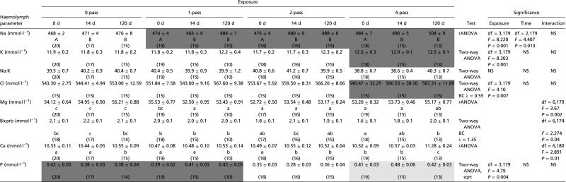All values are expressed as means ± SEM, with sample sizes indicated in parentheses. Information regarding the statistical test used [two-way ANOVA or randomized permutation test ANOVA (rANOVA)], along with identification of any transformation applied to data (BC λ, Box−Cox transformation with value for lambda indicated; sqrt, square root transformation) is provided. If exposure, sample time or the interaction between exposure and sample time were found to be a significant factor, the statistics and P values for that factor are given. NS, not significant. A and B indicate values for which sample time was a factor that was significantly different for any values not sharing an A or B, respectively. a, b, c, and d indicate a value for which the interaction between exposure and sample time was significantly different from any value not sharing an a, b, c, or d, respectively. White, light gray, and dark gray cells represent values for which exposure was a factor that was significantly different from any cells that were not white, light gray, or dark gray, respectively. Bicarb, bicarbonate.

Hemolymph sodium (Na) concentration showed a significant response to both exposure [F(3,179) = 8.220, P < 0.001] and sample time [F(2,179) = 4.407, P = 0.014], but not the interaction of the terms [F(6,179) = 1.930, P = 0.078], with exposure resulting in increased Na concentrations. Sample time showed significantly lower Na concentrations in day 0 samples compared with day 14 and day 120 samples. Exposure level significantly affected potassium (K) concentrations [F(3,179) = 8.303, P < 0.001], with four-pass scallops showing significantly higher K levels than zero-pass, one-pass, and two-pass scallops. Although there were differences in Na and K, there was no significant difference in Na:K ratio, in response to either exposure [F(3,179) = 2.373, P = 0.072] or sample time [F(2,179) = 0.126, P = 0.88].

There was a significant interaction between exposure and sample time for hemolymph concentration of magnesium [F(6,179) = 3.668, P = 0.0018], which tended to show a reduction in exposed scallops relative to controls; bicarbonate [F(6,174) = 2.274, P = 0.039], which was reduced in response to higher levels of exposure in the short and medium term; and calcium [F(6,180) = 2.891, P = 0.010], which was elevated in exposed scallops.

Chloride ions (Cl) differed significantly as a result of exposure [F(3,179) = 4.1, P = 0.007], with four-pass scallops showing elevated levels of Cl compared with zero-pass, one-pass, and two-pass scallops.

Phosphorus levels differed significantly as a result of exposure [F(3,179) = 4.791, P = 0.003], although, in this case, two-pass scallops had phosphorus levels significantly lower than zero-, one-, and four-pass scallops.

Organic molecules (Table S4 for all mean values and statistics) showed a more limited response, with significant differences only in total protein and glucose levels. For protein, exposure and sample time displayed a significant interaction [F(6,178) = 2.579, P = 0.020], although no significant differences were found among relevant treatments and sample times following post hoc analysis. For glucose, exposure had a significant effect [F(3,180) = 5.37, P = 0.01), with zero-pass scallops showing higher glucose levels than one-pass and four-pass scallops.

Table S4.

Effect of seismic exposure on hemolymph organic molecules in scallops from the 2014, 150-in³ experiment, based on exposure level (0-pass, 1-pass, 2-pass, and 4-pass) and sample time (0 d, 14 d, and 120 d postexposure)

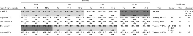All values are expressed as means ± SEM with sample sizes indicated in parentheses. Information regarding the statistical test used [two-way ANOVA or randomized permutation test ANOVA (rANOVA)], along with identification of any transformation applied to data (BC λ, Box–Box transformation with value for lambda indicated; sqrt, square root transformation) is provided. If exposure, sample time or the interaction between exposure and sample time were found to be a significant factor, the statistics and P values for that factor are given. White, light gray, and dark gray cells represent values for which exposure was a factor that was significantly different from any cells that were not white, light gray, or dark gray, respectively. Chol, cholesterol; Gluc, glucose; NS, not significant; TP, total protein; Trig, triglyceride; Uric, uric acid.

Discussion

A common criticism of animal exposure experiments with air gun sources is that they do not represent “real” seismic sources or that the exposure either exceeds or is lower than that of a “real” seismic source. In the present study, a single air gun was used in open-water, field conditions to expose scallops in a natural habitat setting to signals emulating a larger commercial seismic array. With an exposure regime based on multiple passes, scallops received SELs and ground excitation comparable to that of a large commercial source passing within a few hundred meters, based on comparisons with commercial arrays and modeling of multiple passes of commercial sources (33).

Here we found that seismic exposure, particularly repeated exposure, significantly increased mortality in the scallop P. fumatus compared with the 4 to 5% mortality rate in control scallops. The observed mortality rates in all three experiments, which ranged from 9 to 11% in one-pass scallops to 13 to 20% in four-pass scallops, were not representative of a mass mortality event (34) and were at the low end of the range of the naturally occurring mortality rate documented in the wild, which ranges from 11 to 51% with a 6-y mean of 38% and a well-established correlation to fishery stress (35–37). However, given the arbitrary endpoint of 120 d postexposure, mortality could have potentially continued to increase in the exposed treatments.

One way in which seismic air gun exposure could result in mass mortality is by driving scallops to energetically expensive behaviors such as extensive swimming or long periods of valve closure, although neither qualitative analysis of behavior during exposure nor quantitative analysis of tentacle state (38, 39) offered support for this hypothesis. However, exposed scallops showed two disruptions to behavioral patterns. First, exposed scallops demonstrated a marked reduction in classic behaviors during exposure. Second, exposed scallops exhibited a novel velar flinch behavior. This novel flinching behavior was only observed in direct response to air gun signals, often slightly before the signal was audible, suggesting that the behavior is in response to the faster-traveling groundborne energy. Whether these changes in behavior might have an ecological impact on scallops is not clear. The velar flinch cannot be interpreted as a sign of stress or negative impact on its own, although it is clearly an acute response to exposure. The reduction in classic behaviors, potentially an indication of a reduced capacity to respond to other stimuli, was apparent only during exposure. As there was no difference in behavior between control and exposed scallops in the postexposure observation period, any long-term manifestation of this behavioral response is unlikely.

The scallops’ recessing reflex, in which a scallop uses jets of water to create a depression in the sediment while also covering itself with sediment, was also impacted by exposure. Recessing appears to be the “natural” state for scallops in the Pecten genus (28, 29), assisting feeding, conferring protection from predators, preventing shell fouling, and reducing hydrodynamic profile (40). Typically, scallops demonstrate slowed recessing in response to stress, resulting from energy depletion during exposure (40–42); however, seismic exposure elicited the opposite effect, with repeated exposure increasing the rate of recessing. Furthermore, in these previous studies, the recessing time in stress-affected scallops had returned to normal within 1 d to 3 d (40–42), whereas, in the present study, the impacted response persisted to at least 120 d after exposure. Given that energy depletion caused the slowed recessing previously observed, it is not surprising that scallops exposed to air gun signals did not respond similarly, as swimming or valve closing behavior was not observed during air gun exposure. However, the more rapid recessing of exposed scallops cannot easily be explained.

We hypothesize that exposure impacted elements of the scallop sensory system, with the statocyst and the abdominal sense organ as potential candidates. The paired statocysts are the primary mechanosensory organ in scallops, as in many invertebrates, that provide a sense of balance through reception of gravity (43). The abdominal sense organ, a sickle-shaped pocket in the mantle fold densely populated with sensory hairs, has been indicated to play a role in mechanoreception and directional sensitivity (44), based on its high sensitivity to water- and ground-borne vibrations (45, 46). If the abnormal reflex results found in this study are indicative of damage to mechanosensory organs, exposed scallops may face considerable ecological ramifications. Disruption of the statocyst nerve caused scallops to lose the ability to control the vertical component of their swimming (47), thus compromising a primary mechanism of predator avoidance. The abdominal sense organ has also been suggested to contribute to predator detection, with the detection of waterborne vibrations originating from above the scallop filling in a blind spot of the visual, tactile, and chemoreceptive systems (48).

The physiological response to exposure was explored through the hemolymph of the scallop, which is the invertebrate analog to vertebrate blood and performs many of the same functions, including gas exchange, nutrient and waste transport, osmoregulation, and immune function (45). Although these hemolymph parameters are useful for interpreting health, care must be taken in comparisons over time, as bivalve hemolymph tends to show considerable variation in hemolymph parameters in response to biotic (reproductive cycle, nutritional condition) and abiotic (temperature, food availability) factors (30, 49–51). This variability is particularly relevant to the 2015 experiment in this study, which was conducted in the summer, whereas the 2013 and 2014 experiments were conducted in the winter. This seasonal difference, along with having only one sampling point in the 2015 experiment, makes comparing the 2015 experiment to the winter experiments difficult, due to the influence of water temperature, nutritional condition, and reproductive state.

The effect of exposure on the cellular component of the hemolymph, which is responsible for mediating immune function, was quantified through total hemocyte counts. We found that our hypothesis regarding hemocyte counts, that exposure would cause a short-lived increase in the number of circulating hemocytes in a response similar to that of other stressors, was largely unsupported. In 2013, scallops had comparatively low hemocyte levels early in the experiment (i.e., days 0 and 14), with exposed treatments receiving multiple passes showing depressed hemocyte counts compared with controls. Conversely, in 2014, exposed scallops showed elevated hemocyte numbers at day 14 compared with controls, consistent with the typical bivalve response to stress (30). The dissimilarities between experiments in hemocyte response at initial sample points can likely be attributed to the differences in collection methods, as scallops for the 2013 experiment were collected via dredging and scallops for the 2014 and 2015 experiments were hand-collected by divers. The response to exposure of the 2013 scallops probably includes a latent response to the stresses resulting from dredging and repeated transportation (41), with the comparatively low levels of hemocytes and the immediate hemocyte response observed in exposed scallops in the 2013 experiment suggesting a synergy between dredging stress and seismic exposure that accelerated the overall response.

In both the 2013 and 2014 experiments, hemocyte numbers had decreased by day 120 in exposed scallops. Although conclusions regarding immune function cannot be directly drawn from hemocyte count results, the depressed levels in exposed scallops suggest that the scallops in this study were immunocompromised, one of the most important drivers of mortality in bivalves (52, 53), and direct assays of immune function (i.e., differential hemocyte counts; assays of phagocytosis, hemocyte membrane stability, etc.) are an important next step for understanding the impacts of exposure.

Like hemocyte counts, hemolymph pH indicated that the scallops in the 2013 experiment showed stress from dredging. In that experiment, hemolymph pH values were high at days 0 and 14 in control and all exposed treatments compared with those from the subsequent experiments, with levels of >8.00 and >7.85, respectively. By day 120 postexposure, pH levels in all treatments, including controls, had returned to the expected range (between 7.46 and 7.63), with no difference between any treatments. These results followed our hypothesis of stable hemolymph biochemistry; however, the stress response would have masked any experimental response. In the 2014 and 2015 experiments, the prediction of stable pH was unsupported, as exposure resulted in elevated pH levels, or alkalosis. Reports of alkalosis in marine invertebrates are rare in the literature. The only report of alkalosis in a marine bivalve, the Pacific oyster Crassostrea gigas (54), resulted from extensive handling, shell drilling, cannulation, and repeated drawing of hemolymph. More broadly, alkalosis in marine invertebrates, primarily cephalopods, has been reported to occur in response to functional and environmental hypoxia as metabolism shifts to anaerobic pathways (55–60). There are considerable differences between these reported cases of alkalosis and its occurrence observed here. In the present study, scallops were in normoxic seawater throughout the experiment and demonstrated a decrease in hemolymph bicarbonate, rather than the increase typical of other molluscs, suggesting that mobilization of bicarbonate from the shell is unlikely to be a factor in the response. Furthermore, alkalosis in scallops was persistent for at least 14 d, far longer than the scale of hours previously reported in any invertebrate. The mechanisms of this response warrant further study, as they likely differ from those previously investigated, given the substantially different circumstances between this study and previous reports of alkalosis.

Exposure to air gun signals also resulted in considerable and persistent osmoregulation disruption, as the a priori hypothesis of stable hemolymph biochemistry was again unsupported. Owing to adaptation to the stable nature of their sublittoral habitat, scallops show a limited capacity for regulation of hemolymph ion concentration (61, 62). However, a broad scope of changes was observed, with every mineral and electrolyte assayed showing a significant alteration in response to exposure. Changes in hemolymph ion concentration have been observed in abalone (Haliotis diversicolor supertexta) in response to osmotic stress (63) and hypoxia (64), but not in response to thermal stress (65). It is notable that hemolymph electrolyte ions in stressed abalone stabilized within days, whereas the scallops in the present study showed changes over chronic time scales. Cellular damage decreased hemolymph sodium and chloride concentration and increased potassium concentration in mussels (Mytilus edulis) in response to the interaction of anoxia, metal toxicity, temperature, and salinity (66). It is difficult to conclude whether cellular damage played a role in the scallops’ response to exposure, as damage causing cellular leakage would be expected to increase the hemolymph concentration of all hypotonic cellular ions. However, although some hypotonic ions (e.g., potassium) increased as would be expected, others (e.g., magnesium) decreased following exposure. Whatever the mechanism, these imbalances in hemolymph electrolyte ions can disrupt the membrane potential, affecting a range of biological functions, such as proton pump function, active transport across the cell membrane, and enzyme function within the cell (66).

Exploration for petroleum and the development of shellfish fisheries are necessary processes for these extractive industries that need to coexist in the marine environment. In this study, exposure to seismic surveys left scallops behaviorally and physiologically impacted and in a state such that any additional stress (e.g., dredging, warm water conditions, predation stress) could lead to further impairment or mortality (67). These results indicate a need for further study into the impacts of seismic signals, and, more generally, anthropogenic aquatic noise. In all cases, the mechanistic underpinnings and ecological impacts of these responses to exposure require further characterization to understand the overall economic and ecological implications. To avoid future conflict, a comprehensive understanding of how these industries may impact each other will be required in order to facilitate effective management.

Methods

Animal Care and Experimental Design.

The present study comprised three experiments exposing the commercial scallop (P. fumatus) to signals from a Sercel G Gun II operated at 2,000 psi. The first experiment, referred to as the 2013 experiment hereafter, was conducted in July 2013 (austral winter) using 240 adult scallops that were collected by a commercial scallop dredge fishing vessel from the fishery near Ille des Phoques, Tasmania (42°21’20.62”S 148°10’3.25”E; Fig. 4). For this experiment, the air gun was fitted with a 45-in³ chamber for exposure. Scallops were randomly assigned to four treatments of exposure levels defined by the number of passes of the seismic air gun—zero passes (control), one pass, two passes, and four passes—and color-coded and numbered tags (Glue On Shellfish Tags; Hallprint Fish Tags) were used to identify the treatment and individual. To determine whether time was a factor in any observed response, scallops from each of these treatments were sampled at three different points following exposure: 0 d, 14 d, and 120 d. Thus, 12 scallops (i.e., three sample days × four treatment levels) were placed into each of the 20 enclosures at the field site.

Fig. 4.

Scallop experiment locations: 1, IMAS; 2, Blackjack Rocks, field site; 3, Spring Bay Seafoods, Triabunna, mussel lease where day 120 scallops were held; 4, Ille de Phoques, collection site for 2013, 45-in³ experiment; and 5, Coles Bay, collection site for 2014 and 2015, 150-in³ experiments. Map data obtained from Google Earth.

For the second experiment, referred to as the 2014 experiment hereafter, was conducted in July 2014 (austral winter) using a 150-in³ chamber on the air gun, and 240 adult scallops were hand-collected by divers from Coles Bay, Tasmania (42°07’45.07”S, 148°16’03.83”E; Fig. 4). Treatment groups and sample times were identical to those of the 2013 experiment.

The final experiment, the 2015 experiment, was conducted in March 2015 (austral summer), again using a 150-in³ chamber on the air gun. For this experiment, the number of treatment groups was reduced to two (zero-pass and four-pass) and the number of sample points was reduced to two (14 d, 120 d), so 80 adult scallops were used. Scallops were again hand-collected by divers from Coles Bay, Tasmania, at the same site as the 2014 experiment, with four scallops (i.e., two sample days × two treatment levels) placed into each enclosure.

Before and following experimental field work, scallops used in this study were held at the Institute for Marine and Antarctic Studies (IMAS), Taroona, Tasmania (42° 56’59.13”S, 147° 21’16.60” E; Fig. 4), in a 3,400-L (2 m × 2 m × 0.85 m) tank with ca. 10 cm of sand substrate with ambient temperature (ca. 13 °C in 2013 and 2014 experiments, ca. 17 °C in 2015 experiment) seawater supplied by a flow-through system. Scallops were held at IMAS for 1 wk before transport to the field site. Scallops were transported to IMAS in plastic bins lined and covered with burlap sacks wetted with seawater (68).

The field site for all three experiments, near Blackjack Rocks north of Betsey Island, Tasmania (43°02’16.37”S, 147°28’30.14”E; Fig. 4), was a sand flat at 10 m to 12 m depth. Scallops were transported to the site in a large bin (1.2 m × 0.75 m × 1 m) of seawater. A deck hose was used to pump fresh seawater into the bin to maintain O₂ levels. At the field site, divers placed scallops into 1.5-m-tall cylindrical enclosures (Fig. S3) constructed of 2-cm mesh with a 1.2-m-diameter floating ring at the top and skirted by a ring of heavy-gauge chain at the bottom. Enclosure bottoms were not meshed, allowing for scallops to be in contact with the sandy seabed. Scallops were held in the enclosures for a 2-d acclimation period before the experiment.

Fig. S3.

Photograph of scallop enclosure in situ at field site. Enclosures had a float ring at the top and a chain ring skirting the bottom to keep the enclosure aloft in the water column, with parallel lines of rope used to secure enclosures in case of rough conditions. The bottom was unmeshed to allow scallops contact with the substrate.

In the 2014 and 2015 experiments, video cameras were placed into 10 randomly selected scallop enclosures at the start of the experiment to allow for behavioral analysis of scallops during the control pass and before, during, and following each air gun exposure pass.

All research was conducted in accordance with University of Tasmania Animal Ethics Committee Permit A13328. Fieldwork was conducted in accordance with Tasmania Department of Primary Industries, Parks, Water and Environment Permits 13011 and 14038.

Exposure and Air Gun Measurements.

At the beginning of the experimental procedure, the air gun vessel was positioned ∼1 km from the scallop enclosures, with the air gun deployed and towed at a depth of 5.1 m. First, a control (zero-pass) run was conducted, in which the air gun was deployed and charged but not fired. The vessel approached the scallop enclosures at a speed of 1.85 m⋅s⁻¹ (3.5 kn) following a predetermined path that was used for all runs (Fig. S4). Following the control run, divers collected the scallops assigned to the control treatment based on tag color. Upon retrieval, scallops were randomly assigned to sample points (0 d, 14 d, or 120 d postexposure in 2013 and 2014; 14 d or 120 d postexposure in 2015) and placed into a large bin of seawater continually supplied with fresh seawater via the deck hose. After zero-pass control scallops were collected, the air gun vessel returned to the starting point and began firing the air gun, with one shot every 11.6s, while following the approach toward the scallop enclosures. At the conclusion of the run, divers collected the scallops assigned to the one-pass treatment, which were assigned to sample times and placed into the bin of seawater and returned to IMAS. The same process was followed for passes two through four. Following each air gun pass, the air cylinders used to power the air gun required recharging via onboard scuba compressors. As this process lasted for several hours, the number of air gun runs that could be conducted was limited, so the zero-pass and one-pass runs were conducted in 1 d and passes two through four were conducted the following day.

Fig. S4.

Layout of the three scallop experiments at a small scale (Top) and large scale (Bottom) for (A) 2013 experiment, (B) 2014 experiment, and (C) 2015 experiment, with the cages shown by the dots (during experiment 1, the cages were colocated with sea noise recorders); the sea noise logger locations shown by the black squares; air guns shown by blue (run 1), black (run 2), red (run 3), and magenta (run 4), with individual air gun shot locations given by the cross along the respective line; and the 2014 and 2015 control runs shown in green. (Top) The numbers are the sea noise logger set number. Shown is the cage layout with the grid scale in meters and the axis arbitrarily scaled to the approximate center of the line of pots. (Bottom) The bathymetry contours are from the coast: 5 m, 10 m, 15 m, and 20 m.

Upon return to IMAS, day 0 scallops were placed into a plastic crate that remained immersed in the holding tank. Scallops were haphazardly selected from this crate for sampling, until all were done. Scallops not sampled on day 0 were used in recessing tests (details in Sampling). Following the recessing test, day 14 scallops were held at IMAS, whereas day 120 scallops were haphazardly distributed into two lantern nets. The nets were placed into bins lined and covered with burlap sacks wetted with seawater and transported to Spring Bay Seafoods in Triabunna, Tasmania (42°35’59.65”S, 148°01’01.83”E; Fig. 4), where the lantern nets were deployed on mussel aquaculture lines that were held submerged at a depth of 10 m. The nets were left undisturbed until they were recovered and returned to the holding tanks at IMAS 1 wk before sampling at day 120, to allow for acclimation following transport.

Hydrophones placed on the seabed monitored the normal ambient noise and the air gun signals (sound pressure) received by the scallops, and geophones were placed to measure groundborne vibrations (velocity) before and during the experiment. Sea noise loggers were located next to scallop enclosures at each end of the scallop lines. A near-field logger was also deployed 0.5 m off the air gun ports to allow source levels to be quantified. A detailed description of the methods used to determine sound levels is given in Supporting Information.

To determine how the exposure regimes in this experiment equated to exposure to full-scale seismic surveys, measured levels were compared with those of a modeled 3,065-in³ 3D array source operating in 50-m water depth, based on data collected from previous surveys (1, 33). Additional details of this model are provided in Supporting Information.

Sampling.

Mortality was assessed throughout the postexposure holding period through observation of abnormal positioning (i.e., inverted on the substrate, not recessed for an extended period, leaned up against the side of the tank, etc.) during periodic (i.e., at least three times per week) monitoring of the scallop tank or through discovery during sampling. Any observed mortalities were rounded to the next sampling point, i.e., a dead scallop discovered at day 10 was considered dead at the day 14 sample point. For the day 120 scallops, once scallops were transported to the mussel lease, mortality was not assessed until the scallops were returned to IMAS before sampling. Mortality rate was determined by comparing the total number of dead scallops from each treatment. Only mortalities observed following recovery were considered; that is, losses due to predation or unrecovered animals were not counted in the analysis.

Video recordings made during seismic exposure in the 2014 and 2015 experiments were used to analyze scallop behavior. Recordings were divided into three categories: preexposure, intraexposure, and postexposure segments, with the first 5 mins of preexposure time and the last 5 mins of postexposure time disregarded due to the influence of divers deploying and retrieving video cameras. For each segment, all visible scallops were observed and two sets of behavioral data were recorded. First, the observed behaviors were classified into two categories, classic and nonclassic, with the former encompassing visual behaviors, e.g., reflexive closure response to shadow or movement; “coughs” used to irrigate the mantle cavity; valve closures characterized by mantle velum retraction and valve adduction; and locomotory behaviors, such as swimming or repositioning (69). Any behaviors not encompassed within the classic behavior category were classified as nonclassic. The second analyzed behavior was tentacle extension, which was used as a method to evaluate valve closure (39), with tentacles recorded as either “extended,” “partially extended,” or “retracted” for the duration of the preexposure, intraexposure, and postexposure time categories for the 2014 and 2015 experiments. Extended and partially extended tentacles were considered to indicate that valves were open, and tentacle retraction indicated valve closure. It is important to note that the preexposure periods differ somewhat between the one-pass treatment and the higher exposure treatments, in that the one-pass scallops were naïve to any air gun exposure during the preexposure period, whereas two- and four-pass scallops had been exposed during the intraexposure period of the previous treatments.

At each of the three sample points (at days 0, 14, and 120 postexposure in the 2013 and 2014 experiments and at day 14 in the 2015 experiment), all individuals within the four treatment levels (two treatment levels in the 2015 experiment) were terminally sampled. First, the adductor muscle was detached from the upper valve, and then the upper valve was removed. Then, 2.5 mL of hemolymph was drawn from each scallop from the pericardial sinus using a prechilled syringe fitted with a 26-gauge needle. This sample was divided into two aliquots: a 500-μL aliquot for immediate analysis of pH (Testo 205 pH meter) and a 500-μL aliquot that was added to a centrifuge tube prefilled with 500 μL of anticoagulant (Lillie's formol calcium: 2% NaCl, 1% calcium acetate, 4% formaldehyde) for total hemocyte counts using an improved Neubauer hemocytometer under 40× magnification. In the 2014 experiment, an additional 1,500-μL aliquot was drawn and centrifuged at 3,000 × g for 3 min, after which 1,000 μL of supernatant was transferred into a cryovial and snap-frozen in liquid nitrogen for later biochemical analysis. This sample was shipped, frozen on dry ice, to Diagnostic Services at the Atlantic Veterinary College, University of Prince Edward Island, and analyzed using a Cobas c501 automated biochemistry analyzer (Roche Diagnostics Corporation) for a full blood profile consisting of the electrolytes (millimoles per liter = millimolars) sodium (Na), chloride (Cl), potassium (K), magnesium (Mg), and bicarbonate (bicarb); minerals (millimoles per liter) calcium (Ca) and phosphorus (P); metabolites (millimoles per liter = millimolars) glucose (Gluc), lactate (Lact), cholesterol (Chol), triglyceride (Trig), total protein (TP, in grams per liter) and uric acid (Uric, in micromoles per liter).

Beginning at day 0 upon return to IMAS following exposure, the scallops scheduled for destructive sampling at days 14 and 120 postexposure were used for a recessing reflex test (41, 42). Starting from when the scallops were placed into the holding tank following exposure, scallops were visually assessed for recessing three to four times daily at ∼6-h intervals, with recessing defined as having an upper valve even with the substrate level. To ensure consistent assessment of recessing, the same researcher performed all assessments. Once a scallop was observed to have recessed into the substrate, it was collected, and the time taken to recess (in hours) was recorded. In all three experiments, the recessing test continued until all scallops had recessed, which was under 5 d in all cases. In the 2014 experiment, this test was also conducted a second time, before the day 120 sample point using scallops scheduled for destructive sampling at day 120 postexposure.

Final sample sizes for each component of the three experiments at each sample point, which exhibited some variation due to differences in mortality rates and animals lost to predation or missing tags, are given in Table S5.

Table S5.

Sample sizes from each component of the scallop experiments

Sample time	Mortality, total hemocyte counts, pH, refractive index					Recessing				Hemolymph biochemistry assays
	0-pass	1-pass	2-pass	4-pass	0-pass	1-pass	2-pass	4-pass	0-pass	1-pass	2-pass	4-pass
2013
Day 0	16	19	17	20
Day 14	16	17	20	19	32	32	34	33
Day 120	17	15	16	14
2014
Day 0	20	19	17	19					20	19	18	18
Day 14	17	16	15	16	38	33	37	38	17	15	16	15
Day 120	16	12	15	12	16	12	15	12	15	15	15	15
2015
Day 14	19			17	32			33
Day 120	DOR	DOR	DOR	DOR	DOR	DOR	DOR	DOR

Blank cells indicate that no scallops were sampled for that parameter in the corresponding experiment. DOR, all scallops were dead on recovery.

Statistics.

To evaluate cumulative mortality in the 2013 and 2014 experiments, mortalities from each treatment were compared using a binomial regression. The analysis was restricted to the 2013 and 2014 experiments, as all scallops died while deployed on the mussel lease before the day 120 sampling point for both zero- and four-pass treatments in the 2015 experiment.

Comparisons of behavioral analysis were conducted on the rate (incidences per unit time) of observations of classic and nonclassic behaviors. Rates were used, as the observational period differed between the scallops, thereby complicating the use of conventional count-based models. Nonclassic behavior was only observed in exposed scallops; hence the nonclassic and classic behavioral modes were analyzed separately using a generalized linear model with the number of exposure passes, the year, and temporal category (preexposure, intraexposure, and postexposure) as categorical explanatory variables.

Tentacle extension was compared for each treatment by summing the duration each individual scallop spent in each of the three states of tentacle extension. This sum was then converted into a proportion of total time of each temporal category, and multinomial regression was used to analyze the behavioral modes (two options, since the proportions add up to 1) as a function of the year, treatment, and phase.

Recessing reflex data from all three experiments was analyzed using Kaplan−Meier estimator analysis of the time-to-recess for each individual and compared using log-rank (Mantel−Cox) test with α = 0.05, followed by multiple comparisons with Bonferroni correction and a family-wise error rate of 0.05.

Hemocyte count data from the 2013 and 2014 experiments were tested for assumptions of equality of variance (Levene’s test) and normality (Shapiro−Wilk test) before analysis using two-way ANOVAs with air gun passes and sample time as factors and α = 0.05, followed by a Tukey honest significant difference (HSD) post hoc test for significant results. Data from 2013 required log transformation, and data from 2014 required square root transformation. Data from the 2015 experiment were compared using a Welch Two-Sample t test between zero- and four-pass treatments at the 14-d sample point.

Hemolymph pH data for the 2013 experiment did not meet normality assumptions, so a two-way randomized permutation test ANOVA (70) with 5,000 iterations was used, with passes and sample time as factors and α = 0.05, followed by post hoc Tukey HSD tests for any significant results. For the 2014 experiment, data met ANOVA assumptions, so a two-way ANOVA with passes and sample time as factors and α = 0.05 was used. Significant results were analyzed using a Tukey HSD post hoc test. For the 2015 experiment, pH was compared using a Welch t test between zero- and four-pass treatments at the 14-d sample point.

Biochemistry data from the 2014 experiment was analyzed using two-way ANOVA for parametric data and randomized permutation test two-way ANOVA for nonparametric data, with passes and sample time as factors and α = 0.05, followed by post hoc using Tukey HSD tests to evaluate significant results.

Except where noted otherwise, all statistical comparisons were conducted using R v3.1.3 (The R Foundation for Statistical Computing).

SI Methods

Units and Air Gun Signal Analysis.

All times given here are Australian Eastern standard Time [EST = Universal Time Coordinated (UTC) + 10 h] or EST with daylight saving (UTC + 11 h). All times zones are indicated appropriately. All air gun and spatial analysis has been carried out in the Matlab (The Mathworks Inc.) environment using purpose-built software. Air gun signals were analyzed by (i) in a graphical user interface (GUI) designed to deal with air gun signal extraction, visualizing each high gain sea noise sample (spectrogram and waveform) with potential air gun signals, obtaining a voltage threshold which delineated air gun signals from the noise and setting the preexposure and postexposure time brackets around the detections (the time window to analyze the signal in); (ii) using the signal filtered to keep the waterborne energy (removing groundborne energy), locating the leading edge of each air gun signal using the voltage threshold set and a minimum time limit of how far apart consecutive signals must be (5 s used); (iii) checking the input voltage of each air gun signal for overloads and loading the low gain channel if an overload was found (the sea noise loggers are considered as overloaded if the voltage is >2.4 V or <−2.4 V); (iv) displaying the location of the waterborne arrival in the GUI and manually removing any false detections; (v) obtaining a time period to bracket the waterborne signal with—this was nominally set at ±3 s but altered if the air gun signal had leading or trailing energy which fell outside of this window; (vi) bracketing the identified air gun signal time window using a multiple of two points, extracting the signal and calibrating to pascals in the time domain, accounting for variation in the system gain with frequency and using the system hydrophone sensitivity for the appropriate channel (see below)—this step gave the calibrated air gun signal waveform in pascals; (vii) calculating a suite of signal descriptors (41) plus identifying the time of air gun signal waterborne arrival; (viii) calculating the power spectra of each sample (as close as possible to a 1-Hz bandwidth used); and (ix) looping through all identified air gun signals and saving the signal descriptors, received times, power spectra, and the calibrated air gun waveform.

Each air gun signal was calibrated from volts to pascals by extracting the noise logger signal bracketing the identified air gun signal in a multiple of two points, which was greater than the identified signal length, and passing this to a program which (i) returned the fast Fourier transform (FFT) of the input waveform section (multiple of two points) at a frequency resolution of close to 0.1 Hz; (ii) calculated the system gain in linear units at a frequency spacing the same as given by the above FFT step, from 0 Hz to the Nyquist frequency, this gain including the hydrophone sensitivity; (iii) applied the linear gain correction to the FFT amplitude; (iv) assumed a unity phase correction applied to the FFT phase; (v) inverted the FFT back into the time domain; and (vi) extracted the required air gun signal (since it was of shorter duration than the section calibrated) from this corrected section of the waveform.

The analysis gave the air gun signal descriptors, power spectra, received arrival time of signals (logger clock corrected for drift), and the signal waveform. The time of each received air gun signal was then used to extract spatial information of the receiver location relative to the source. This involved (i) using the received shot time at the sea noise logger (waterborne arrival) to locate the closest shot in the air gun track file, then iterating the time/range of this and the previous few shots, allowing for signal travel time, to find the fired shot point which best matched the fired time plus estimated travel time to give the sea noise logger received time; (ii) for the identified air gun fired location, calculating the receiver range (horizontal and slant range), the air gun speed and heading, and the take-off angle of the receiver to the air gun heading (i.e., angle of the receiver from the air gun heading); and (iii) saving all data.

All data were saved in a standard format. Of the 16 signal parameters, saved peak pressures, rms pressure, SEL, and signal duration were pertinent here. The signal duration was defined as the time taken for 90% of the signal energy to pass, with the time at which 5% and 95% of the signal energy reached defining the air gun signal onset and end (72).

The geophone data were extracted from the noise loggers using the time bounds defined for the appropriate noise logger air gun waterborne signal. A linear calibration was assumed and applied to correct the saved volts to velocity (meters per second), according to the system gain used (0 dB or 20 dB) and the specifications of the particular geophone. The geophone response had been checked and found to match the manufacturer’s specifications. The geophones gave two horizontal (90° to each other) and one vertical velocity. The respective velocities were differentiated to give acceleration (meters per second squared) in the vertical or the vector sum in the horizontal. For analysis, here the absolute magnitude of the three-component acceleration vector has been used, and termed ground roll acceleration. This was calculated using a Matlab vector function (cart2pol.m). The acceleration magnitude has been expressed throughout in linear terms (meters per second squared) or to show trends with range, in decibel terms relative to 1 m⋅s⁻² [i.e., dB re 1 m⋅s⁻² as 10*log₁₀(LinearValue/1)].

Comparative Commercial Seismic Exposures.

A common criticism of animal exposure experiments with air gun sources is that they do not represent “real” seismic sources or that the exposure exceeds or is lower than that for a “real” seismic source. To address this, we have generated a simple model of air gun exposure from a “real” seismic source, for comparison with experimental exposures.

Data of the “real” seismic source (1, 41, 42, 69) were used to model a seismic source operating according to the following parameters: (i) a 3,065-in³ source operating in 3D mode; (ii) two sources operated alternatively, each source located centrally 50 m either side of the sail line; (iii) four streamers spaced 100 m apart and symmetric about the sail line (a 300-m spread between outermost streamers); (iv) a 25-m along-sail-line, signal spacing; (v) a 400-m sail-line spacing; (vi) 50 m water depth; (vii) two lines sailed adjacent to the chosen sail line; (viii) an east−west orientation; and (ix) a 2-km grid about the central receiver location (point [0 0]).

The water depth was chosen to be representative of that from an area commonly fished for scallops. Five sail lines were used, so statistics per line and the cumulative or maximum levels reached considering one or all lines were calculated. The geometry of a survey was modeled as one set of five sail lines with the central sail line directly over the receiver location (the sources were thus 50 m offset horizontally). Note that the air gun sources are each 50 m adjacent to the sail line, so maximum exposure is reached when a sail line has a 50-m offset from the receiver (always at [0 0]). The model was set up using empirical fits given below and run with a series of sail-line offsets.

To model received levels, empirical curves of transmission for SEL and maximum magnitude of ground roll were sourced for a large air gun array, as best as possible operating over sand in a similar water depth. From the seismic decay curves with range (33), we get a relationship of SEL with range using the mean of a 3,090- and a 3,040-in³ source operating over sand in 100 m to 150 m water depth (each source gave a correlation when using a curve of the form below of r² = 0.99 and r² = 0.95 with similar values for each constant), defined by

$$RL=\left[-23.33\ast {\log }_{10}\left(R\right)\right]+\left[-0.003\ast R\right]+234.8,$$

where RL is received SEL (dB re 1 µPa²·s), and R is slant range (direct range source to seabed receiver in meters). These values were considered to apply to a 3,065-in³ source. Note that this curve tracks the range-averaged trend for the given air gun arrays and thus removes air gun array directionality and sound transmission effects (69).

A relationship for the maximum magnitude of ground roll with range was derived using the same instruments as used here and a 3,130-in³ source operating in 40 m of water (69) as

$$G{R}_a=\left[-11.51*{\log }_{10}\left(R\right)\right]+\left[-0.0004*R\right]+36.9,$$

where GR_a is the maximum magnitude of ground roll in decibel values (dB re 1 m⋅s⁻²) for each air gun signal, and R is horizontal range (in meters). The measured data gave a correlation coefficient, using this fit, of r² = 0.85.

For comparison, the 150-in³ air gun measured here during the scallop experiments (45 in³ and 150 in³) gave a fitted curve for ground roll of

$$G{R}_b=\left[-6.88\ast {\log }_{10}\left(R\right)\right]+\left[-0.0021\ast R\right]+21.1,$$

where GR_b is the maximum magnitude of ground roll in decibel values (dB re 1 m⋅s⁻²) for each air gun signal, and R is horizontal range (in meters). The measured data gave a correlation coefficient, using this fit, of r² = 0.78.

Using these semiempirical fits and the geometry including five sail lines so as to estimate cumulative exposures of multiple passes, the curves for closest sail line and (i) estimated maximum magnitude of ground roll for any single signal (no cumulative effects considered for ground roll), (ii) the maximum SEL experienced along any line, and (iii) the cumulative SEL for all five lines are shown on Fig. S2. Note that, when the model was run with only one sail line, the cumulative SEL values shifted down by only a fraction of a decibel; thus the 2D seismic case is similar to that plotted on Fig. S2. The x axis given on Fig. S2 is for the closest sail line to the receiver location; thus the other four lines in the calculations would have been adjacent to this sail line and away from the receiver.

References

- 1. International Association of Geophysical Contractors & Oil and Gas Producers (2011) An Overview of Marine Seismic Operations (Int Assoc Geophys Contractors Oil Gas Producers, London), Rep 448.
- 2.Carroll A, et al. Environmental considerations for subseabed geological storage of CO2: A review. Cont Shelf Res. 2014;83:116–128. [Google Scholar]
- 3.Richardson WJ, Greene CR, Jr, Malme CI, Thomson DH. Marine Mammals and Noise. Academic; San Diego: 2013. [Google Scholar]
- 4.Popper AN, Hastings MC. The effects of human-generated sound on fish. Integr Zool. 2009;4:43–52. doi: 10.1111/j.1749-4877.2008.00134.x. [DOI] [PubMed] [Google Scholar]
- 5.Hawkins AD, Pembroke AE, Popper AN. Information gaps in understanding the effects of noise on fishes and invertebrates. Rev Fish Biol Fish. 2015;25:39–64. [Google Scholar]
- 6.Day RD, McCauley RD, Fitzgibbon QP, Semmens JM. Seismic air gun exposure during early-stage embryonic development does not negatively affect spiny lobster Jasus edwardsii larvae (Decapoda: Palinuridae) Sci Rep. 2016;6:22723. doi: 10.1038/srep22723. [DOI] [PMC free article] [PubMed] [Google Scholar]
- 7.Pearson WH, Skalski JR, Sulkin SD, Malme CI. Effects of seismic energy releases on the survival and development of zoeal larvae of Dungeness crab (Cancer magister) Mar Environ Res. 1994;38:93–113. [Google Scholar]
- 8.McCauley RD, Day RD, Swadling KM, Fitzgibbon QP, Semmens JM. Marine seismic survey air gun operations negatively impact zooplankton. Nat Ecol Evol. 2017;1:0195. doi: 10.1038/s41559-017-0195. [DOI] [PubMed] [Google Scholar]
- 9.Aguilar de Soto N, et al. Anthropogenic noise causes body malformations and delays development in marine larvae. Sci Rep. 2013;3:2831. doi: 10.1038/srep02831. [DOI] [PMC free article] [PubMed] [Google Scholar]
- 10.André M, et al. Low‐frequency sounds induce acoustic trauma in cephalopods. Front Ecol Environ. 2011;9:489–493. [Google Scholar]
- 11.Solé M, et al. Ultrastructural damage of Loligo vulgaris and Illex coindetii statocysts after low frequency sound exposure. PLoS One. 2013;8:e78825. doi: 10.1371/journal.pone.0078825. [DOI] [PMC free article] [PubMed] [Google Scholar]
- 12.Solé M, et al. Does exposure to noise from human activities compromise sensory information from cephalopod statocysts? Deep Sea Res Part II Top Stud Oceanogr. 2013;95:160–181. [Google Scholar]
- 13.Popper AN, Fay RR. Sound detection and processing by fish: Critical review and major research questions. Brain Behav Evol. 1993;41:14–38. doi: 10.1159/000113821. [DOI] [PubMed] [Google Scholar]
- 14.Rogers PH, Hawkins AD, Popper AN, Fay RR, Gray MD. The Effects of Noise on Aquatic Life II. Springer; New York: 2016. Parvulescu revisited: Small tank acoustics for bioacousticians; pp. 933–941. [DOI] [PubMed] [Google Scholar]
- 15.Joll L. Swimming behaviour of the saucer scallop Amusium balloti (Mollusca: Pectinidae) Mar Biol. 1989;102:299–305. [Google Scholar]
- 16.Tremblay I, Guderley HE, Himmelman JH. Swimming away or clamming up: The use of phasic and tonic adductor muscles during escape responses varies with shell morphology in scallops. J Exp Biol. 2012;215:4131–4143. doi: 10.1242/jeb.075986. [DOI] [PubMed] [Google Scholar]
- 17.Newell RI. Ecosystem influences of natural and cultivated populations of suspension-feeding bivalve molluscs: A review. J Shellfish Res. 2004;23:51–62. [Google Scholar]
- 18.Food and Agriculture Organization of the United Nations . Fishery and Aquaculture Statistics Annual Yearbook 2014. Food Aquacult Org United Nations; Rome: 2016. World fishery production; pp. 48–50. [Google Scholar]
- 19.Food and Agriculture Organization of the United Nations . The State of the World Fisheries and Aquaculture 2016. Fisheries Aquacult Org United Nations; Rome: 2016. Fish utilization and processing; pp. 45–51. [Google Scholar]
- 20.Shumway SE, et al. Shellfish aquaculture—In praise of sustainable economies and environments. World Aquacult. 2003;34:8–10. [Google Scholar]
- 21.MacDonald BA, Robinson SM, Barrington KA. Feeding activity of mussels (Mytilus edulis) held in the field at an integrated multi-trophic aquaculture (IMTA) site (Salmo salar) and exposed to fish food in the laboratory. Aquaculture. 2011;314:244–251. [Google Scholar]
- 22.Arbo P, Thủy PTT. Use conflicts in marine ecosystem-based management—The case of oil versus fisheries. Ocean Coast Manage. 2016;122:77–86. [Google Scholar]
- 23.Butt N, et al. Conservation. Biodiversity risks from fossil fuel extraction. Science. 2013;342:425–426. doi: 10.1126/science.1237261. [DOI] [PubMed] [Google Scholar]
- 24.Breitzke M. Overview of seismic research activities in the Southern Ocean—Quantifying the environmental impact. Antarct Sci. 2014;26:80–92. [Google Scholar]
- 25.Heide-Jørgensen MP, Hansen RG, Westdal K, Reeves RR, Mosbech A. Narwhals and seismic exploration: Is seismic noise increasing the risk of ice entrapments? Biol Conserv. 2013;158:50–54. [Google Scholar]
- 26.Dame RF. Ecology of Marine Bivalves: An Ecosystem Approach. 2nd Ed. CRC; Boca Raton, FL: 2011. Physical environmental interactions; pp. 43–62. [Google Scholar]
- 27.Hutson KS, Ross DJ, Day RW, Ahern JJ. Australian scallops do not recognise the introduced predatory seastar Asterias amurensis. Mar Ecol Prog Ser. 2005;298:305–309. [Google Scholar]
- 28.Baird R. On the swimming behaviour of escallops (Pecten maximus L.) J Molluscan Stud. 1958;33:67–71. [Google Scholar]
- 29.Minchin D. Introductions: Some biological and ecological characteristics of scallops. Aquat Living Resour. 2003;16:521–532. [Google Scholar]
- 30.Pipe RK, Coles JA. Environmental contaminants influencing immunefunction in marine bivalve molluscs. Fish Shellfish Immunol. 1995;5:581–595. [Google Scholar]
- 31.Hannam ML, Bamber SD, Galloway TS, John Moody A, Jones MB. Effects of the model PAH phenanthrene on immune function and oxidative stress in the haemolymph of the temperate scallop Pecten maximus. Chemosphere. 2010;78:779–784. doi: 10.1016/j.chemosphere.2009.12.049. [DOI] [PubMed] [Google Scholar]
- 32.Hannam ML, Bamber SD, Moody AJ, Galloway TS, Jones MB. Immunotoxicity and oxidative stress in the Arctic scallop Chlamys islandica: Effects of acute oil exposure. Ecotoxicol Environ Saf. 2010;73:1440–1448. doi: 10.1016/j.ecoenv.2010.06.012. [DOI] [PubMed] [Google Scholar]
- 33.McCauley RD, Duncan AJ, Gavrilov AN, Cato DH. Transmission of marine seismic survey, air gun array signals in Australian waters. In: Hillock IDM, Mee DJ, editors. Proceedings of ACOUSTICS 2016. Acoust Australia; Brisbane, QLD, Australia: 2016. [Google Scholar]
- 34.Sindermann CJ. Ocean Pollution: Effects on Living Resources and Humans. CRC; Boca Raton, FL: 1995. Mass mortalities in the sea: Natural and pollution-induced; pp. 113–126. [Google Scholar]
- 35.Coleman N, Gwyther D. 1988. Abundance of Scallops in Port Phillip Bay and Predictions of Yields for the 1988 Season (Mar Sci Lab, Queenscliff, VIC, Australia), Lab Tech Rep 67.
- 36.Medcof J, Bourne N. Causes of mortality of the sea scallop, Placopecten magellanicus. Proc Natl Shellfish Assoc. 1964;53:33–50. [Google Scholar]
- 37.Naidu K. Estimating mortality rates in the Iceland scallop, Chlamys islandica (O.F. Müller) J Shellfish Res. 1988;7:61–71. [Google Scholar]
- 38.Jonasson JP, Thorarinsdottir GG, Eiriksson H, Marteinsdottir G. Temperature tolerance of Iceland scallop, Chlamys islandica (O.F. Müller) under controlled experimental conditions. Aquacult Res. 2004;35:1405–1414. [Google Scholar]
- 39.Strand Ø, Solberg PT, Andersen KK, Magnesen T. Salinity tolerance of juvenile scallops (Pecten maximus L.) at low temperature. Aquaculture. 1993;115:169–179. [Google Scholar]
- 40.Maguire JA, O’connor DA, Burnell GM. An investigation into behavioural indicators of stress in juvenile scallops. Aquacult Int. 1999;7:169–177. [Google Scholar]
- 41.Maguire JA, Coleman A, Jenkins S, Burnell GM. Effects of dredging on undersized scallops. Fish Res. 2002;56:155–165. [Google Scholar]
- 42.Maguire JA, Jenkins S, Burnell GM. The effects of repeated dredging and speed of tow on undersized scallops. Fish Res. 2002;58:367–377. [Google Scholar]
- 43.Budelmann BU. Morphological diversity of equilibrium receptor systems in aquatic invertebrates. In: Atema J, Fay RR, Popper AN, Tavolga WN, editors. Sensory Biology of Aquatic Animals. Springer; New York: 1988. pp. 757–782. [Google Scholar]
- 44.Zhadan P, Semen’kov P. An electrophysiological study of the mechanoreceptory function of abdominal sense organ of the scallop Patinopecten yessoensis (Jay) Comp Biochem Physiol Part A Physiol. 1984;78:865–870. [Google Scholar]
- 45.Brand AR. Scallop ecology: Distributions and behaviour. In: Shumway SE, Parsons G, editors. Scallops: Biology, Ecology and Aquaculture. Elsevier; New York: 2006. pp. 651–744. [Google Scholar]
- 46.Zhadan PM, Sizov AV, Dautov SS. Ultrastructure of the abdominal sense organ of the scallop Mizuchopecten yessoensis (Jay) Cell Tissue Res. 2004;318:617–629. doi: 10.1007/s00441-004-0926-2. [DOI] [PubMed] [Google Scholar]
- 47.Buddenbrock W. Die statocyst von Pecten, ihre histologie und physiologie. Zool Jahrb Abt Anat Ontogenie Tiere. 1915;35:302–358. [Google Scholar]
- 48.Zhadan P. Directional sensitivity of the Japanese scallop Mizuhopecten yessoensis and Swift scallop Chlamys swifti to water-borne vibrations. Russ J Mar Biol. 2005;31:28–35. [Google Scholar]
- 49.Duchemin MB, Fournier M, Auffret M. Seasonal variations of immune parameters in diploid and triploid Pacific oysters, Crassostrea gigas (Thunberg) Aquaculture. 2007;264:73–81. [Google Scholar]
- 50.Lin T, et al. Seasonal variations of water temperature, food availability, size, and reproduction on the hemocyte parameters in the scallop Chlamys farreri. J Shellfish Res. 2012;31:663–670. [Google Scholar]
- 51.Thompson R. Blood chemistry, biochemical composition, and the annual reproductive cycle in the giant scallop, Placopecten magellanicus, from southeast Newfoundland. J Fish Board Canada. 1977;34:2089–2103. [Google Scholar]
- 52.Ford SE, Tripp M. 1996. Diseases and defense mechanisms. The Eastern Oyster Crassostrea virginica, eds Kennedy V, Newell RI, Eble A (Maryland Sea Grant Publ, College Park, MD), pp 467–513.
- 53.Shumway SE. 1996. Natural environmental factors. The Eastern Oyster Crassostrea virginica, eds Kennedy V, Newell RI, Eble A (Maryland Sea Grant Publ, College Park, MD), pp 467–513.
- 54.Jones TO, Bourne NF, Bower SM, Iwama GK. Effect of repeated sampling on haemolymph pH, PO2 and haemocyte activity in the Pacific oyster, Crassostrea gigas (Thunberg) J Exp Mar Biol Ecol. 1993;167:1–10. [Google Scholar]
- 55.Houlihan D, Innes A, Wells M, Wells J. Oxygen consumption and blood gases of Octopus vulgaris in hypoxic conditions. J Comp Physiol. 1982;148:35–40. [Google Scholar]
- 56.Pörtner HO, Webber DM, Boutilier RG, O’Dor RK. Acid-base regulation in exercising squid (Illex illecebrosus, Loligo pealei) Am J Physiol. 1991;261:R239–R246. doi: 10.1152/ajpregu.1991.261.1.R239. [DOI] [PubMed] [Google Scholar]
- 57.Pörtner H-O. Anaerobic metabolism and changes in acid-base status: Quantitative interrelationships and pH regulation in the marine worm Sipunculus nudus. J Exp Biol. 1987;131:89–105. [Google Scholar]
- 58.Pörtner H-O. An analysis of the effects of pH on oxygen binding by squid (Illex illecebrosus, Loligo pealei) haemocyanin. J Exp Biol. 1990;150:407–424. [Google Scholar]
- 59.Pörtner H-O, Grieshaber M, Heisler N. Anaerobiosis and acid-base status in marine invertebrates: Effect of environmental hypoxia on extracellular and intracellular pH in Sipunculus nudus L. J Comp Physiol B. 1984;155:13–20. [Google Scholar]
- 60.Seibel BA, et al. Metabolic suppression during protracted exposure to hypoxia in the jumbo squid, Dosidicus gigas, living in an oxygen minimum zone. J Exp Biol. 2014;217:2555–2568. doi: 10.1242/jeb.100487. [DOI] [PubMed] [Google Scholar]
- 61.Christophersen G, Strand Ø. Effect of reduced salinity on the great scallop (Pecten maximus) spat at two rearing temperatures. Aquaculture. 2003;215:79–92. [Google Scholar]
- 62.Wada K. Osmoregulation in marine bivalves. In: Sindermann CJ, editor. Proceedings of the Ninth and Tenth U.S.-Japan Meetings on Aquaculture. Natl Ocean Atmos Admin; Silver Spring, MD: 1984. pp. 89–92. [Google Scholar]
- 63.Cheng W, Yeh S-P, Wang C-S, Chen J-C. Osmotic and ionic changes in Taiwan abalone Haliotis diversicolor supertexta at different salinity levels. Aquaculture. 2002;203:349–357. [Google Scholar]
- 64.Cheng W, Liu C-H, Cheng S-Y, Chen J-C. Effect of dissolved oxygen on the acid–base balance and ion concentration of Taiwan abalone Haliotis diversicolor supertexta. Aquaculture. 2004;231:573–586. [Google Scholar]
- 65.Hooper C, et al. Effects of severe heat stress on immune function, biochemistry and histopathology in farmed Australian abalone (hybrid Haliotis laevigata × Haliotis rubra) Aquaculture. 2014;432:26–37. [Google Scholar]
- 66.Weber RE, de Zwaan A, Bang A. Interactive effects of ambient copper and anoxic, temperature and salinity stress on survival and hemolymph and muscle tissue osmotic effectors in Mytilus edulis. J Exp Mar Biol Ecol. 1992;159:135–156. [Google Scholar]
- 67.Burge CA, et al. Climate change influences on marine infectious diseases: Implications for management and society. Annu Rev Mar Sci. 2014;6:249–277. doi: 10.1146/annurev-marine-010213-135029. [DOI] [PubMed] [Google Scholar]
- 68.Peterson CH, Summerson HC, Luettich RA., Jr Response of bay scallops to spawner transplants: A test of recruitment limitation. Mar Ecol Prog Ser. 1996;132:93–107. [Google Scholar]
- 69.Wilkens LA. Neurobiology and behaviour of the scallop. In: Shumway SE, Parsons G, editors. Scallops: Biology, Ecology and Aquaculture. Elsevier; Oxford: 2006. pp. 123–227. [Google Scholar]
- 70.Manly BF. Randomization, Bootstrap and Monte Carlo Methods in Biology. CRC; Boca Raton, FL: 2006. [Google Scholar]
- 71.United States Geological Survey World Conventional Resources Assessment Team 2013 Supporting Data for the U.S. Geological Survey 2012 World Assessment of Undiscovered Oil and Gas Resources. U.S. Geological Survey Digital Data Series DDS-69-FF. Available at pubs.usgs.gov/dds/dds-069/dds-069-ff/. Accessed October 13, 2016.
- 72.McCauley RD, et al. Environmental Implications of Offshore Oil and Gas Development in Australia: Further Research. Australian Petroleum Production Exploration Association; Canberra, Australia: 2003. Marine seismic surveys: Analysis and propagation of air-gun signals; and effects of exposure on humpback whales, sea turtles, fishes and squid; pp. 364–521. [Google Scholar]
Associated Data
This section collects any data citations, data availability statements, or supplementary materials included in this article.