Extinction risk is most acute for the world’s largest and smallest vertebrates

Significance

Determining the drivers of extinction risk has been a key pursuit of conservation biology. Considering that body mass could be a strong predictor of extinction risk, we constructed a global database of body masses for 27,647 vertebrate species. Results show that the smallest- and largest-bodied vertebrates have elevated extinction risk. The largest vertebrates are mostly threatened by direct killing by humans, whereas the smallest species are more likely to have restricted geographic ranges—an important predictor of extinction risk—and be threatened by habitat degradation. Declines of large and small vertebrate species will truncate the size distributions characterizing these taxa, jeopardizing ecosystem services to humans, and generating cascading ecological and evolutionary effects on other species and processes.

Abstract

Extinction risk in vertebrates has been linked to large body size, but this putative relationship has only been explored for select taxa, with variable results. Using a newly assembled and taxonomically expansive database, we analyzed the relationships between extinction risk and body mass (27,647 species) and between extinction risk and range size (21,294 species) for vertebrates across six main classes. We found that the probability of being threatened was positively and significantly related to body mass for birds, cartilaginous fishes, and mammals. Bimodal relationships were evident for amphibians, reptiles, and bony fishes. Most importantly, a bimodal relationship was found across all vertebrates such that extinction risk changes around a body mass breakpoint of 0.035 kg, indicating that the lightest and heaviest vertebrates have elevated extinction risk. We also found range size to be an important predictor of the probability of being threatened, with strong negative relationships across nearly all taxa. A review of the drivers of extinction risk revealed that the heaviest vertebrates are most threatened by direct killing by humans. By contrast, the lightest vertebrates are most threatened by habitat loss and modification stemming especially from pollution, agricultural cropping, and logging. Our results offer insight into halting the ongoing wave of vertebrate extinctions by revealing the vulnerability of large and small taxa, and identifying size-specific threats. Moreover, they indicate that, without intervention, anthropogenic activities will soon precipitate a double truncation of the size distribution of the world’s vertebrates, fundamentally reordering the structure of life on our planet.

Maintaining biodiversity is crucial to ecosystems and human societies, yet species’ populations and geographic ranges are collapsing around the world (1). This rapid loss of biodiversity indicates that a sixth mass extinction is under way (2), with upper-bound extinction rates measured at 100–1,000 times the background rate (3, 4). Defaunation, or animal loss, is seriously affecting both terrestrial and marine ecosystems (5, 6). Most of the threats to faunal species are due to rapid expansion of human activities (1, 6–8). As species disappear from ecosystems, the functional roles that they perform are lost (9). Understanding the key patterns and drivers of extinction risk has therefore been a major pursuit of conservation biology, but insights on the factors controlling such risks are lacking for many vertebrate taxa (8, 10).

Some studies examining specific subsets of vertebrates (e.g., mammals and birds) have suggested that species with larger bodies are more vulnerable to decline and extinction than smaller species (11–15). However, fewer than half of all comparative studies found a positive correlation between slow life history or large body size and extinction risk (16). Furthermore, verification of the relationship has been equivocal, with studies reporting negative, positive, and bimodal relationships, or no relationship at all for the subsets of taxonomic assemblages that have been examined (11, 12, 17). Accordingly, there is a need for rigorous examination of the relationship between body mass and threat status across all vertebrates. Because little is known about many of the most threatened species, it is important to develop rules to identify those species for which the risk of extinction is most acute.

Here, we present a systematic analysis of extinction risk based on body masses of the world’s vertebrate species using a newly constructed and taxonomically expansive database. We were able to determine body masses for 27,647 of the 44,694 vertebrate species that have been assessed by the International Union for Conservation of Nature (IUCN) Red List (18). Approximately 17% of all such vertebrate species for which body mass data were available were classed as threatened with extinction (Table S1). We grouped the species into six main classes: amphibians (Amphibia), mammals (Mammalia), reptiles (Reptilia), birds (Aves), bony fishes (Actinopterygii), and cartilaginous fishes (Chondrichthyes). We assessed whether the probability of being threatened is positively correlated with body mass within each class and across all vertebrates pooled. Because geographic range size is linked with body size (11) and has been implicated as an important driver of species extinction risk (14, 19), we fit models using range size to predict threatened status, hypothesizing an inverse relationship between range size and extinction risk.

Table S1.

Data availability summary showing the numbers of species in each group with known masses, IUCN Red List information (v2016.3), and both

Category	Amphibians	Birds	Fishes	Mammals	Reptiles	All vertebrates
Mass	1,282	9,532	29,012	4,651	2,494	46,971
IUCN	6,534	11,121	16,134	5,567	5,338	44,694
Mass + IUCN	1,282	9,180	14,402	4,594	1,456	30,914
Mass + IUCN + range size	1,229	8,364	8,195	4,391	1,168	23,347
DD	0	28	2,553	480	54	3,115
EW	0	5	6	2	2	15
EX	0	47	47	39	4	137
Nonthreatened (LC/NT)	782	8,087	9,783	3,120	1,136	22,908
Threatened (CR/EN/VU)	500	1,013	2,013	953	260	4,739
Total (excluding DD/EW/EX)	1,282	9,100	11,796	4,073	1,396	27,647
Percent threatened, %	39.0	11.1	17.1	23.4	18.6	17.1

The fourth row shows the numbers of species that have geographic range size data as well as mass and IUCN Red list information. The total number of vertebrates with mass and range size data (excluding DD/EW/EX) was 21,294. The next five rows indicate the numbers of species with both known body masses and IUCN Red List information that are DD, EW, EX, nonthreatened (LC or NT), threatened (CR or EN, or VU). The penultimate row shows the total number of species considered in this study, excluding those listed as DD, EW, or EX. The final row shows the percentages of species that are threatened. All amphibian mass data are from IUCN assessed non-DD/EW/EX species because we only looked at amphibian descriptions for these species.

We also analyzed the threats to each class, according to the major threats coded to each species in the IUCN Red List, with the expectation that harvesting would be the most common threat facing the heaviest species of vertebrates (1). Furthermore, for harvested species, we expected a positive relationship between the probability of being threatened and body mass.

Results

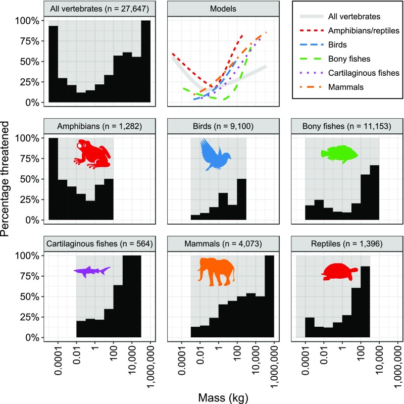
Using a generalized linear mixed-modeling approach, we found that the probability of being threatened was positively and significantly (P < 0.001) related to body mass for birds, cartilaginous fishes, and mammals, but the relationship for all vertebrates pooled was bimodal (P < 0.001) with a breakpoint at 0.035 kg (Fig. 1 and Table S2). By means of segmented-modeling, we also found evidence of bimodal relationships with breakpoints for amphibians/reptiles (0.41 kg) and bony fishes (3.68 kg) (Fig. 1 and Table S2). An order-of-magnitude increase in body mass was associated with estimated increases in the odds of being threatened of 294% for large bony fishes, 184% for large amphibians/reptiles, 107% for birds, 92% for cartilaginous fishes, 67% for mammals, and 27% for large vertebrates pooled, whereas an order-of-magnitude decrease in body mass was associated with increases in the odds of being threatened of 148% for small bony fishes, 153% for small amphibians/reptiles, and 177% for small vertebrates pooled (Fig. 1 and Table S2).

Fig. 1.

Relationships between vertebrate body mass and percentage of species threatened (black histograms) and between mass and probability of being threatened (“Models” graph). Lines in the Models graph indicate the predicted probabilities of being threatened as a function of body mass based on logistic regression models with taxonomic random effects to account for phylogenetic dependence. Segmented models were fitted for all vertebrates, amphibians/reptiles, and bony fishes as these taxa have different (bimodal) body mass–extinction risk relationships at low and high body masses.

Table S2.

Summary of generalized linear mixed models for each taxonomic group

Group	Response	Term	Estimate	Lower	Upper	P value	R2	Estimate*	Lower*	Upper*
All vertebrates	Threatened	Mass (small)	−0.573	−0.666	−0.481	<0.001	0.317†	177%	162%	195%
		Mass (large)	0.237	0.178	0.296	<0.001	0.317†	27%	20%	35%
		Breakpoint	−1.462	−1.542	−1.304		0.317†	0.035	0.029	0.05
		Range size	−1.453	−1.504	−1.403	<0.001	0.66	−77%	−78%	−75%
	Harvesting	Mass	1.115	1.011	1.22	<0.001	0.628	205%	175%	239%
Amphibians	Harvesting	Mass	0.771	0.449	1.094	<0.001	0.155	116%	57%	199%
Amphibians/reptiles	Threatened	Mass (small)	−0.428	−0.554	−0.302	<0.001	0.209†	153%	135%	174%
		Mass (large)	1.043	0.711	1.375	<0.001	0.209†	184%	104%	295%
		Breakpoint	−0.385	−1.058	−0.101		0.209†	0.412	0.087	0.792
		Range size	−1.375	−1.497	−1.253	<0.001	0.716	−75%	−78%	−71%
Birds	Threatened	Mass	0.725	0.58	0.871	<0.001	0.134	107%	79%	139%
		Range size	−1.282	−1.359	−1.205	<0.001	0.587	−72%	−74%	−70%
	Harvesting	Mass	2.242	1.825	2.658	<0.001	0.567	841%	520%	1327%
Bony fishes	Threatened	Mass (small)	−0.395	−0.454	−0.335	<0.001	0.402†	148%	140%	157%
		Mass (large)	1.37	1.106	1.635	<0.001	0.402†	294%	202%	413%
		Breakpoint	0.566	0.134	0.743		0.402†	3.679	1.363	5.532
		Range size	−1.872	−1.991	−1.753	<0.001	0.598	−85%	−86%	−83%
	Harvesting	Mass	0.813	0.697	0.93	<0.001	0.332	126%	101%	153%
Cartilaginous fishes	Threatened	Mass	0.652	0.394	0.909	<0.001	0.311	92%	48%	148%
		Range size	0.114	−0.126	0.354	0.351	0.316	12%	−12%	42%
Mammals	Threatened	mass	0.514	0.406	0.623	<0.001	0.188	67%	50%	87%
		Range size	−1.681	−1.802	−1.56	<0.001	0.724	−81%	−84%	−79%
	Harvesting	Mass	2.416	2.041	2.792	<0.001	0.793	1,021%	670%	1,532%
Reptiles	Harvesting	Mass	0.888	0.523	1.254	<0.001	0.396	143%	69%	250%

Response variables considered were threatened status and whether or not a threatened species is harvested (both binary). No model was fit for cartilaginous fishes and harvesting as insufficient information was available there (all threatened species were harvested). Segmented regression models with respect to body mass were used for species that exhibited different mass-extinction risk relationships at low vs. high masses. For each model, parameter estimates are shown with lower and upper 95% confidence interval endpoints, P values, and pseudo-R². Back-transformed estimates are shown in the columns marked with an asterisk, indicating the change in the odds of being threatened and so forth, associated with a 10-fold increase in mass (or decrease for inverse relationships when using segmented models for modeling threatened status) or range size. The body mass breakpoint estimates and confidence intervals are given in terms of kilograms. Mass and geographic range size were log-transformed for this analysis. Random intercepts were included by taxonomic order (and by class for the “All vertebrates” group) to allow for relationships varying from order to order. Model intercept and random effect estimates are omitted from the table.

^†Pseudo-R² values for the segmented regression models are for the entire model.

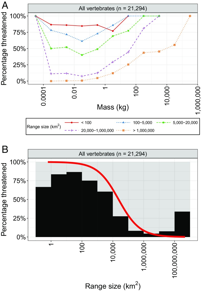
Vertebrates with the largest range sizes were overall less threatened than those with smaller range sizes (Fig. 2 and Figs. S1 and S2). Consistent with this pattern, we found significant (P < 0.001) negative relationships between species range size and the likelihood of species being threatened for all groups except cartilaginous fishes (Fig. S2 and Table S2). Specifically, an order-of-magnitude increase in geographic range size was associated with estimated decreases in the odds of being threatened of 77% for all vertebrates, 75% for amphibians/reptiles, 72% for birds, 85% for bony fish, and 81% for mammals, but an increase of 12% (but not significant, P = 0.351) for cartilaginous fishes (Fig. S2 and Table S2).

Fig. 2.

Effects of range size on the percentage of species threatened. (A) Percentage of species (y axis) within each range size group and mass range (log scale, e.g., 1–10 kg) that are threatened. Only species with IUCN range maps available were used in this plot (totals are shown in panel titles). The relative positions of the lines indicate that range size has a major effect on threatened status regardless of mass. Small range species are generally more threatened than those with large ranges. (B) Relationships between vertebrate geographic range size and percentage of species threatened (black histogram) and between range size and probability of being threatened (red line). The red line indicates the predicted probability of being threatened as a function of range size on a logistic regression model with taxonomic random effects to account for phylogenetic dependence. This result shows that there is a strong negative relationship between range size and probability of being threatened.

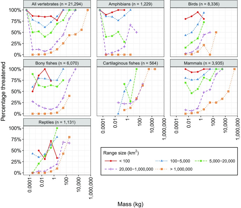
Fig. S1.

For all major classes, percentage of species (y axis) within each range size group and mass range (log scale, e.g., 1–10 kg) that are threatened. Only species with IUCN range maps available were used in this plot (totals are shown in panel titles). The relative positions of the lines indicate that range size has a major effect on threatened status regardless of mass. Small range species are generally more threatened than those with large ranges.

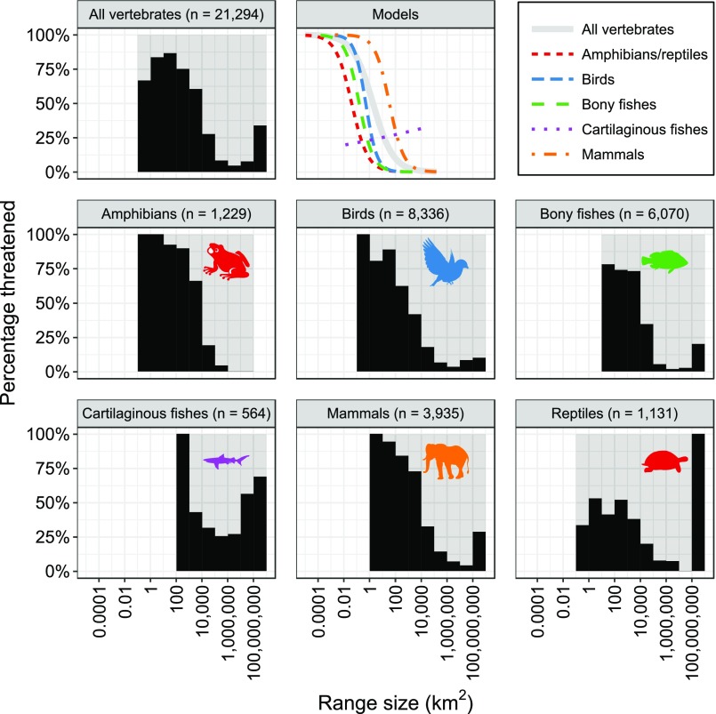
Fig. S2.

For all major classes, relationships between vertebrate geographic range size and probability of being threatened. Lines in the “Models” graph indicate the predicted probabilities of being threatened as a function of range size based on logistic regression models using taxonomic random effects to account for phylogenetic dependence. These results show that there is a strong negative relationship between range size and probability of being threatened for all taxa except cartilaginous fishes.

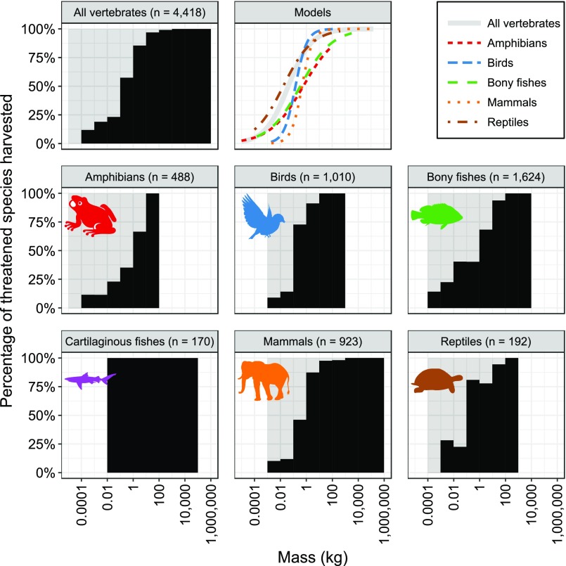
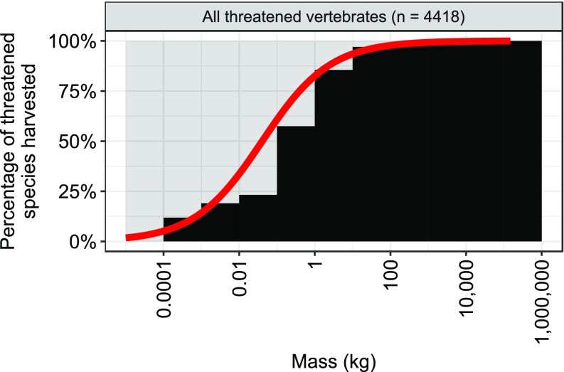
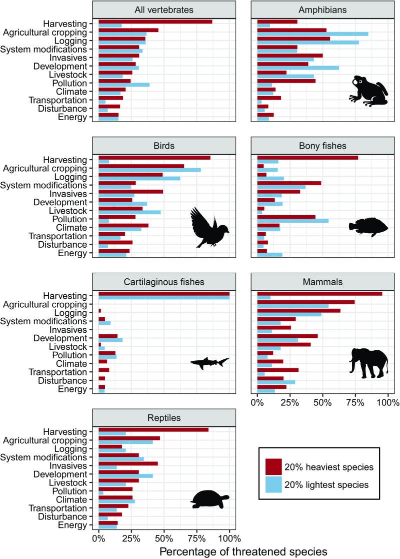
The most common threats faced by all threatened vertebrate species (n = 4,418 with known threat information), in rank order, included harvesting (direct killing by humans), agricultural cropping, logging, and invasive species (Table S3). The probability of being harvested (hunted, trapped, and fished) was significantly and positively related to body mass for threatened species in all vertebrate classes (Fig. S3 and Table S2) (P < 0.001). Moreover, 90% of all threatened vertebrate species larger than 1 kg in body mass were threatened by harvesting (Fig. 3). The strongest effects were found for mammals and birds (Fig. S3), where an order-of-magnitude increase in mass for threatened mammals and birds was associated with an estimated 1,021% and 841% increase, respectively, in the odds of being harvested (Table S2). Harvesting was the most common threat facing the heaviest vertebrates (20% heaviest species in each class) with the exception of amphibians (Fig. 4). Harvesting of the world’s largest vertebrates takes a variety of forms, including regulated and unregulated fishing, trapping, and hunting for meat consumption for subsistence, commercial purposes, or international trade; the use of body parts as medicine, delicacies, or trophies; and killing due to unintentional bycatch (6, 7, 10, 20).

Table S3.

Numbers and proportions of vertebrate species facing each threat type

Threat	Species facing threat	Percent of threatened species, %
Harvesting	1,946	44.05
Agricultural cropping	1,945	44.02
Logging	1,656	37.48
Invasives	1,450	32.82
System modifications	1,370	31.01
Pollution	1,324	29.97
Development	1,188	26.89
Livestock	983	22.25
Climate	921	20.85
Energy	658	14.89
Disturbance	467	10.57
Transportation	459	10.39

The total number of threatened species here is 4,418. Note that this total excludes threatened species that lack threat type information. The numbers of species facing each threat are for threatened species only.

Fig. S3.

Relationships between body mass and probability of being harvested for threatened species in each of the six classes and all vertebrates. Raw data are shown as black histograms. Lines in the “Models” panel indicate the predicted probabilities of threatened species being harvested (killed by humans) as a function of body mass based on logistic regression models using taxonomic random effects to account for phylogenetic dependence. No model was fit for cartilaginous fishes because all threatened species were harvested for this class; however, data for cartilaginous fishes were included in the all vertebrates model. Species totals (n) correspond to number of threatened species only.

Fig. 3.

Relationships between body mass and percentage of threatened species harvested (black histogram) and between mass and probability of being harvested for threatened vertebrates (red line). The red line indicates the predicted probability of threatened species being harvested (killed by humans) as a function of body mass based on a logistic regression model using taxonomic random effects to account for phylogenetic dependence. Species total (n) corresponds to number of threatened species only.

Fig. 4.

Threats to threatened vertebrate species in the top 20% and bottom 20% percentiles for mass within their class. Threats are based on the IUCN Red List threats classification scheme with minor modifications (Methods for details). Within each group, the percentage of threatened species facing each threat is shown for the top 20% heaviest species (red) and 20% lightest (blue) separately. Threats are sorted by the percentage of the heaviest threatened vertebrates (classes pooled) facing each threat. For the all vertebrates grouping (Top Left graph), the lightest 20% of species were all less than 0.0079 kg and the heaviest 20% species were all more than 0.56 kg in body mass.

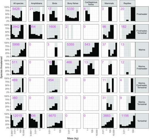
While the heaviest vertebrates are more likely to be threatened by harvesting, the most common threats to the lightest species (20% lightest species in each class) include pollution, agricultural cropping, logging, system modifications, and development (Fig. 4). Most of these species are too small to be intensively harvested for human consumption or other exploitive uses. These threatened light-bodied species are mainly found in freshwater and terrestrial ecosystems, with very few in marine systems (Fig. S4).

Fig. S4.

Histograms showing percentages of species threatened versus body mass. Species are grouped by class (along with all vertebrates together) and types of ecosystem used. Ecosystem type data were obtained from the IUCN Red List. Note that some species may use multiple ecosystem types (e.g., terrestrial and freshwater or marine and freshwater). Numbers of species corresponding to each group and ecosystem type are shown in the panels.

Discussion and Conclusion

Using the most comprehensive dataset on body mass assembled to date, we show how body size can provide a prescriptive estimate of vulnerability to extinction for vertebrates. Our results reveal bimodal relationships between body size and extinction risk for all vertebrates assessed together, amphibians/reptiles, and bony fishes, with small species having an inverse relationship and large species a direct relationship between body mass and extinction risk. Direct relationships between body mass and extinction risk were found for the other vertebrate classes. All relationships were highly significant (P < 0.001) (Table S2).

The principal objective of this study was to investigate patterns of relationships between body size and extinction risk for the world’s vertebrates and to begin to explore possible drivers of this relationship. However, previous research highlights a suite of important predictors of extinction risk, including trophic status, population density, life history, and geographic range size (14, 15, 19, 21, 22). These other drivers have central relevance to the patterns we report as they provide a means for further probing the specific mechanisms that create the observed vulnerabilities to extinction for large and small vertebrates. Range size, in particular, has stood out in other work as a reliable predictor of extinction risk. Specifically, geographic range size was found to be a major predictor for extinction risk in birds (23, 24), some orders of land mammals (15, 19, 21), and squamate reptiles (14). This pattern is supported by our results (Fig. 2B, Fig. S2, and Table S2), which show that range size has a strong negative relationship with extinction risk. Importantly, however, the relationship between body mass and extinction risk does not appear to differ substantially with range size (Fig. 2A and Fig. S1), suggesting that the effects of these two variables are not conflated. More broadly, the acute risks facing small vertebrates apparently are largely because of restricted range-related issues. We note that small range size itself is often not a mechanistic explanation for elevated extinction risk, but is likely related to both intrinsic (life history) and extrinsic (e.g., anthropogenic pressure) drivers of extinction risk (25). Furthermore, it is not surprising that range size is a good predictor of extinction risk because the IUCN Red List process uses restricted range as one of the criteria in determining threatened status (18). Like population size, as range size approaches zero, species approach extinction.

Increasing our understanding of the relationship between body size and extinction risk has practical implications for vertebrate conservation. For example, we too often know little about the biology, spatial ecology, and physiology of many of the world’s most threatened species precisely because of their rarity. For these species, adult body mass is relatively easy to measure and may provide a good first approximation of extinction risk. Our analysis reveals that small and large vertebrates are both at-risk groups, but for a very different set of reasons. Namely, direct killing of animals by harvesting was the dominant threat facing most large vertebrates, whereas the smallest vertebrates were more commonly threatened by habitat loss and modification. Interestingly, the most common threat to all threatened vertebrate species, regardless of body size, was harvesting followed closely by agricultural cropping (Table S3).

The observation that vertebrates at both ends of the size spectrum of life face an increased risk of extinction has important, but quite divergent, consequences for local and global-scale ecological functioning. Large-bodied species, for example, often have larger home ranges and higher overall rates of biomass intake (5). These properties in turn mean that large vertebrates play important roles in controlling how nutrients are vectored across or cycled within ecosystems, how propagules like seeds are distributed, and how well component habitats within ecosystems are interactively connected (4, 26, 27). Larger and often more mechanically powerful species are also frequently identified as ecosystem engineers that shape the physical architecture of ecosystems (28).

Many of the large-bodied vertebrates shown to be at risk in our analysis are predators. These large consumers influence terrestrial, aquatic, and marine food webs from the top down via direct and indirect pathways (9, 29, 30). These species also affect other ecosystem processes, such as biogeochemical cycles, disease, carbon storage, wildfire, and carbon storage (9, 30), and may even buffer communities against climate change (31, 32). By implication, our finding that extinction risk is most acute for large-bodied vertebrates adds to growing concern that loss of top predators will disrupt key species interactions and lead to ecosystem degradation (9).

Losses of small vertebrates come with their own consequences. For example, these species are often important conduits for routing basal energy and biomass into food webs (33), so their loss could compromise ecosystem functioning through diminished bottom-up inputs. Small species also perform unique and important ecological functions that are facilitated by their small body size [e.g., pollination services delivered by bats and hummingbirds (34)]. Accordingly, our findings highlight the danger of focusing disproportionately on the conservation of large-bodied taxa over small-bodied ones. From a human perspective, losses of large and small vertebrates could also be directly consequential. Many cultures, for example, preferentially value and harvest large-bodied vertebrates in both marine and terrestrial ecosystems (27). Likewise, some of the world’s smallest vertebrates, like marine forage fish, are critically important nutrient sources in food systems and can be centerpieces in harvesting economies (35). From an evolutionary perspective, the trends we identify may portend to shifts in the patterns of ecological interactions; changes that could engender important and everlasting evolutionary effects to many components of the ecosystem (36, 37).

Our results describe the relationships between mass and extinction risk and between range size and extinction risk only for species with suitable data available (Table S1). Caution must therefore be used in generalizing to other species for which these data are lacking. However, the species included in our analysis represent a significant portion of the world’s vertebrates. Moreover, there is no clear mechanism by which we would expect species missing from our analysis to have substantially different relationships.

Overall, our finding that at-risk large and small vertebrates face different types of threats suggests that different approaches are needed for the conservation of large versus small species (Fig. 4). For the large species, there is an urgent need to reduce direct killing and consumption of harvest-sensitive species (20). In contrast, for the small-bodied species freshwater and land habitat protection is key because many of these species have highly restricted ranges. Protected areas are likely to directly curb the advance of the kind of place-based threats that it appears smaller vertebrates are facing (38, 39). Indeed, the ranges for many of the smallest threatened vertebrates are concentrated in a few regions and in many cases it would be practical to protect much of these areas (40). For larger vertebrates, such efforts would likely need to be supplemented with programs to responsibly control the harvest of such species in unprotected areas, increase community tolerance of species as they transit between protected zones, and reduce sources of unintentional large vertebrate mortality (41–43). In addition to limiting the proximate threats such as those outlined above, it is important to consider the ultimate threats of human dietary patterns and population growth rates. Increasing rates of human carnivory on the world’s human trophic level (44) is a primary contributor to the overexploitation of the larger vertebrates. Ultimately, reducing global consumption of wild meat is a key step necessary to reduce negative impacts of human hunting, fishing, and trapping on the world’s vertebrates. Furthermore, curtailing the human population growth rate (45) may be the crucial long-term factor in limiting extinction risks to species.

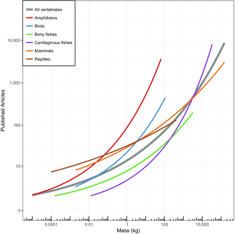
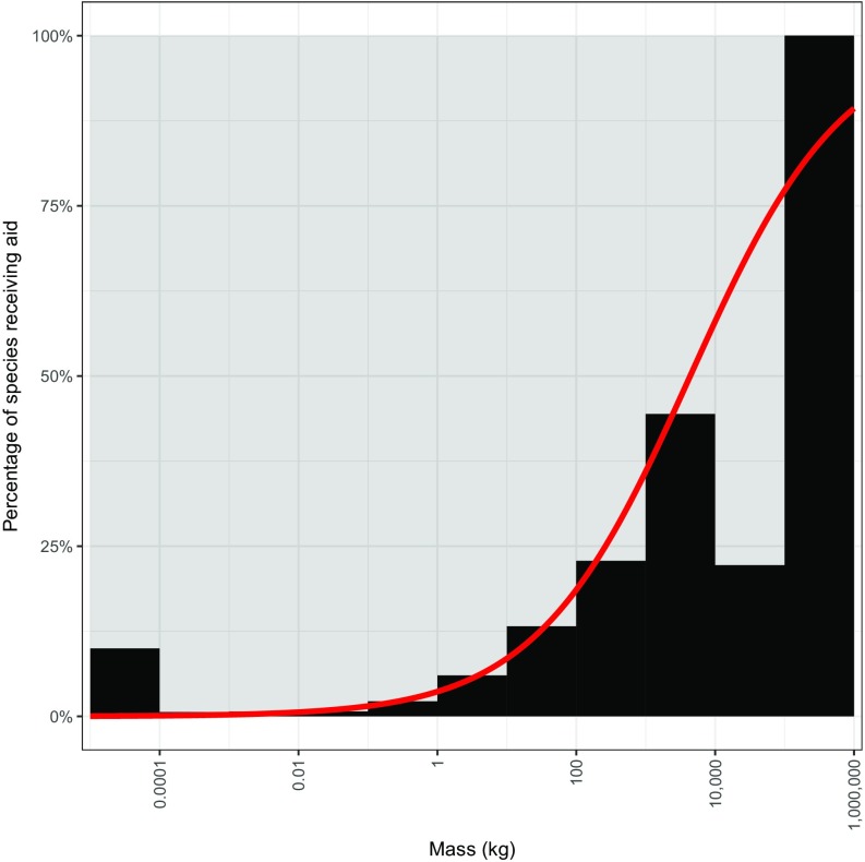
As a group, large animals generally receive more attention and research focus than small ones (Fig. S5), and the vulnerabilities for larger-bodied vertebrates have been drawn out in other more taxonomically focused analyses (10–13). Mammalian megafauna, for example, have been shown to be highly imperiled, with nearly 60% of these species threatened with extinction (1, 7). Likewise, and perhaps accordingly, the larger vertebrates are much more likely to be the target of conservation funding than smaller species (Fig. S6). The overall patterns we report suggest that the vulnerability of smaller vertebrates has been underestimated and underscores the urgent need to increase conservation efforts for both the heaviest and lightest vertebrates. With business as usual, it appears that we will continue to witness a loss of vertebrates from diverse ecosystems around the world (46). Indeed, based on our findings, human activity seems poised to chop off both the head and tail of the size distribution of life. Targeted hunting, fishing, and trapping of large animals is imperiling the largest vertebrates on the planet, whereas habitat modifying activities are endangering, with equal intensity, the smallest vertebrates. This compression of the size distribution of vertebrate life not only represents a radical shift in the living architecture of our planet, but is likely to precipitate consequential shifts in ecological functioning (1, 10, 30).

Fig. S5.

Research effort versus mass for the classes in our analysis. Research effort is measured using number of published articles (1965–2016) for each of the 27,647 species in our analysis. The searches were done in Thomson Reuter’s Web of Science and included taxonomic synonyms as listed on IUCN Red List fact sheets. The lines show negative binomial regression fitted models for each class separately and “all vertebrates” together.

Fig. S6.

Percentages of species receiving financial aid (n = 556 receiving aid). The black histogram (logistic regression fitted model shown in red) indicates a positive association between body mass and the likelihood of receiving aid. Note that the true relationship may differ slightly as some species share common names and some common names may be used in other contexts.

Methods

Mass Database Construction.

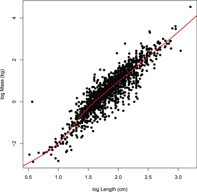
Mammal, bird, and reptile body masses were acquired from the Amniote life-history database (47). To estimate fish masses, we used maximum reported length (by species) data from Fishbase (48). For the 1,735 fish species with known maximum lengths and masses in Fishbase, we modeled the relationship between length and mass (both log-transformed) with a generalized additive model (GAM) fit using the “mgcv” package in R (49, 50). One observation (Micropterus chattahoochae with mass 1 kg and length 3.7 cm) was excluded from the model due to possible inconsistency between mass and length measurements. In addition, the maximum mass for Scomberomorus sinensis was corrected from 131 g to 131 kg. The adjusted R² for the GAM was 0.83 (Fig. S7). We used this model to predict masses for all species in Fishbase with known maximum lengths and unknown masses.

Fig. S7.

Relationship between body mass and maximum length (log scale) for fish using data from FishBase. We used a generalized additive model (fitted relationship shown in red; adjusted R² = 0.825, n = 1734) to predict species body masses from maximum lengths for species with known lengths and unknown masses.

We estimated amphibian masses using data from AmphibiaWeb (51). We did this by first listing all of the species descriptions available on AmphibiaWeb that matched species on the IUCN Red List [excluding species assessed as data deficient (DD), extinct (EX), and extinct in the wild (EW)] and contained a digit followed by “mm” or “cm.” We then looked through these descriptions, recording maximum adult total length (TL) and maximum snout to vent length (SVL) when available. If maximums were not given, we recorded average TL and SVL instead. For the Chinese giant salamander (Andrias davidianus), we used a TL of 158 cm after the largest known living individual (52), rather than the given maximum of 180 cm as the reported maximum was relatively old and may no longer be accurate for this species (51).

We used the lengths obtained from AmphibiaWeb and allometric regression equations (53) to estimate amphibian body masses. For the order Anura, the only equation given was for SVL, so we ran a regression using our amphibian length data to predict SVL from TL (linear model with both variables log-transformed; R² = 0.896) and then used the predicted SVL for species with known TL and unknown SVL. For the other orders, we used either the regression equation based on TL or the equation based on SVL, depending on which amphibian length measurement we had. If both TL and SVL were known, we used both to predict masses separately and then averaged the predictions. We considered the amphibian families Amphiumidae and Sirenidae together to be the legless members of the order Caudata, using the equations for snakes for species in these families.

Geographic Range Size.

We determined range sizes for the species in our analysis using IUCN Red List range maps, when available. For each map, we considered only polygons where a species was classified as “extant” (presence code 1) or “probably extant” (old presence code 2). We then calculated the total area of these polygons for each species using the Mollweide equal-area projection. We grouped species by class and range size (<100 km², 100–5,000 km², 5,000–20,000 km², 20,000–1,000,000 km², >1,000,000 km²) to visualize how mass-extinction risk relationships vary depending on range size. Thresholds for 100 km², 5,000 km², and 20,000 km² correspond to the range thresholds under criterion B of the IUCN Red List categories and criteria.

Extinction Risk.

We joined the data on body masses, rounded to the nearest 0.01 g, obtained from the mass databases (above) with information on species-level extinction risk from the IUCN Red List (v2016.3) (18) using species scientific names and taxonomic synonyms as listed in the IUCN Red List species fact sheets (Table S1). A large number of species with known body masses did not match any species in the IUCN Red List due to not yet being assessed on the IUCN Red List [e.g., while all mammals (54), birds (55), amphibians (56), and sharks (13) have been assessed, reptiles and bony fishes have not yet been completely assessed]. For our analysis, we excluded species listed as DD, EX, or EW, focusing only on those classified as least concern (LC), near threatened (NT), vulnerable (VU), endangered (EN), or critically endangered (CR). Finally, we grouped the species by class: amphibians, mammals, reptiles, birds, bony fishes (Actinopterygii), and cartilaginous fishes (Chondrichthyes). Other fish classes [hagfishes (Myxini), lampreys (Cephalaspidomorphi), and lobe-finned fishes (Sarcopterygii)] were not handled separately, but appear in the results for “all vertebrates.”

Modeling Extinction Risk and Harvesting Threat.

To assess the relationships between body mass and extinction risk and between range size and extinction risk, we treated species as threatened (VU/EN/CR) or nonthreatened (LC/NT) in accordance with the IUCN Red List. We fit generalized linear mixed models separately for each taxonomic class and all vertebrates together. We included random intercepts by taxonomic order (and by class for the “all vertebrates” group) to account for the possibility of mass-extinction risk relationships being more similar within than between orders. Because taxonomically related species tend to be phylogenetically similar, this step helped to account for phylogenetic dependence in the statistical models. Full phylogenetic trees were unavailable for some of the classes in our analysis, precluding the use of more complex modeling techniques like phylogenetic logistic regression (57).

We used a linear model in log mass (i.e., no nonlinear terms) for all groups except amphibians/reptiles, bony fishes, and all vertebrates. For these groups, we used segmented regression models because they exhibited very different mass-extinction risk relationships for small versus large animals. The single breakpoint was estimated by minimizing model deviance and the breakpoint confidence interval was calculated using the profile likelihood. Breakpoint estimation was done using models without taxonomic random effects, but the final segmented models include these random effects. Additionally, we fit separate models for each group of species using only linear terms for range size (log-transformed). We calculated (pseudo) R² including the taxonomic random effects in the variance explained (i.e., conditional R²) using the “sem.model.fits” function in the “PiecewiseSEM” R package (58). A single body mass-based model was fit for amphibians and reptiles together as these classes are similar and there was insufficient data available to fit separate segmented models. Similarly, we combined amphibians and reptiles when using range size as the sole predictor. We repeated this analysis using the binary variable corresponding to whether or not a threatened species is threatened by harvesting as a response. We only used linear models in log mass here as the mass-extinction risk histograms indicated generally monotone relationships.

Extended materials and methods that detail procedures are available in SI Methods, including how we coded IUCN Red List threats, as well as how we quantified research effort and conservation funding.

SI Methods

Coding IUCN Red List Threats.

We used information coded according to the IUCN Red List threats classification scheme to assess threats faced by species. Only threatened species with coded threat information available were used for this portion of the analysis. To separate threats related to livestock and crops, and harvesting and logging, we split two of the top-level threats categories. Specifically, we split the agriculture and aquaculture category 2 into “cropping” (2.1, 2.2) and “livestock” (2.3, 2.4) and the biological resource use category 5 into “harvesting” (5.1, 5.4) and “logging” (5.2, 5.3). Although category 5.2 corresponds to plant gathering (rather than logging), it was uncommon in our dataset as our analysis is restricted to vertebrates. The top-level threats from the threats classification scheme (with subthreats for categories that we split) are listed below with our modifications and titles underlined.

• 1)Residential & commercial development (Development)
• 2)Agriculture & aquaculture (Agricultural cropping for 2.1/2.2, Livestock for 2.3/2.4)
  • 2.1)Annual & perennial nontimber crops
  • 2.2)Wood & pulp plantations
  • 2.3)Livestock farming & ranching
  • 2.4)Marine & freshwater aquaculture
• 3)Energy production & mining (Energy)
• 4)Transportation & service corridors (Transportation)
• 5)Biological resource use (Harvesting for 5.1/5.4, Logging for 5.2/5.3)
  • 5.1)Hunting & collecting terrestrial animals
  • 5.2)Gathering terrestrial plants
  • 5.3)Logging & wood harvesting
  • 5.4)Fishing & harvesting aquatic resources
• 6)Human intrusions & disturbance (Disturbance)
• 7)Natural system modifications (System modifications)
• 8)Invasive & other problematic species, genes & diseases (Invasives)
• 9)Pollution (Pollution)
• 10)Geological events (excluded from our analysis)
• 11)Climate change & severe weather (Climate)
• 12)Other options (excluded from our analysis)

Quantifying Research Effort.

We measured research effort using the number of published articles (1965–2016) for each species in our analysis. The searches were done in Thomson Reuter’s Web of Science and included taxonomic synonyms as listed on species Red List fact sheets. For each species, we searched on topic (title, author, author keywords, Web of Science keywords, and abstract) and recorded the number of results. We modeled the relationship between research effort and (log transformed) body mass using negative binomial regression for all vertebrates together and each class separately.

Quantifying Conservation Funding.

For each species, we searched projects listed in AidData (aiddata.org/) using the species’ common names as listed on its IUCN Red List fact sheet page. Only aid projects with sector “General Environment Protection” and purpose name “Bio-diversity” were considered in the search. Species were classified as receiving aid if one or more of their common names matched the summary text (title, short description, or long description) of at least one project. We then fit a logistic regression model to indicate any association between body mass and the likelihood of vertebrate species receiving financial aid.

Data.

We obtained all of the species body size, status, threat, range, research effort, and conservation funding data used in this project from the public websites described above. The data on these websites are available to all researchers and users should realize that data posted on these websites change over time due to periodical updates.

References

- 1.Ripple WJ, et al. Saving the world’s terrestrial megafauna. Bioscience. 2016;66:807–812. doi: 10.1093/biosci/biw092. [DOI] [PMC free article] [PubMed] [Google Scholar]
- 2.Barnosky AD, et al. Has the Earth’s sixth mass extinction already arrived? Nature. 2011;471:51–57. doi: 10.1038/nature09678. [DOI] [PubMed] [Google Scholar]
- 3.Pimm SL, et al. The biodiversity of species and their rates of extinction, distribution, and protection. Science. 2014;344:1246752. doi: 10.1126/science.1246752. [DOI] [PubMed] [Google Scholar]
- 4.Ceballos G, et al. Accelerated modern human-induced species losses: Entering the sixth mass extinction. Sci Adv. 2015;1:e1400253. doi: 10.1126/sciadv.1400253. [DOI] [PMC free article] [PubMed] [Google Scholar]
- 5.McCauley DJ, et al. Marine defaunation: Animal loss in the global ocean. Science. 2015;347:1255641. doi: 10.1126/science.1255641. [DOI] [PubMed] [Google Scholar]
- 6.Dirzo R, et al. Defaunation in the Anthropocene. Science. 2014;345:401–406. doi: 10.1126/science.1251817. [DOI] [PubMed] [Google Scholar]
- 7.Hoffmann M, et al. The impact of conservation on the status of the world’s vertebrates. Science. 2010;330:1503–1509. doi: 10.1126/science.1194442. [DOI] [PubMed] [Google Scholar]
- 8.Davidson AD, Hamilton MJ, Boyer AG, Brown JH, Ceballos G. Multiple ecological pathways to extinction in mammals. Proc Natl Acad Sci USA. 2009;106:10702–10705. doi: 10.1073/pnas.0901956106. [DOI] [PMC free article] [PubMed] [Google Scholar]
- 9.Estes JA, et al. Trophic downgrading of planet Earth. Science. 2011;333:301–306. doi: 10.1126/science.1205106. [DOI] [PubMed] [Google Scholar]
- 10.Ripple WJ, et al. Collapse of the world’s largest herbivores. Sci Adv. 2015;1:e1400103. doi: 10.1126/sciadv.1400103. [DOI] [PMC free article] [PubMed] [Google Scholar]
- 11.Gaston KJ, Blackburn TM. Birds, body size and the threat of extinction. Philos Trans R Soc Lond B Biol Sci. 1995;347:205–212. [Google Scholar]
- 12.Cardillo M, et al. Multiple causes of high extinction risk in large mammal species. Science. 2005;309:1239–1241. doi: 10.1126/science.1116030. [DOI] [PubMed] [Google Scholar]
- 13.Dulvy NK, et al. Extinction risk and conservation of the world’s sharks and rays. eLife. 2014;3:e00590. doi: 10.7554/eLife.00590. [DOI] [PMC free article] [PubMed] [Google Scholar]
- 14.Böhm M, et al. Correlates of extinction risk in squamate reptiles: The relative importance of biology, geography, threat and range size. Glob Ecol Biogeogr. 2016;25:391–405. [Google Scholar]
- 15.Fritz SA, Bininda-Emonds ORP, Purvis A. Geographical variation in predictors of mammalian extinction risk: Big is bad, but only in the tropics. Ecol Lett. 2009;12:538–549. doi: 10.1111/j.1461-0248.2009.01307.x. [DOI] [PubMed] [Google Scholar]
- 16.Fisher DO, Owens IPF. The comparative method in conservation biology. Trends Ecol Evol. 2004;19:391–398. doi: 10.1016/j.tree.2004.05.004. [DOI] [PubMed] [Google Scholar]
- 17.Olden JD, Hogan ZS, Zanden MJV. Small fish, big fish, red fish, blue fish: Size-biased extinction risk of the world’s freshwater and marine fishes. Glob Ecol Biogeogr. 2007;16:694–701. [Google Scholar]
- 18.IUCN 2017 The IUCN red list of threatened species. Version 2016.3. Available at www.iucnRedList.org. Accessed March 17, 2016.
- 19.Cardillo M, et al. Human population density and extinction risk in the world’s carnivores. PLoS Biol. 2004;2:E197. doi: 10.1371/journal.pbio.0020197. [DOI] [PMC free article] [PubMed] [Google Scholar]
- 20.Ripple WJ, et al. Bushmeat hunting and extinction risk to the world’s mammals. R Soc Open Sci. 2016;3:160498. doi: 10.1098/rsos.160498. [DOI] [PMC free article] [PubMed] [Google Scholar]
- 21.Purvis A, Gittleman JL, Cowlishaw G, Mace GM. Predicting extinction risk in declining species. Proc Biol Sci. 2000;267:1947–1952. doi: 10.1098/rspb.2000.1234. [DOI] [PMC free article] [PubMed] [Google Scholar]
- 22.Owens IPF, Bennett PM. Ecological basis of extinction risk in birds: Habitat loss versus human persecution and introduced predators. Proc Natl Acad Sci USA. 2000;97:12144–12148. doi: 10.1073/pnas.200223397. [DOI] [PMC free article] [PubMed] [Google Scholar]
- 23.Manne LL, Brooks TM, Pimm SL. Relative risk of extinction of passerine birds on continents and islands. Nature. 1999;399:258–261. [Google Scholar]
- 24.Harris G, Pimm SL. Range size and extinction risk in forest birds. Conserv Biol. 2008;22:163–171. doi: 10.1111/j.1523-1739.2007.00798.x. [DOI] [PubMed] [Google Scholar]
- 25.Mace GM, et al. Quantification of extinction risk: IUCN’s system for classifying threatened species. Conserv Biol. 2008;22:1424–1442. doi: 10.1111/j.1523-1739.2008.01044.x. [DOI] [PubMed] [Google Scholar]
- 26.McCauley DJ, et al. Assessing the effects of large mobile predators on ecosystem connectivity. Ecol Appl. 2012;22:1711–1717. doi: 10.1890/11-1653.1. [DOI] [PubMed] [Google Scholar]
- 27.Young HS, McCauley DJ, Galetti M, Dirzo R. Patterns, causes, and consequences of anthropocene defaunation. Annu Rev Ecol Evol Syst. 2016;47:333–358. [Google Scholar]
- 28.Mosepele K, Moyle PB, Merron GS, Purkey DR, Mosepele B. Fish, floods, and ecosystem engineers: Aquatic conservation in the Okavango Delta, Botswana. Bioscience. 2009;59:53–64. [Google Scholar]
- 29.Heithaus MR, Frid A, Wirsing AJ, Worm B. Predicting ecological consequences of marine top predator declines. Trends Ecol Evol. 2008;23:202–210. doi: 10.1016/j.tree.2008.01.003. [DOI] [PubMed] [Google Scholar]
- 30.Ripple WJ, et al. Status and ecological effects of the world’s largest carnivores. Science. 2014;343:1241484. doi: 10.1126/science.1241484. [DOI] [PubMed] [Google Scholar]
- 31.Sala E. Top predators provide insurance against climate change. Trends Ecol Evol. 2006;21:479–480. doi: 10.1016/j.tree.2006.07.006. [DOI] [PubMed] [Google Scholar]
- 32.Wilmers CC, Getz WM. Gray wolves as climate change buffers in Yellowstone. PLoS Biol. 2005;3:e92. doi: 10.1371/journal.pbio.0030092. [DOI] [PMC free article] [PubMed] [Google Scholar]
- 33.Cury PM, et al. Global seabird response to forage fish depletion—One-third for the birds. Science. 2011;334:1703–1706. doi: 10.1126/science.1212928. [DOI] [PubMed] [Google Scholar]
- 34.Stiles GF. Ecological and evolutionary implications of bird pollination. Am Zool. 1978;18:715–727. [Google Scholar]
- 35.Pikitch EK, et al. The global contribution of forage fish to marine fisheries and ecosystems. Fish Fish. 2014;15:43–64. [Google Scholar]
- 36.Galetti M, et al. Functional extinction of birds drives rapid evolutionary changes in seed size. Science. 2013;340:1086–1090. doi: 10.1126/science.1233774. [DOI] [PubMed] [Google Scholar]
- 37.Galetti M, Dirzo R. Ecological and evolutionary consequences of living in a defaunated world. Biol Conserv. 2013;163:1–6. [Google Scholar]
- 38.Lester S, et al. Biological effects within no-take marine reserves: A global synthesis. Mar Ecol Prog Ser. 2009;384:33–46. [Google Scholar]
- 39.Geldmann J, et al. Effectiveness of terrestrial protected areas in reducing habitat loss and population declines. Biol Conserv. 2013;161:230–238. [Google Scholar]
- 40.Myers N, Mittermeier RA, Mittermeier CG, da Fonseca GA, Kent J. Biodiversity hotspots for conservation priorities. Nature. 2000;403:853–858. doi: 10.1038/35002501. [DOI] [PubMed] [Google Scholar]
- 41.Dickman AJ. Complexities of conflict: The importance of considering social factors for effectively resolving human-wildlife conflict. Anim Conserv. 2010;13:458–466. [Google Scholar]
- 42.Vanderlaan ASM, Taggart CT. Vessel collisions with whales: The probability of lethal injury based on vessel speed. Mar Mamm Sci. 2007;23:144–156. [Google Scholar]
- 43.Hilborn R. Policy: Marine biodiversity needs more than protection. Nature. 2016;535:224–226. doi: 10.1038/535224a. [DOI] [PubMed] [Google Scholar]
- 44.Bonhommeau S, et al. Eating up the world’s food web and the human trophic level. Proc Natl Acad Sci USA. 2013;110:20617–20620. doi: 10.1073/pnas.1305827110. [DOI] [PMC free article] [PubMed] [Google Scholar]
- 45.Gerland P, et al. World population stabilization unlikely this century. Science. 2014;346:234–237. doi: 10.1126/science.1257469. [DOI] [PMC free article] [PubMed] [Google Scholar]
- 46.Visconti P, et al. Projecting global biodiversity indicators under future development scenarios: Projecting biodiversity indicators. Conserv Lett. 2016;9:5–13. [Google Scholar]
- 47.Myhrvold NP, et al. An amniote life-history database to perform comparative analyses with birds, mammals, and reptiles. Ecology. 2015;96:3109. [Google Scholar]
- 48.Froese R, Pauly D. 2000 FishBase. Available at www.fishbase.org/home.htm. Accessed September 16, 2016.
- 49.Wood SN. mgcv: GAMs and generalized ridge regression for R. R News. 2001;1:20–25. [Google Scholar]
- 50.R Development Core Team 2009. R: A Language and Environment for Statistical Computing (R Foundation for Statistical Computing, Vienna, Austria),Version 2.92.
- 51.AmphibiaWeb 2016 Berkeley, California: AmphibiaWeb: Information on amphibian biology and conservation. Available at amphibiaweb.org/. Accessed August 19, 2016.
- 52.Prague Zoo 2015 Prague Zoo displays probably the largest Giant Salamander in the world. Available at https://www.zoopraha.cz/en/about-zoo/news/9600-prague-zoo-displays-probably-the-largest-giant-salamander-in-the-world. Accessed September 16, 2016.
- 53.Pough FH. The advantages of ectothermy for tetrapods. Am Nat. 1980;115:92–112. [Google Scholar]
- 54.Schipper J, et al. The status of the world’s land and marine mammals: diversity, threat, and knowledge. Science. 2008;322:225–230. doi: 10.1126/science.1165115. [DOI] [PubMed] [Google Scholar]
- 55.BirdLife International 2016 IUCN Red List for birds. Available at www.birdlife.org. Accessed November 18, 2016.
- 56.Stuart SN, et al. Status and trends of amphibian declines and extinctions worldwide. Science. 2004;306:1783–1786. doi: 10.1126/science.1103538. [DOI] [PubMed] [Google Scholar]
- 57.Ives AR, Garland T., Jr Phylogenetic logistic regression for binary dependent variables. Syst Biol. 2010;59:9–26. doi: 10.1093/sysbio/syp074. [DOI] [PubMed] [Google Scholar]
- 58.Lefcheck JS. piecewiseSEM: Piecewise structural equation modeling in R for ecology, evolution, and systematics. Methods Ecol Evol. 2016;7:573–579. [Google Scholar]