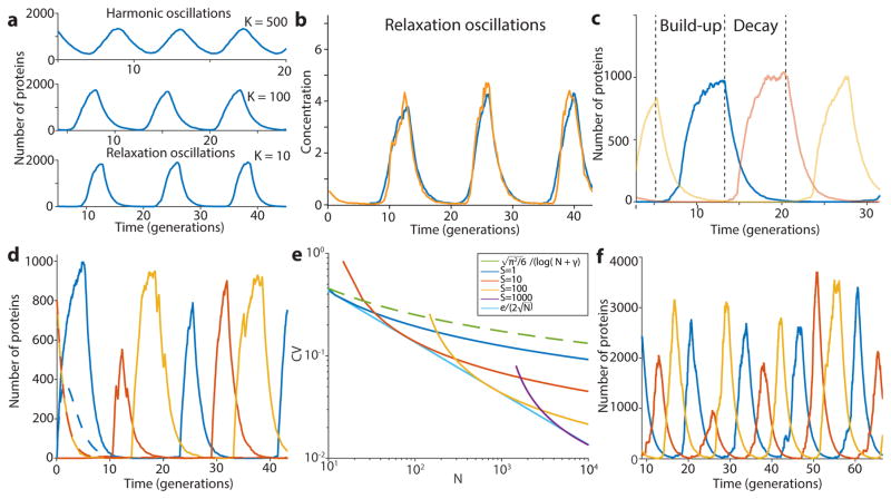
Extended Data Figure 4.

Modeling results. a) The repressilator can display harmonic or relaxation oscillations. The gradual transition between the regimes is shown here by varying the parameter K in the minimal model (λ = 2000 and n = 4, SI §4.1). b) The experimental data suggest that the repressilator oscillates in the relaxation regime. Simulated time trace (blue, K = 13, λ = 10³, and n = 3 ) is overlayed with time trace of experimental data (from Fig. 2c, LPT64, yellow). c) Close-up of a simulated time trace (minimal model, K = 0.2, λ = 10³, and n = 2, SI §4.1) in the relaxation regime showing the three different repressors (blue, red and yellow). The oscillations can be separated in two distinct phases: an accumulation phase during which the protein (blue) is completely derepressed (red below threshold) and starts at very low numbers, and a decay phase that starts when the repressor is completely repressed (red above threshold) and ends when it goes below the repression threshold of the next component (yellow starts to accumulate). d) Relaxation oscillators have different parameter requirements for oscillations. Simulated time traces (solid lines) show oscillations without biochemical cooperativity or phase shift due to the presence of mRNA (minimal model, K = 0.01, λ = 10³, and n = 1, SI §4.1). The deterministic differential equations with the same parameters show damped oscillations (dashed lines with flipped colors). e) Even for perfect threshold mechanism, significant noise comes from the decay phase if the threshold (S) is too low (or too high) with respect to the peak value (N). If S ≪ N, then the CV in one decay step goes down very slowly (1/log(N/(S + 1))). However, if it is reasonably close to its optimal value (e.g. 0.05 < S/N < 0.3), it goes down much faster ( $1/\sqrt{N}$). The CV is shown for different combination of S and N, as well as the asymptotic traces. f) Simulated time trace of the model of SI §4.3.1 shows oscillations of similar shape, peak amplitude numbers, period and phase drift as the experimental data by using reasonable parameters (λ = 60, K = (5, 10, 10) for the three repressors, n = 1.5 for all repressors, 〈b〉 = 10, 〈N_o〉 = 10 〈N_t〉 = 40).