LCN: a random graph mixture model for community detection in functional brain networks

Abstract

The aim of this article is to develop a Bayesian random graph mixture model (RGMM) to detect the latent class network (LCN) structure of brain connectivity networks and estimate the parameters governing this structure. The use of conjugate priors for unknown parameters leads to efficient estimation, and a well-known nonidentifiability issue is avoided by a particular parameterization of the stochastic block model (SBM). Posterior computation proceeds via an efficient Markov Chain Monte Carlo algorithm. Simulations demonstrate that LCN outperforms several other competing methods for community detection in weighted networks, and we apply our RGMM to estimate the latent community structures in the functional resting brain networks of 185 subjects from the ADHD-200 sample. We find overlap in the estimated community structure across subjects, but also heterogeneity even within a given diagnosis group.

1. Introduction

A problem of particular interest in the field of neuroscience is to understand the structure and organization of functional and structural brain networks and their relationships with predictors such as disease status and behavior [16, 3]. The existing literature has largely focused on various topological measures, such as degree distribution, clustering coefficient and network diameter, and their clinical implications [3, 26, 14, 9]. These types of global and local network characteristics are convenient in their ability to reduce large networks to a small set of statistics that describe their large-scale organization. The community network structure, in which there exist groups of nodes (sometimes called “modules”) that have dense connections within each group and sparse connections between different groups, has been observed in numerous real life networks [34, 10, 7, 15, 33], including functional brain networks [26, 16]. See [7] for a comprehensive review of various approaches to the community detection problem.

Our motivating data are resting-state functional magnetic resonance images (fMRI) from the ADHD-200 sample, which is downloadable from http://fcon_1000.projects.nitrc.org/indi/adhd200. In this study, we have used the dataset with 215 subjects collected at New York University. After removing the ADHD hyperactive/impulsive subtype due to a small sample size, our analysis dataset consists of 185 subjects: 91 typically developing controls, 62 of the ADHD combined subtype, and 32 of the ADHD inattentive subtype. For each subject, we calculated a 116 × 116 Fisher-transformed correlation matrix based on the 116 predefined regions of interest (ROI) defined by the automated anatomical labeling (AAL) template [30] and used it as a resting-state fMRI connectivity network. See Figure 1 for the networks of two randomly selected subjects, which have been visualized with the BrainNet Viewer (http://www.nitrc.org/projects/bnv/) [32]. Thus, our networks consist of 116 nodes (brain regions) and the weighted edges between them (Fisher-transformed correlations between time courses). We are interested in understanding the modular structure of these functional brain networks, which we address by formulating a Bayesian random graph mixture model to detect the latent community structure in each network and estimate the modularity parameters governing the edge weights.

Figure 1.

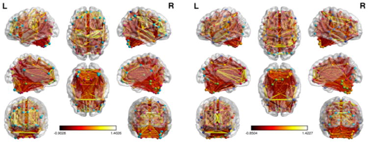
Functional brain networks for subject 1 (L) and subject 2 (R). There are 116 brain regions in each image. Different colored nodes indicate different estimated latent classes, but colors are not comparable between subjects.

Two major classes of community detection methods include optimization algorithms and model-based methods. The typical approach to model-based community detection is via the stochastic block model (SBM), which summarizes the network characteristics through a low dimensional latent space, while partitioning the network into blocks of nodes with similar connectivity characteristics [20, 17, 18]. The SBM can be seen as an extension of the well-known Erdős-Rényi random graph model for binary graphs [6]. While much of the focus has been on binary graphs (e.g. Nowicki and Snijders [20], Choi, Wolfe and Airoldi [4], Vu, Hunter and Schweinberger [31], Schweinberger and Handcock [24]), versions of the SBM have been proposed to estimate the community structure of random weighted graphs [17]. However, calculating unknown parameters in these SBMs represents major computational challenges. For instance, maximum likelihood estimation is only possible for small graphs due to the intractable summation in the EM algorithm for the SBM likelihood [27]. Alternatively, Bayesian methods based on Markov chain Monte Carlo (MCMC) sampling and variational algorithms have been developed for the calculation of posterior estimates for the SBM [17, 12, 1]. Moreover, other approximating methods, such as the use of a composite likelihood and moment estimators, have been proposed to compute parameter estimates for some versions of the SBM [2].

In this paper, we develop a fully Bayesian framework for the weighted SBM as a hierarchical random graph mixture model (RGMM), in order to estimate the latent class network (LCN) structure in functional brain networks. We propose conjugate priors for the unknown parameters in order to achieve efficient estimation and use the more parsimonious affiliation version of the SBM to avoid a well-known nonidentifiability issue. We develop an efficient Markov chain Monte Carlo (MCMC) algorithm to draw random samples from the desired posterior distribution. Our MCMC algorithm can handle graphs with thousands of nodes or relatively few nodes without having to rely on any asymptotic assumptions or approximations. Our simulations demonstrate that our estimation approach outperforms several existing methods for the weighted SBM in terms of both classification accuracy and accuracy in estimating the modularity parameters, and we apply our method to the sample of functional brain networks and examine the patterns of estimated latent community structure across children from different ADHD diagnosis groups.

The rest of the article is organized as follows. Section 2 introduces the formulation of our random graph mixture model and its associated MCMC sampling algorithm. In Section 3, we compare our method to several competing methods using simulated data. Then in Section 4, we apply our method to the functional brain network dataset discussed above. In Section 5, we present some concluding remarks.

2. Methodology

2.1 Random graph mixture model

Let Y = (Y_ij) denote an observed undirected graph with n nodes, where Y_ij denotes the weighted edge value between node i and node j. We assume that the n nodes each fall into one of Q latent classes, with the unobserved class label of node i given by the random vector Z_i = (Z_i1,… Z_iQ), where Z_iq = 1 indicates that node i is in the q–th group. Following the version of the SBM in [2], our RGMM consists of:

1. A latent class model for characterizing the class label Z_i for each node i = 1,… n.

2. A measurement model for characterizing the conditional distribution of Y_ij given {Z_i, Z_j}.

We assume that the latent classes {Z_i} are independently and identically distributed as Multinomial random variables with the probability vector π = (π₁, … π_Q) such that 0 ≤ π_q ≤ 1 and Σ_q π_q = 1. The measurement model is a two-component mixture model: we assume that Y_ij conditional on {Z_i}_1≤i≤n are independent and the conditional distribution of Y_ij given Z_ic · Z_jd = 1 is given by

$$p_{cd}f(\cdot ;{\theta }_{cd})+(1-p_{cd}){\delta }_0(\cdot )\text{for}i,j=1,\dots n,$$

where f(·; θ_cd) is a prefixed probability distribution with an unknown parameter vector θ_cd and δ₀(·) denotes the Dirac measure at zero accounting for non-present edges. By assuming that the edge values are conditionally independent given the latent classes of the nodes, the (marginal) dependencies of the graph are fully determined by the latent community structure.

Furthermore, we impose the affiliation SBM by reducing the Q · (Q + 1) parameters in {p_cd}_{1≤c≤d≤Q} and {θ_cd}_{1≤c≤d≤Q} to:

$$p_{cd}=\{\begin{array}{cc}{p}_{\mathit{\text{in}}}& \text{if}c=d,\\ p_{\mathit{\text{out}}}& \text{if}c\ne d,\end{array}\text{and}{\theta }_{cd}=\{\begin{array}{cc}{\theta }_{\mathit{\text{in}}}& \text{if}c=d,\\ {\theta }_{\mathit{\text{out}}}& \text{if}c\ne d.\end{array}$$

Use of this parameterization allows us to avoid the typical problem of label switching/swapping in Bayesian mixture modeling. When non-symmetric priors are used for the group proportions, the nonidentifiability of the order of the latent classes of nodes can lead to the class labels changing between successive MCMC samples and make posterior inference difficult. The affiliation SBM does not have class-specific parameters, so the sampler arbitrarily sets the order in the initialization step and then sampling proceeds without label swapping.

This framework is flexible and can model directed graphs by utilizing a bivariate distribution for f(Y_ij, Y_ji) and allowing p_cd ≠ p_dc and θ_cd ≠ θ_dc. Here we focus on Gaussian-weighted edges, such that θ = (θ_in, θ_out) = (μ_in, τ_in, μ_out, τ_out), but we can easily incorporate different distributions for the edge distribution f(·). We can also adapt the model for more complex latent structures such as the overlapping SBM and correlated latent groups by alterations within this hierarchical formulation.

2.2 Prior distributions

Priors are chosen to preserve conjugacy to allow for efficient MCMC estimation as follows:

$$\begin{array}{cc}\pi |Q~\text{Dirichlet}(a_1,\dots a_Q),& P_{\mathit{\text{in}}},P_{\mathit{\text{out}}}~\text{Uniform}(0,1),\\ {\mu }_{\mathit{\text{in}}}|{\tau }_{\mathit{\text{in}}}~N({\mu }_{0,\mathit{\text{in}}},\frac{{\sigma }_{0,\mathit{\text{in}}}^2}{{\tau }_{\mathit{\text{in}}}}),& {\mu }_{\mathit{\text{out}}}|{\tau }_{\mathit{\text{out}}}~N({\mu }_{0,\mathit{\text{out}}},\frac{{\sigma }_{0,\mathit{\text{out}}}^2}{{\tau }_{\mathit{\text{out}}}}),\\ {\tau }_{\mathit{\text{in}}}~\text{Ga}({\alpha }_{0,\mathit{\text{in}}},{\beta }_{0,\mathit{\text{in}}}),& {\tau }_{\mathit{\text{out}}}~\text{Ga}({\alpha }_{0,\mathit{\text{out}}},{\beta }_{0,\mathit{\text{out}}}),\end{array}$$

where Ga(a, b) is a gamma distribution with shape a and rate b. To achieve relatively flat priors, we set the hyperparameters to be: a₁,… a_Q = 1, μ_0,in = μ_0,out = 0, ${\sigma }_{0,\mathit{\text{in}}}^2={\sigma }_{0,\mathit{\text{out}}}^2=10$, and α_0,in = α_0,out = β_0,in = β_0,out =0.01.

2.3 Estimation

We utilize a Gibbs sampler for posterior computation, with all full conditional posterior distributions given in the Appendix. The Gibbs sampler involves sampling from a series of conditional distributions while each of the components is updated in turn. Our Gibbs sampler starts as follows:

• Initialize ${\pi }_q^{(0)}=1/Q$ for q = 1,… Q.

• Sample $Z_i^{(0)}$ from Dirichlet(π⁽⁰)) for i = 1,… n.

• Initialize $p_{\mathit{\text{in}}}^{(0)}=p_{\mathit{\text{out}}}^{(0)}=\frac{1}{2}$, ${\mu }_{\mathit{\text{in}}}^{(0)}={\mu }_{\mathit{\text{out}}}^{(0)}=0$, ${\tau }_{\mathit{\text{in}}}^{(0)}={\tau }_{\mathit{\text{out}}}^{(0)}=1$.

Then for t = 1,… N, we sequentially update all parameters as follows:

• Sample π^(t) from P(π|Q, Y, Z^(t−1)).

• For i = 1,… n, sample $Z_i^{(t)}$ from

  $$P(Z_i|Q,Y,Z_{1:(i-1)}^{(t)},Z_{(i+1):n}^{(t-1)},{\pi }^{(t)},P_{\mathit{\text{in}}}^{(t-1)},P_{\mathit{\text{out}}}^{(t-1)},{\mu }_{\mathit{\text{in}}}^{(t-1)},{\mu }_{\mathit{\text{out}}}^{(t-1)},{\tau }_{\mathit{\text{in}}}^{(t-1)},{\tau }_{\mathit{\text{out}}}^{(t-1)}).$$

• Sample ${\mu }_{\mathit{\text{in}}}^{(t)}$ from $P({\mu }_{\mathit{\text{in}}}|Q,Y,Z^{(t)},{\tau }_{\mathit{\text{in}}}^{(t-1)})$ and ${\mu }_{\mathit{\text{out}}}^{(t)}$ from $P({\mu }_{\mathit{\text{out}}}|Q,Y,Z^{(t)},{\tau }_{\mathit{\text{out}}}^{(t-1)})$.

• Sample ${\tau }_{\mathit{\text{in}}}^{(t)}$ from $P({\tau }_{\mathit{\text{in}}}|Y,Z^{(t)},{\mu }_{\mathit{\text{in}}}^{(t)})$ and ${\tau }_{\mathit{\text{out}}}^{(t)}$ from $P({\tau }_{\mathit{\text{out}}}|Y,Z^{(t)},{\mu }_{\mathit{\text{out}}}^{(t)})$.

• Sample $p_{\mathit{\text{in}}}^{(t)}$ from P(p_in|Y, Z^(t)) and $p_{\mathit{\text{out}}}^{(t)}$ from P(p_out|Y, Z^(t)).

To improve sampling performance, we run multiple MCMC chains and use the Integrated Completed Likelihood (ICL) criterion to automatically select the chain that maximizes ICL [17, 5]. For a graph with n nodes, the ICL criterion is given by:

$${\text{ICL}}_Q=\underset{\theta }{max}log\mathbb{P}(Y,\stackrel{\sim }{Z}|Q,\theta )-\frac{1}{2}[P_Q\cdot log\left(\frac{n(n-1)}{2}\right)+(Q-1)\cdot log(n)],$$ (1)

where Ẑ denotes the predictions for the latent Z and P_Q denotes the number of independent parameters. In this case, we have θ = (p_in, p_out, μ_in, μ_out, τ_in, τ_out) and P_Q = 6. Moreover, we plug in the univariate mode of each parameter into ICL_Q. This amounts to maximizing the observed data likelihood when comparing two MCMC chains with Q and n fixed.

To achieve better sampling performance for large graphs, we propose using spectral clustering to estimate the initial value of the latent structure Z⁽⁰⁾; we can use the k-means clustering algorithm [11] to cluster all n nodes into Q groups according to the first Q eigenvectors of a graph. Moreover, the diagnostic tools in the coda R package [22] can be used to assess posterior convergence.

3. Simulations

We carried out simulations to examine the finite sample performance of the LCN RGMM in detecting the community structure of simulated networks and quantify their network modularity.

3.1 Setup

We simulated networks as follows: for a given Q_*, π was randomly generated from Dirichlet(a₁,… a_Q*), and then each Z_i for i = 1,… n was independently generated from Multinomial(π₁,… π_Q*). The data Y_ij were generated from a mixture of zero-valued edges, randomly drawn from either Bernoulli(1−p_in) or Bernoulli(1−p_out) distributions and either Normal(μ_in, ${\tau }_{\mathit{\text{in}}}^{-1}$) or Normal(μ_out, ${\tau }_{\mathit{\text{out}}}^{-1}$), depending on whether nodes i and j are in the same latent class. We set hyper-parameters ${\sigma }_{0,\mathit{\text{in}}}^2$ and ${\sigma }_{0,\mathit{\text{out}}}^2$ to one. The parameters p_in, p_out, μ_in, μ_out, τ_in, and τ_out, were fixed at various values in order to examine the finite sample performance of LCN and the associated MCMC algorithm as modularity measures change.

We considered six schemes and simulated 200 independent graphs for each scheme. Simulation schemes are listed in Table 1. Scheme 1 is an example of a relatively easy community detection problem with p_in ≫ p_out and μ_in ≫ μ_out. Scheme 2 is a much harder problem with decreased distance between mixture distributions and fully dense graphs (no zero edges). Schemes 3 and 5 were designed to test performance when the number of latent groups is misspecified. Scheme 4 represents a scenario with a large number of nodes. Scheme 6 is a scenario with a relatively large number of smaller latent groups.

Table 1. 200 datasets were simulated from each of these schemes, then analyzed using 2 MCMC chains, and the chain with the greatest ICL was selected.

Sim	n	Q*	Q (est)	pin	pout	μin	μout	τin	τout
1	50	3	3	0.8	0.3	1	-1	1	1
2	50	3	3	1	1	0.5	-0.3	0.2	0.4
3	50	3	5	0.8	0.3	1	-1	1	1
4	500	3	3	0.8	0.3	0.5	-0.5	1	1
5	100	5	10	0.8	0.3	0.5	-0.5	1	1
6	50	10	10	0.8	0.3	0.5	-0.5	1	1

For each graph, we ran two independent chains of the Gibbs sampler and then used ICL to choose the best chain as described previously. We also compared our method with several methods for community detection in weighted graphs: the approximating method of Ambroise and Matias based on a composite likelihood [2] (AM), the Bayesian implementation of the original SBM of Nowicki and Snijders in the hergm R package [20, 28, 25] (HERGM), the spin-glass model of [23] (SPIN) [19, 29], and a simple spectral clustering algorithm, using k-means [11] on the eigenvectors of the adjacency matrix (SPEC). To deal with the label switching phenomenon seen in the hergm output, MCMC samples were relabeled with the use of the loss function from Carvalho (2013) [21], which is included in the R function hergm.postprocess.

3.2 Results

Classification is typically accurate under all of the simulation schemes, as shown via box plots of the misclassification rates in Figure 2, though expectedly less so with more similar mixture distributions. The most probable classes were estimated from the 10,000 MCMC samples for each simulation, and the misclassification rate was estimated as the sum of false positives (nodes estimated to be in the same community when they are not) and false negatives (nodes estimated to be in different communities when they are in the same) divided by the total number of possible latent connections (n · (n − 1)/2). Most misclassification occurred in MCMC chains that did not converge to the true posterior distribution, which is seen in the tails of the box plots – many of these incorrectly estimated a single latent class containing all the nodes.

Figure 2.

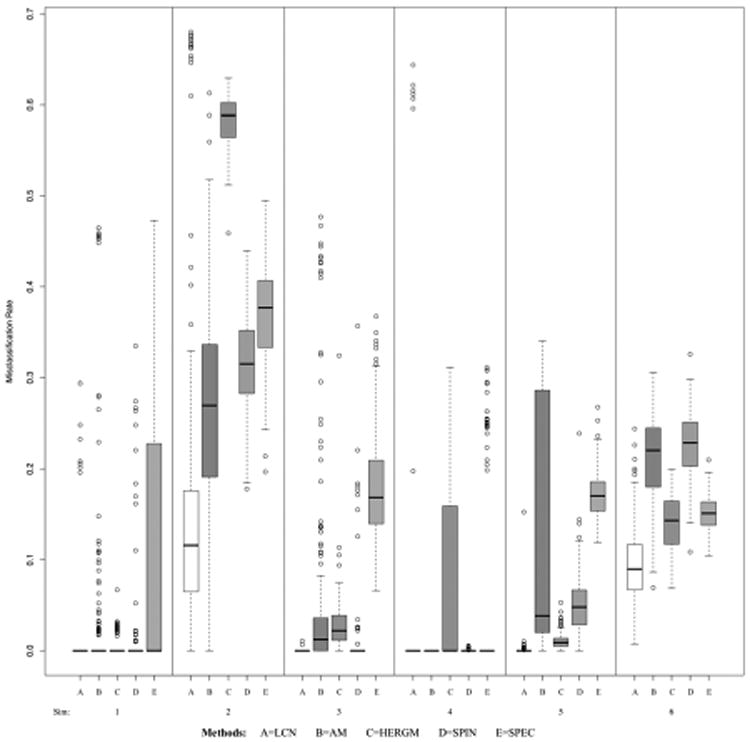
Boxplots of misclassification rates by simulation scheme. The 6 schemes, each with 200 simulated datasets, are listed in Table 1. Misclassification rate is defined as the sum of the false positives and false negatives divided by the total number of possible node pairs.

The methods mostly do well for the “easy” community detection problem (Scheme 1). Our method outperformed the other methods for the selection of the true number of groups when more groups were specified (Schemes 3 and 5). The approximating method of Ambroise and Matias (AM) fares well with a large number of nodes (Scheme 4), but it is not as accurate for smaller graphs (Schemes 2 and 6). The Bayesian method (HERGM) [20, 28, 25] is approximately exact, but it involves a computationally intensive algorithm for solving the label switching problem, which adds another level of error in estimating the latent structure, especially in the difficult Scheme 2. The spin-glass method (SPIN) [19, 29], which is based on extension of modularity maximization to networks with positive and negative weights, tends to be accurate in classification but less so in Scheme 6, where there are a greater number of smaller groups; it has been shown previously that modularity optimization methods can fail to detect communities that are smaller than a value which depends on the total network size and the connectedness of separate communities [8]. The simple spectral clustering algorithm (SPEC) only performs well in Scheme 4, where the simulated networks are larger than in the other schemes.

In our estimation method, when the MCMC chain converges to the true distribution, estimation of the other parameters is accurate. Figure 3 shows the absolute deviation from between the posterior median and the true parameter value, scaled by the magnitude of the parameter. For the edge parameters (μ_in, μ_out, τ_in, τ_out) estimated in both our formulation and the parameterization used in [2], our approach typically has less estimation error. Figure 4 gives coverage of the 95% highest posterior density (HPD) regions for the edge parameters; coverage is near 95% for most edge parameters, except for p_in and p_out in Scheme 2 − in which the parameters are on the boundary of the parameter space. For large graphs such as in Scheme 4, decreasing HPD widths indicate efficient estimation of the edge parameters.

Figure 3.

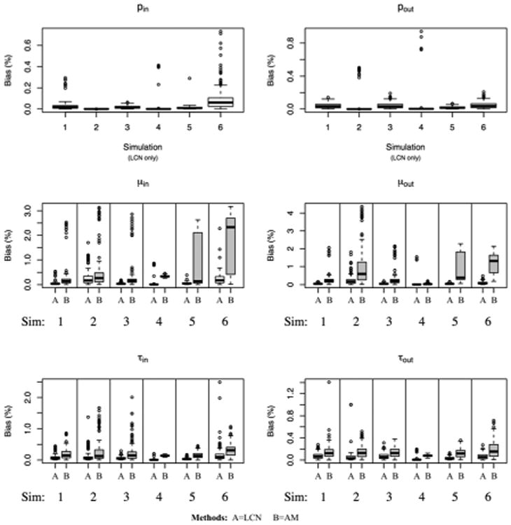
Absolute deviation between the posterior median of each parameter and the true value, scaled by the true value, from each of the 6 schemes listed in Table 1. For the edge parameters μ_in, μ_out, τ_in, τ_out, results from our Bayesian random graph model (A – on the left of each panel) are compared to the method of Ambroise and Matias (B – on right).

Figure 4.

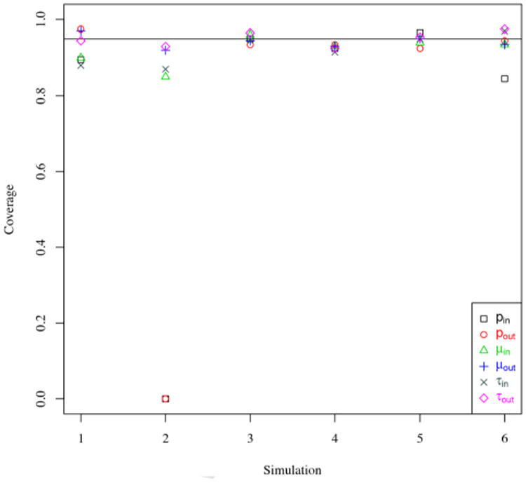
Percent of the 95% HPD intervals containing the true value, across 200 simulations in each scheme. Simulation schemes are listed in Table 1. The horizontal line indicates 95%.

4. ADHD-200 Resting-State FMRI Networks

The resting state fMRI scans were acquired using a Siemens Allegra 3T scanner for six minutes (voxel size = 3 × 3 × 4mm, slice thickness = 4mm, number of slices=33, TR=2s, TE=15ms, flip angle=90°, field of view=240mm). The Athena pipeline was applied for data preprocessing and the images were band-pass filtered within a frequency range of (0.009, 0.08) hz. We deleted the scans showing movement artifacts or other problems based on the quality control information given in the phenotypic dataset and then, for the subjects with at least one scan passing quality control, we selected a single scan for calculation of that subject's connectivity network.

The automated anatomical labeling (AAL) template [30] was used to split patients' brains into 116 non-overlapping regions of interest (ROIs); blood-oxygen-level dependent (BOLD) contrast signals were averaged within each region for each of 172 time points, and a Pearson correlation matrix was estimated for each subject's 116 ROI × 172 time point matrix. Subsequently, the elements in each 116 × 116 matrix were transformed to approximate normality via the Fisher transformation, $z=0.5\times ln\left(\frac{1+r}{1-r}\right)$. Additionally, the Fisher-transformed correlation matrices were thresholded at ± 0.1 (which corresponds to r ∼ ±0.1) to allow for some level of sparsity.

We applied our RGMM to each subject's weighted network as follows: two parallel MCMC chains of our Gibbs sampling algorithm were run for each of Q = 3, 6, 9, and 12, and then ICL was used to choose the best of the 8 chains, which allowed for anywhere between 1 and 12 latent classes for each subject. Figure 1 shows the estimated latent classes of the 116 ROIs for two randomly selected subjects as the color of nodes in the networks; subject 1 (L) has 7 latent classes of regions and subject 2 (R) has 8 latent classes of regions. To assess the overlap of the community structures of the two subjects, the adjusted Rand Index [13] between the two clusterings was estimated to be 0.182, which is significantly different from zero (which would indicate no overlap at all) via permutation testing (10,000 permutations of the class labels, p < 0.001). So, while the latent community structure for these two subjects is different, there is significant overlap between them, which suggests that there may be a shared latent structure and individual deviations from this structure.

Figure 6 shows the estimated number of latent classes across the 185 subjects, with values ranging from 2 to 9; more than half of the subjects have either 4 or 5 estimated latent classes of ROIs. In Figure 7, the overlap of the latent structures of all 185 subjects is shown; the node pairs in red are those that are in the same latent class in most networks, while the node pairs in green are in different latent classes in most networks. The functional overlap between these node pairs could be considered as the shared latent functional brain structure, while other groups of node pairs are in the same latent classes in only a subset of the subjects (see the node pairs in black, which have been estimated to be in the same latent class in approximately 50% of subjects). Additionally, the posterior distributions of the modularity parameters appear to vary across many of the subjects, indicating heterogeneity in latent community structure even beyond the latent class membership of the 116 ROIs. See Figure 5 for posterior samples of the modularity parameters of the two subjects from Figure 1.

Figure 6.

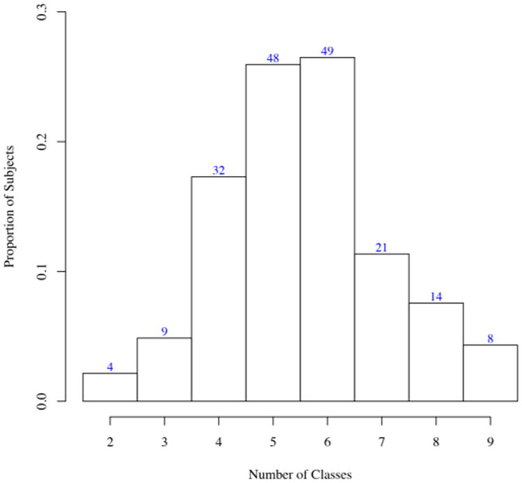
Number of latent classes of brain regions selected across 185 subjects from the ADHD-200 sample.

Figure 7.

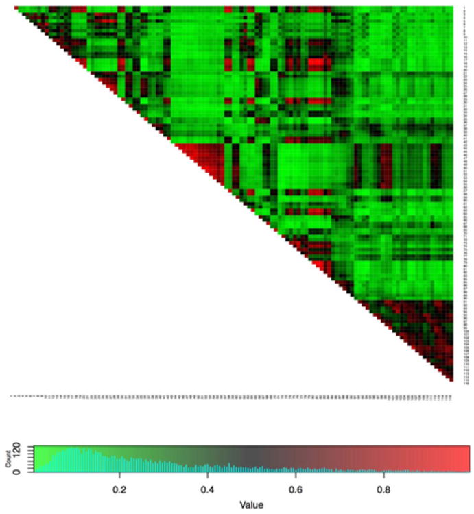
Overlap of the latent class structure across 185 subjects from the ADHD-200 sample. Each element of the matrix is the proportion of all 185 subjects in whom the corresponding two nodes fall in the same estimated latent class. The list of ROIs is given in Table 2 in the Appendix.

Figure 5.

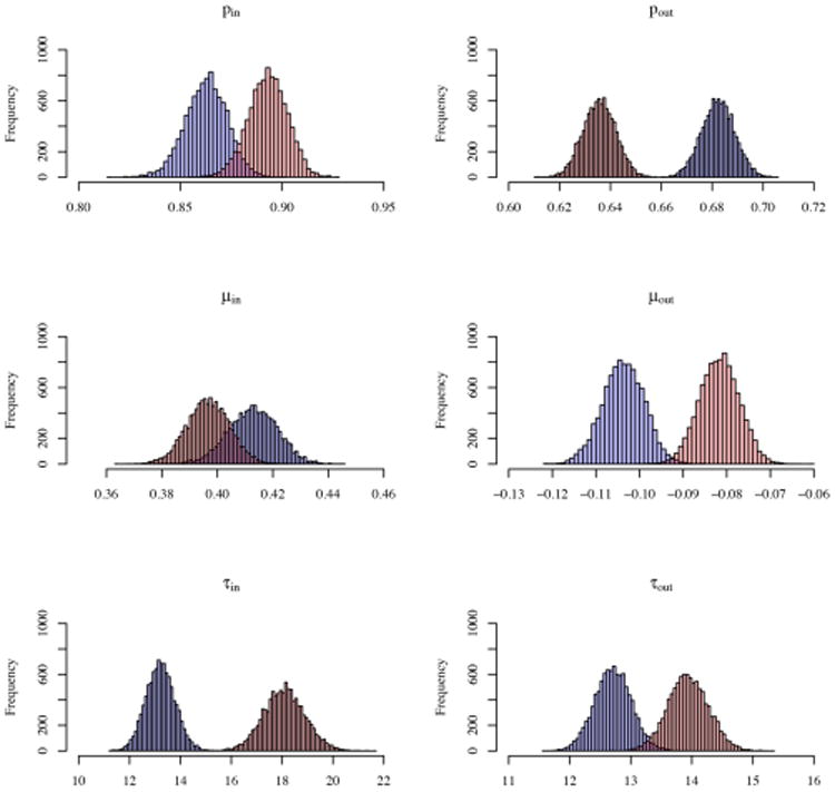
Posterior estimates of modularity parameters (Sparsity: p_in and p_out, edge weights: μ_in, μ_out, τ_in, τ_out) for subject 1 (Blue) and subject 2 (Red). First 100 samples were dropped, 9900 samples of each parameter shown.

5. Discussion

We have developed the weighted affiliation SBM as a Bayesian RGMM. Our RGMM utilizes an intuitive hierarchical parametric framework that accurately captures the affiliation community structure in simulated data. The benefits of using this fully Bayesian framework include incorporation of prior data, the ability to characterize the entirety of the posterior distribution, as well as the validity of estimates and accurate classification with smaller graphs. Additionally, this approach yields estimates of the modularity of the network as parameters in the model. For highly modular graphs, in which nodes in one latent class have considerably more connections and different weights as compared to nodes in different classes, our estimation method performs well with minimal misclassification and accurate estimates of the parameters.

Within the 185 functional brain networks from the ADHD-200 sample, subjects were estimated to have between 2 and 9 latent classes of brain regions, but considerable overlap in the latent structure is seen between some subjects. The commonalities between subjects appear to include some level of symmetry in the latent classes across the left and right hemispheres, as well as the functional overlap in the regions of the occipital lobe (see the red region near the center of the diagnoal of Figure 7) and several other groups of ROIs. While the SBM is unrealistic as a model of the true data-generating process in fMRI studies, it is nonetheless a useful and principled statistical tool for uncovering the large-scale structure in correlation between ROI time courses, which can help inform future studies in functional brain connectivity.

This framework allows the flexibility to utilize different distributions for the edge weights, detect overlapping communities, and estimate the community structure in directed graphs, all by straightforward alterations to the model. Current work is focused on extending this model to allow for groups of subjects that share a common structure, which appear plausible based on our analyses of the resting-state fMRI networks from the ADHD-200 sample. Additionally, we are working to incorporate regression and hypothesis testing to assess the differences in functional brain structure associated with changes in covariates.

APPENDIX A. ROI LABELS

Table 2. ROI labels for Figure 7 (From Left (1) to Right (116) and Top (1) to Bottom (116)).

Label	ROI
1	Precentral_L
2	Precentral_R
3	Frontal_Sup_L
4	Frontal_Sup_R
5	Frontal_Sup_Orb_L
6	Frontal_Sup_Orb_R
7	Frontal_Mid_L
8	Frontal_Mid_R
9	Frontal_Mid_Orb_L
10	Frontal_Mid_Orb_R
11	Frontal_Inf_Oper_L
12	Frontal_Inf_Oper_R
13	Frontal_Inf_Tri_L
14	Frontal_Inf_Tri_R
15	Frontal_Inf_Orb_L
16	Frontal_Inf_Orb_R
17	Rolandic_Oper_L
18	Rolandic_Oper_R
19	Supp_Motor_Area_L
20	Supp_Motor_Area_R
21	Olfactory_L
22	Olfactory_R
23	Frontal_Sup_Medial_L
24	Frontal_Sup_Medial_R
25	Frontal_Med_Orb_L
26	Frontal_Med_Orb_R
27	Rectus_L
28	Rectus_R
29	Insula_L
30	Insula_R
31	Cingulum_Ant_L
32	Cingulum_Ant_R
33	Cingulum_Mid_L
34	Cingulum_Mid_R
35	Cingulum_Post_L
36	Cingulum_Post_R
37	Hippocampus_L
38	Hippocampus_R
39	ParaHippocampal_L
40	ParaHippocampal_R
41	Amygdala_L
42	Amygdala_R
43	Calcarine_L
44	Calcarine_R
45	Cuneus_L
46	Cuneus_R
47	Lingual_L
48	Lingual_R
49	Occipital_Sup_L
50	Occipital_Sup_R
51	Occipital_Mid_L
52	Occipital_Mid_R
53	Occipital_Inf_L
54	Occipital_Inf_R
55	Fusiform_L
56	Fusiform_R
57	Postcentral_L
58	Postcentral_R
59	Parietal_Sup_L
60	Parietal_Sup_R
61	Parietal_Inf_L
62	Parietal_Inf_R
63	SupraMarginal_L
64	SupraMarginal_R
65	Angular_L
66	Angular_R
67	Precuneus_L
68	Precuneus_R
69	Paracentral_Lobule_L
70	Paracentral_Lobule_R
71	Caudate_L
72	Caudate_R
73	Putamen_L
74	Putamen_R
75	Pallidum_L
76	Pallidum_R
77	Thalamus_L
78	Thalamus_R
79	Heschl_L
80	Heschl_R
81	Temporal_Sup_L
82	Temporal_Sup_R
83	Temporal_Pole_Sup_L
84	Temporal_Pole_Sup_R
85	Temporal_Mid_L
86	Temporal_Mid_R
87	Temporal_Pole_Mid_L
88	Temporal_Pole_Mid_R
89	Temporal_Inf_L
90	Temporal_Inf_R
91	Cerebelum_Crus1_L
92	Cerebelum_Crus1_R
93	Cerebelum_Crus2_L
94	Cerebelum_Crus2_R
95	Cerebelum_3_L
96	Cerebelum_3_R
97	Cerebelum_4_5_L
98	Cerebelum_4_5_R
99	Cerebelum_6_L
100	Cerebelum_6_R
101	Cerebelum_7b_L
102	Cerebelum_7b_R
103	Cerebelum_8_L
104	Cerebelum_8_R
105	Cerebelum_9_L
106	Cerebelum_9_R
107	Cerebelum_10_L
108	Cerebelum_10_R
109	Vermis_1_2
110	Vermis_3
111	Vermis_4_5
112	Vermis_6
113	Vermis_7
114	Vermis_8
115	Vermis_9
116	Vermis_10

Appendix B. Distributions

Prior and sampling distributions are listed as follows: The latent class for each node i is distributed as

$$P(Z_i|\pi ,Q)={\pi }_1^{Z_{i1}}\cdots {\pi }_Q^{Z_{iQ}},P(\pi |Q)=\prod _{q=1}^Q{\pi }_q^{a_q-1}.$$

P(Y|Z, π, Q, θ, p) is given by

$$\begin{array}{c}\prod _{1<i<j<n}P(Y_{ij}|{\theta }_{\mathit{\text{in}}},{\theta }_{\mathit{\text{out}}},p_{\mathit{\text{in}}},p_{\mathit{\text{out}}},Z_i,Z_j,Q)\\ =\prod _{1<i<j<n}\prod _{q,l}P(Y_{ij}|{\theta }_{\mathit{\text{in}}},{\theta }_{\mathit{\text{out}}},p_{\mathit{\text{in}}},p_{\mathit{\text{out}}},Z_{iq}{Z}_{jl}=1,Q)\\ \prod _{1<i<j<n}\prod _{q=l}{[D_{\mathit{\text{in}}}(i,j)]}^{Z_{iq}{Z}_{jl}}\prod _{q\ne l}{[D_{\mathit{\text{out}}}(i,j)]}^{Z_{iq}{Z}_{jl}}\\ =\prod _A(P_{\mathit{\text{in}}}{(\frac{{\tau }_{\mathit{\text{in}}}}{2\pi })}^{1/2}exp\{-\frac{{\tau }_{\mathit{\text{in}}}}{2}{(Y_{ij}-{\mu }_{\mathit{\text{in}}})}^2\})\\ \prod _B(P_{\mathit{\text{out}}}{(\frac{{\tau }_{\mathit{\text{out}}}}{2\pi })}^{1/2}exp\{-\frac{{\tau }_{\mathit{\text{out}}}}{2}{(Y_{ij}-{\mu }_{\mathit{\text{out}}})}^2\})\\ \prod _C(1-p_{\mathit{\text{in}}})\prod _D(1-P_{\mathit{\text{out}}}),\end{array}$$

where

$$D_{\mathit{\text{in}}}(i,j)={(p_{\mathit{\text{in}}}{\left(\frac{{\tau }_{\mathit{\text{in}}}}{2\pi }\right)}^{1/2}exp\{-\frac{{\tau }_{\mathit{\text{in}}}}{2}{(Y_{ij}-{\mu }_{\mathit{\text{in}}})}^2\})}^{1(Y_{ij}\ne 0)}\times {(1-p_{\mathit{\text{in}}})}^{1(Y_{ij}=0)},$$

$$D_{\mathit{\text{out}}}(i,j)={(p_{\mathit{\text{out}}}{\left(\frac{{\tau }_{\mathit{\text{out}}}}{2\pi }\right)}^{1/2}exp\{-\frac{{\tau }_{\mathit{\text{out}}}}{2}{(Y_{ij}-{\mu }_{\mathit{\text{out}}})}^2\})}^{1(Y_{ij}\ne 0)}\times {(1-p_{\mathit{\text{out}}})}^{1(Y_{ij}=0)},$$

and A, B, C, and D satisfy

$$\begin{array}{c}A=\{i<j,q:Z_{iq}{Z}_{jq}=1,Y_{ij}\ne 0\},\\ B=\{i<j,q\ne l:Z_{iq}{Z}_{jl}=1,Y_{ij}\ne 0\},\\ C=\{i<j,q:Z_{iq}{Z}_{jq}=1,Y_{ij}=0\},\\ D=\{i<j,q\ne l:Z_{iq}{Z}_{jl}=1,Y_{ij}=0\}.\end{array}$$

Moreover, we set

$$\begin{array}{c}P(p_{\mathit{\text{in}}})=1(0<p_{\mathit{\text{in}}}<1),P(p_{\mathit{\text{out}}})=1(0<p_{\mathit{\text{out}}}<1),\\ p({\mu }_{\mathit{\text{in}}}|{\tau }_{\mathit{\text{in}}})={\left(\frac{{\tau }_{\mathit{\text{in}}}}{2\pi {\sigma }_{0,\mathit{\text{in}}}^2}\right)}^{1/2}exp\{\frac{{\tau }_{\mathit{\text{in}}}}{2\pi {\sigma }_{0,\mathit{\text{in}}}^2}{({\mu }_{\mathit{\text{in}}}-{\mu }_{0,\mathit{\text{in}}})}^2\},\\ P({\tau }_{\mathit{\text{in}}})={\beta }_{0,\mathit{\text{in}}}^{{\alpha }_{0,\mathit{\text{in}}}}\frac{1}{\mathrm{\Gamma }({\alpha }_{0,\mathit{\text{in}}})}{\tau }_{\mathit{\text{in}}}^{{\alpha }_{0,\mathit{\text{in}}}-1}exp\{-{\beta }_{0,\mathit{\text{in}}}{\tau }_{\mathit{\text{in}}}\},\\ P({\mu }_{\mathit{\text{out}}}|{\tau }_{\mathit{\text{out}}})={\left(\frac{{\tau }_{\mathit{\text{out}}}}{2\pi {\sigma }_{0,\mathit{\text{out}}}^2}\right)}^{1/2}exp\{\frac{{\tau }_{\mathit{\text{out}}}}{2{\sigma }_{0,\mathit{\text{out}}}^2}{({\mu }_{\mathit{\text{out}}}-{\mu }_{0,\mathit{\text{out}}})}^2\},\\ P({\tau }_{\mathit{\text{out}}})={\beta }_{0,\mathit{\text{out}}}^{{\alpha }_{0,\mathit{\text{out}}}}\frac{1}{\mathrm{\Gamma }({\alpha }_{0,\mathit{\text{out}}})}{\tau }_{\mathit{\text{out}}}^{{\alpha }_{0,\mathit{\text{out}}}-1}exp\{-{\beta }_{0,\mathit{\text{out}}}{\tau }_{\mathit{\text{out}}}\}.\end{array}$$

Then, the full conditional distributions are derived as follows:

First, we have

$$P(Z_i|\pi ,Q,p_{\mathit{\text{in}}},p_{\mathit{\text{out}}},\theta ,Y)\propto P(Y|\theta ,p,\pi ,Z,Q)P(Z_i|\pi ,Q)\alpha \prod _{1\le i\le j\le n}\prod _{q=l}{[D_{\mathit{\text{in}}}(i,j)]}^{Z_{iq}{Z}_{jl}}\prod _{q\ne l}{[D_{\mathit{\text{out}}}(i,j)]}^{Z_{iq}{Z}_{jl}}\times ({\pi }_1^{z_{il}}\cdots {\pi }_Q^{Z_{iQ}}).$$

Therefore, the full conditional distribution of Z_i given all others is proportional to

$$\prod _{q=1}^Q{\left[\prod _{j\ne i}{D}_{\mathit{\text{in}}}{(i,j)}^{Z_{jq}}{D}_{\mathit{\text{out}}}{(i,j)}^{\sum _{r\ne q}{Z}_{jr}}\right]}^{Z_{iq}}\times ({\pi }_1^{Z_{i1}}\cdots {\pi }_Q^{Z_{iQ}}),$$

Thus, we have Z_i| … ∼ Multinomial (π̂_i1,… π̂_iQ), where π̂_iq is given by

$${\stackrel{\sim }{\pi }}_{iq}=\frac{{\pi }_q\prod _{j\ne i}{D}_{\mathit{\text{in}}}{(i,j)}^{z_{jq}}{D}_{\mathit{\text{out}}}{(i,j)}^{\sum _{k\ne q}{Z}_{jk}}}{\sum _{q=1}^Q{\pi }_q\prod _{j\ne i}{D}_{\mathit{\text{in}}}{(i,j)}^{Z_{jq}}{D}_{\mathit{\text{out}}}{(i,j)}^{\sum _{k\ne q}{Z}_{jk}}}\text{for}q=1,\dots Q.$$

The full conditional distribution of π is given by

$$\begin{array}{cc}P(\pi |Q,Z,Y)& \propto P(Z|\pi ,Q)P(\pi |Q)\\ & \propto (\prod _{i=1}^n{\pi }_1^{Z_{i1}}\cdots {\pi }_Q^{Z_{iQ}})\left(\prod _{q=1}^Q{\pi }_q^{a_q-1}\right)\\ & \propto {\pi }_1^{\sum _{i=1}^n{Z}_{i1}+a_1-1}\cdots {\pi }_Q^{\sum _{i=1}^n{Z}_{iQ}+a_Q-1},\end{array}$$

which implies that

$$\pi |\dots ~\text{Dirichlet}(\sum _{i=1}^n{Z}_{i1}+a_1,\dots \sum _{i=1}^n{Z}_{iQ}+a_Q).$$

The full conditional distribution of p_in is given by

$$P(Y|\theta ,p,\pi ,Z,Q)P(p_{\mathit{\text{in}}})\propto p_{\mathit{\text{in}}}^{n_A}{(1-p_{\mathit{\text{in}}})}^{n_C}\cdot 1(0<p_{\mathit{\text{in}}}<1),$$

so p_in| … ∼ Beta(n_A + 1, n_C + 1), where n_A = |A| and n_B = |B|. Similarly, we have

$$P(p_{\mathit{\text{out}}}|\cdots )~\text{Beta}(n_B+1,n_D+1),$$

where n_C = |C| and n_D = |D|.

The full conditional distribution of μ_in is given by

$$\begin{array}{c}P({\mu }_{\mathit{\text{in}}}|\tau ,\pi ,Z,Q,p,Y)\propto P(Y|\theta ,p,\pi ,Z,Q)P({\mu }_{\mathit{\text{in}}}|{\tau }_{\mathit{\text{in}}}^{-1})\\ \propto exp\{\sum _A-\frac{{\tau }_{\mathit{\text{in}}}}{2}{(Y_{ij}-{\mu }_{\mathit{\text{in}}})}^2\}\\ \times exp\{-\frac{{\tau }_{\mathit{\text{in}}}}{2{\sigma }_{0,\mathit{\text{in}}}^2}{({\mu }_{\mathit{\text{in}}}-{\mu }_{0,\mathit{\text{in}}})}^2\},\end{array}$$

which implies that

$${\mu }_{\mathit{\text{in}}}|\cdots ~\mathrm{N}(\frac{{\sigma }_{0,\mathit{\text{in}}}^2\sum _A{Y}_{ij}+{\mu }_{0,\mathit{\text{in}}}}{n_A{\sigma }_{0,\mathit{\text{in}}}^2+1},\frac{{\sigma }_{0,\mathit{\text{in}}}^2{\tau }_{\mathit{\text{in}}}^{-1}}{n_A{\sigma }_{0,\mathit{\text{in}}}^2+1}).$$

Similarly, we have

$${\mu }_{\mathit{\text{out}}}|\cdots ~\mathrm{N}(\frac{{\sigma }_{0,\mathit{\text{out}}}^2\sum _B{Y}_{ij}+{\mu }_{0,\mathit{\text{out}}}}{n_A{\sigma }_{0,\mathit{\text{out}}}^2+1},\frac{{\sigma }_{0,\mathit{\text{out}}}^2{\tau }_{\mathit{\text{out}}}^{-1}}{n_A{\sigma }_{0,\mathit{\text{out}}}^2+1}).$$

The full conditional distribution of τ_in is given by

$$\begin{array}{c}P({\tau }_{\mathit{\text{in}}}|\mu ,\pi ,Z,Q,p,Y)\propto P(Y|\theta ,p,\pi ,Z,Q)\times P({\mu }_{\mathit{\text{in}}}|{\tau }_{\mathit{\text{in}}})P({\tau }_{\mathit{\text{in}}})\\ \propto \left[\prod _A\right(p_{\mathit{\text{in}}}{(\frac{{\tau }_{\mathit{\text{in}}}}{2\pi })}^{1/2}exp\{-\frac{{\tau }_{\mathit{\text{in}}}}{2}{(Y_{ij}-{\mu }_{\mathit{\text{in}}})}^2\}\left)\right]\\ \times {\left(\frac{{\tau }_{\mathit{\text{in}}}}{2\pi {\sigma }_{0,\mathit{\text{in}}}^2}\right)}^{1/2}exp\{\frac{{\tau }_{\mathit{\text{in}}}}{2{\sigma }_{0,\mathit{\text{in}}}^2}{({\mu }_{\mathit{\text{in}}}-{\mu }_{0,\mathit{\text{in}}})}^2\}\\ \times {\beta }_{0,\mathit{\text{in}}}^{{\alpha }_{0,\mathit{\text{in}}}}\frac{1}{\mathrm{\Gamma }({\alpha }_{0,\mathit{\text{in}}})}{\tau }_{\mathit{\text{in}}}^{{\alpha }_{0,\mathit{\text{in}}}-1}exp\{-{\beta }_{0,\mathit{\text{in}}}{\tau }_{\mathit{\text{in}}}\}\\ \propto {\tau }_{\mathit{\text{in}}}^{(\frac{n_A+1}{2}+{\alpha }_{0,\mathit{\text{in}}}-1)}exp\{\frac{-{\tau }_{\mathit{\text{in}}}}{2}\sum _A{(Y_{ij}-{\mu }_{\mathit{\text{in}}})}^2\}\times exp\{-\frac{{\tau }_{\mathit{\text{in}}}}{2{\sigma }_{0,\mathit{\text{in}}}^2}{({\mu }_{\mathit{\text{in}}}-{\mu }_{0,\mathit{\text{in}}})}^2-{\beta }_{0,\mathit{\text{in}}}{\tau }_{\mathit{\text{in}}}\},\end{array}$$

which implies that

$${\tau }_{\mathit{\text{in}}}|\cdots ~\text{Gamma}({\alpha }_{\mathit{\text{in}}}^{\ast },{\beta }_{\mathit{\text{in}}}^{\ast }),$$

where

$${\alpha }_{\mathit{\text{in}}}^{\ast }=\frac{n_A+1}{2}+{\alpha }_{0,\mathit{\text{in}}}$$

and

$${\beta }_{\mathit{\text{in}}}^{\ast }=\frac{1}{2}\sum _A{(Y_{ij}-{\mu }_{\mathit{\text{in}}})}^2+\frac{1}{2{\sigma }_{0,\mathit{\text{in}}}^2}{({\mu }_{\mathit{\text{in}}}-{\mu }_{0,\mathit{\text{in}}})}^2+{\beta }_{0,\mathit{\text{in}}}.$$

Similarly, we have

$${\tau }_{\mathit{\text{out}}}|\cdots ~\text{Gamma}({\alpha }_{\mathit{\text{out}}}^{\ast },),$$

with

$${\alpha }_{\mathit{\text{out}}}^{\ast }=\frac{n_B+1}{2}+{\alpha }_{0,\mathit{\text{out}}},$$

and

$${\beta }_{\mathit{\text{out}}}^{\ast }=\frac{1}{2}\sum _B{(Y_{ij}-{\mu }_{\mathit{\text{out}}})}^2+\frac{1}{2{\sigma }_{0,\mathit{\text{out}}}^2}{({\mu }_{\mathit{\text{out}}}-{\mu }_{0,\mathit{\text{out}}})}^2+{\beta }_{0,\mathit{\text{out}}}.$$

References

- 1.Aicher C, Jacobs AZ, Clauset A. Learning latent block structure in weighted networks. Journal of Complex Networks. 2015;3:221–248. [Google Scholar]
- 2.Ambroise C, Matias C. New consistent and asymptotically normal parameter estimates for random-graph mixture models. Journal of the Royal Statistical Society Series B. 2012;74:3–35. [Google Scholar]
- 3.Bullmore E, Sporns O. Complex brain networks: graph theoretical analysis of structural and functional systems. Nature Reviews Neuroscience. 2009;10:186–98. doi: 10.1038/nrn2575. [DOI] [PubMed] [Google Scholar]
- 4.Choi DS, Wolfe PJ, Airoldi EM. Stochastic blockmodels with a growing number of classes. Biometrika. 2012;99:273–284. doi: 10.1093/biomet/asr053. [DOI] [PMC free article] [PubMed] [Google Scholar]
- 5.Daudin JJ, Picard F, Robin S. A mixture model for random graphs. Statistics and Computing. 2008;18:173–183. [Google Scholar]
- 6.Erdös P, Rényi A. On random graphs I. Publ Math Debrecen. 1959;6:290–297. [Google Scholar]
- 7.Fortunato S. Community detection in graphs. Physics Reports. 2010;486:75–174. [Google Scholar]
- 8.Fortunato S, Barthélemy M. Resolution limit in community detection. Proceedings of the National Academy of Sciences of the United States of America. 2007;104:36–41. doi: 10.1073/pnas.0605965104. [DOI] [PMC free article] [PubMed] [Google Scholar]
- 9.Gao W, Zhu H, Giovanello KS, Smith JK, Shen D, Gilmore JH, Lin W. Evidence on the emergence of the brain's default network from 2-week-old to 2-year-old healthy pediatric subjects. Proceedings of the National Academy of Sciences. 2009;106:6790–6795. doi: 10.1073/pnas.0811221106. [DOI] [PMC free article] [PubMed] [Google Scholar]
- 10.Girvan M, Newman MEJ. Community structure in social and biological networks. Proceedings of the National Academy of Sciences of the United States of America. 2002;99:7821–7826. doi: 10.1073/pnas.122653799. [DOI] [PMC free article] [PubMed] [Google Scholar]
- 11.Hartigan JA, Wong MA. Algorithm AS 136: a k-means clustering algorithm. Journal of the Royal Statistical Society C. 1979;28:100–108. [Google Scholar]
- 12.Hofman JM, Wiggins CH. A Bayesian approach to network modularity. Physical Review Letters. 2008;100 doi: 10.1103/PhysRevLett.100.258701. [DOI] [PMC free article] [PubMed] [Google Scholar]
- 13.Hubert L, Arabie P. Comparing partitions. Journal of Classification. 1985;2:193–218. [Google Scholar]
- 14.Kolaczyk ED. Statistical Analysis of Network Data: Methods and Models. Springer Science+Business Media; 2009. [Google Scholar]
- 15.Lancichinetti A, Kivelä M, Saramäki J, Fortunato S. Characterizing the community structure of complex networks. PloS One. 2010;5:e11976. doi: 10.1371/journal.pone.0011976. [DOI] [PMC free article] [PubMed] [Google Scholar]
- 16.Lichtman JW, Pfister H, Shavit N. The big data challenges of connectomics. Nature Neuroscience. 2014;17:1448–1454. doi: 10.1038/nn.3837. [DOI] [PMC free article] [PubMed] [Google Scholar]
- 17.Mariadassou M, Robin S, Vacher C. Uncovering latent structure in valued graphs: a variational approach. Annals of Applied Statistics. 2010;4:715–742. [Google Scholar]
- 18.Matias C, Robin S. Modeling heterogeneity in random graphs: a selective review. arXiv preprint arXiv:1402.4296 2014 [Google Scholar]
- 19.Newman MEJ, Girvan M. Finding and evaluating community structure in networks. Physical Review E. 2004;69:16. doi: 10.1103/PhysRevE.69.026113. [DOI] [PubMed] [Google Scholar]
- 20.Nowicki K, Snijders TAB. Estimation and prediction for stochastic blockstructures. Journal of the American Statistical Association. 2001;96:1077–1087. [Google Scholar]
- 21.Peng L, Carvalho L. Bayesian degree-corrected stochastic blockmodels for community detection. arXiv preprint arXiv:1309.4796. 2013:1–23. [Google Scholar]
- 22.Plummer M, Best N, Cowles K, Vines K. CODA: convergence diagnosis and output analysis for MCMC. R News. 2006;6:7–11. [Google Scholar]
- 23.Reichardt J, Bornholdt S. Statistical mechanics of community detection. Physical Review E. 2006;74:16110. doi: 10.1103/PhysRevE.74.016110. [DOI] [PubMed] [Google Scholar]
- 24.Schweinberger M, Handcock MS. Local dependence in random graph models: characterisation, properties, and statistical inference. Journal of the Royal Statistical Society: Series B (Statistical Methodology) 2015;77:647–676. doi: 10.1111/rssb.12081. [DOI] [PMC free article] [PubMed] [Google Scholar]
- 25.Schweinberger M, Luna P. HERGM: hierarchical exponential-family random graph models. Journal of Statistical Software 2015 [Google Scholar]
- 26.Simpson SL, Bowman FD, Laurienti PJ. Analyzing complex functional brain networks: fusing statistics and network science to understand the brain. Statistics Surveys. 2013;7:1–36. doi: 10.1214/13-SS103. [DOI] [PMC free article] [PubMed] [Google Scholar]
- 27.Snijders TA. Statistical models for social networks. Annual Review of Sociology. 2011;37:131–153. [Google Scholar]
- 28.R Core Team. R: A Language and Environment for Statistical Computing. R Foundation for Statistical Computing; Vienna, Austria: 2015. [Google Scholar]
- 29.Traag VA, Bruggeman J. Community detection in networks with positive and negative links. Physical Review E – Statistical, Nonlinear, and Soft Matter Physics. 2009;80:7. doi: 10.1103/PhysRevE.80.036115. [DOI] [PubMed] [Google Scholar]
- 30.Tzourio-Mazoyer N, Landeau B, Papathanassiou D, Crivello F, Etard O, Delcroix N, Mazoyer B, Joliot M. Automated anatomical labeling of activations in SPM using a macroscopic anatomical parcellation of the MNI MRI single-subject brain. NeuroImage. 2002;15:273–289. doi: 10.1006/nimg.2001.0978. [DOI] [PubMed] [Google Scholar]
- 31.Vu DQ, Hunter DR, Schweinberger M. Model-based clustering of large networks. Annals of Applied Statistics. 2013;7:1010–1039. doi: 10.1214/12-AOAS617. [DOI] [PMC free article] [PubMed] [Google Scholar]
- 32.Xia M, Wang J, He Y. BrainNet Viewer: a network visualization tool for human brain connectomics. PloS One. 2013;8:e68910. doi: 10.1371/journal.pone.0068910. [DOI] [PMC free article] [PubMed] [Google Scholar]
- 33.Yang J, Leskovec J. Structure and overlaps of ground-truth communities in networks. ACM Transactions on Intelligent Systems and Technology. 2014;5:26. [Google Scholar]
- 34.Zhang Y, Friend AJ, Traud AL, Porter MA, Fowler JH, Mucha PJ. Community structure in congressional cosponsorship networks. Physica A: Statistical Mechanics and its Applications. 2008;387:1705–1712. [Google Scholar]