Rapid B-rep model preprocessing for immersogeometric analysis using analytic surfaces

Abstract

Computational fluid dynamics (CFD) simulations of flow over complex objects have been performed traditionally using fluid-domain meshes that conform to the shape of the object. However, creating shape conforming meshes for complicated geometries like automobiles require extensive geometry preprocessing. This process is usually tedious and requires modifying the geometry, including specialized operations such as defeaturing and filling of small gaps. Hsu et al. (2016) developed a novel immersogeometric fluid-flow method that does not require the generation of a boundary-fitted mesh for the fluid domain. However, their method used the NURBS parameterization of the surfaces for generating the surface quadrature points to enforce the boundary conditions, which required the B-rep model to be converted completely to NURBS before analysis can be performed. This conversion usually leads to poorly parameterized NURBS surfaces and can lead to poorly trimmed or missing surface features. In addition, converting simple geometries such as cylinders to NURBS imposes a performance penalty since these geometries have to be dealt with as rational splines. As a result, the geometry has to be inspected again after conversion to ensure analysis compatibility and can increase the computational cost. In this work, we have extended the immersogeometric method to generate surface quadrature points directly using analytic surfaces. We have developed quadrature rules for all four kinds of analytic surfaces: planes, cones, spheres, and toroids. We have also developed methods for performing adaptive quadrature on trimmed analytic surfaces. Since analytic surfaces have frequently been used for constructing solid models, this method is also faster to generate quadrature points on real-world geometries than using only NURBS surfaces. To assess the accuracy of the proposed method, we perform simulations of a benchmark problem of flow over a torpedo shape made of analytic surfaces and compare those to immersogeometric simulations of the same model with NURBS surfaces. We also compare the results of our immersogeometric method with those obtained using boundary-fitted CFD of a tessellated torpedo shape, and quantities of interest such as drag coefficient are in good agreement. Finally, we demonstrate the effectiveness of our immersogeometric method for high-fidelity industrial scale simulations by performing an aerodynamic analysis of a truck that has a large percentage of analytic surfaces. Using analytic surfaces over NURBS avoids unnecessary surface type conversion and significantly reduces model-preprocessing time, while providing the same accuracy for the aerodynamic quantities of interest.

1. Introduction

Immersogeometric analysis is a geometrically flexible technique for solving computational fluid–structure interaction (FSI) problems involving large, complex structural deformations (Kamensky et al., 2015; Hsu et al., 2014, 2015). This method was further investigated by Xu et al. (2016) in the context of a tetrahedral finite cell approach (Varduhn et al., 2016) for the simulation of incompressible flow (both laminar and turbulent) around geometrically complex objects. In immersogeometric analysis, a surface representation of a solid object is immersed into a non-boundary-fitted discretization of the background fluid domain. This background discretization is then used to solve for the flow physics using finite-element-based computational fluid dynamics (CFD). The main motivation behind the immersogeometric method is to alleviate the difficulties associated with mesh generation around complex geometries. Creating a boundary-fitted fluid-domain mesh that accurately captures all the features of the design geometry is often time consuming and labor intensive. Very often, small and thin geometric features are hard to discretize and, as a result, require extensive geometry cleanup, defeaturing, and mesh manipulation (Marcum & Gaither, 2000; Wang & Srinivasan, 2002; Beall et al., 2004; Lee et al., 2010). The immersogeometric method was proposed to eliminate these labor-intensive mesh generation procedures from the CFD simulation pipeline while still maintaining high accuracy of the simulation results. In addition, since the fluid domain is meshed independently and it is no longer necessary to defeature or remove small geometric features from the immersed object, the original design can be accurately preserved. The flexibility of the immersogeometric approach also allows it to be automated and placed in an optimization loop that searches for an optimal design (Wu et al., 2017).

Hsu et al. (2016) extended the immersogeometric method to directly use the boundary-representation (B-rep) of the CAD model to perform fluid flow simulations. Since, non-uniform rational B-splines (NURBS) are the de-facto surface representation used for representing the surfaces in B-rep, their method focused on using NURBS to perform the immersogeometric analysis. However, even though CAD models of aerodynamic and hydrodynamic structures have a large proportion of NURBS surfaces, CAD models of synthetic objects (such as road vehicles) usually have many flat features with rounded corners. These are represented internally in the CAD system using analytic surfaces rather than NURBS, since they can be easily manipulated by the solid modeling kernel and can be stored in a compact manner. Hanniel & Haller (2011) performed a detailed survey of over 3, 000 SolidWorks models and concluded that more than 90% of the B-rep surfaces were analytic surfaces. Converting these surfaces to NURBS in order to perform analysis usually leads to poorly parameterized NURBS surfaces and can lead to poorly trimmed or missing surface features. In addition, converting simple geometries such as cylinders to NURBS imposes a performance penalty since these geometries have to be dealt with as rational splines. As a result, the geometry has to be inspected again after conversion to ensure analysis compatibility and can increase the computational cost.

There are two main pre-processing steps required to perform immersogeometric analysis on complex CAD models. First, Gaussian quadrature information needs to be generated on the surface of the immersed model for the purpose of evaluating the weak Dirichlet boundary conditions (Bazilevs & Hughes, 2007). Second, the fluid-domain mesh with adequate refinement along the surfaces of the immersed object needs to be generated. In this paper, we have developed adaptive surface quadrature rules for the different analytic surfaces used in CAD models. We have also developed a mesh refinement technique that uses a hierarchical voxelization of the immersed model to generate an analysis-suitable fluid mesh.

The immersed objects used in previous immersogeometric methods were either made up of triangulated surfaces or trimmed NURBS surfaces. In the case of triangles, the Gaussian quadrature points were directly generated on the planar triangular surface. In the case of trimmed NURBS, the NURBS parameterization was used to generate the Gauss points. However, to generate the Gauss points on trimmed analytic surfaces, we need to develop surface quadrature rules for the trimmed analytic surfaces of the immersed B-rep models. In this paper, we have developed methods to generate Gaussian quadrature rules on trimmed analytic surfaces, including planes, cones, spheres, and toroids that are used in CAD models.

The boundary of solid models created using CAD systems is usually represented using multiple trimmed surfaces. In the case of parametric surfaces (NURBS), the parameterization is also used for storing the trim curves. In addition, the parametric space can be easily mapped to a normalized [0, 1] × [0, 1] domain, which makes the development of Gaussian quadrature rules straight forward. In addition, the normalized parametric domain can be easily subdivided using quad-tree techniques to generate adaptive surface quadrature rules for trimmed surfaces. In the case of analytic surfaces, the surface parameterization is not easily mapped to a normalized parametric domain, which complicates the development of adaptive surface quadrature rules. In this paper, we make use of 2D bounding boxes in the parametric space of the different analytic surfaces to generate adaptive surface quadrature rules.

In boundary-conforming fluid-flow analysis, the surface mesh of the immersed object can be directly used to generate the fluid-domain mesh. This surface mesh along with the growth parameter of an advancing-front volume mesh generation algorithm (Löhner & Parikh, 1988) can be used together to maintain a smaller mesh size closer to the surface of the immersed object, for the purpose of better resolving boundary layers. However, in immersogeometric analysis, the lack of a surface mesh complicates the generation of an adaptive fluid-domain mesh, which can lead to a mesh with a large number of elements that significantly increase the computational time. In this paper, we create a hierarchical voxelization of the immersed CAD model using GPU rendering techniques (Krishnamurthy et al., 2009a,b). We make use of this hierarchical voxelization to set the size parameters of the fluid-domain mesh generation algorithm. This method produces a mesh that has sufficiently small elements close to the immersed object boundary, while producing an overall fluid-domain mesh with fewer elements.

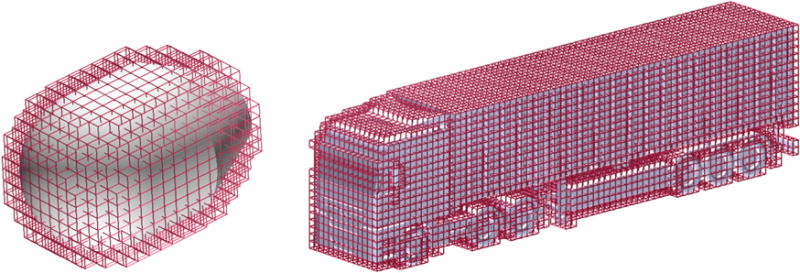
This paper is organized as follows. In Section 2, we briefly review the formulation for immersogeometric analysis. In Section 3, we discuss the surface quadrature rules for the different analytic surfaces. In Section 4, we explain the voxel-based method we use for generating the fluid-domain mesh with the required refinement around the surfaces of the immersed object. In Section 5, we apply our proposed method to the simulations of flow around a benchmark object made up of trimmed analytic surfaces, and a full-scale commercial truck (Fig. 1) to demonstrate the ability of our immersogeometric method for the aerodynamic analysis of industrial-scale simulations. In Section 6, we draw conclusions.

Figure 1.

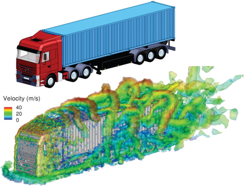
Top: The B-rep CAD model of a semi-trailer truck. The B-rep truck model consisting of analytic and NURBS surfaces is used directly to perform immersogeometric flow analysis. Bottom: Visualization of the instantaneous vortical structures of turbulent flow around the semi-trailer truck colored by velocity magnitude.

2. Immersogeometric fluid-flow analysis

The fundamentals of immersogeometric fluid-flow analysis consist of three main components. The flow physics is formulated using a variational multiscale (VMS) method for incompressible flows (Hughes et al., 2000; Bazilevs et al., 2007a). To capture the flow domain geometry accurately, adaptively refined quadrature rules are used in the intersected elements, without modifying the background mesh (Düster et al., 2008; Xu et al., 2016). Finally, the Dirichlet boundary conditions on the surface of the immersed objects are enforced weakly in the sense of Nitsche’s method (Nitsche, 1970; Bazilevs & Hughes, 2007). Here we briefly review this variationally consistent weak boundary conditions, which require the development of Gaussian quadrature rules for analytic surfaces.

The standard way of imposing Dirichlet boundary conditions is to enforce them strongly by ensuring that they are satisfied by all trial solution functions, which is not feasible in immersed methods. Instead, the strong enforcement is replaced by weakly enforced Dirichlet boundary conditions proposed by Bazilevs et al. (Bazilevs & Hughes, 2007; Bazilevs et al., 2007b, 2010). The semi-discrete problem can be stated as follows: Let Ω (subsets of ${ℝ}^d$, d ∈ {2, 3}) denote the spatial domain and Γ be its boundary. Consider a collection of disjoint elements {Ω^e}, ${\cup }_e{\mathrm{\Omega }}^e\subset {ℝ}^d$, with closures covering the fluid domain, $\mathrm{\Omega }\subset {\cup }_e\overline{{\mathrm{\Omega }}^e}$. Let ${\mathcal{V}}_u^h$ and ${\mathcal{V}}_p^h$ be the discrete velocity and pressure spaces of functions supported on these elements. Find fluid velocity ${\mathbf{u}}^h\in {\mathcal{V}}_u^h$ and pressure $p^h\in {\mathcal{V}}_p^h$ such that for all test functions ${\mathbf{w}}^h\in {\mathcal{V}}_u^h$ and $q^h\in {\mathcal{V}}_p^h$:

$$\begin{array}{l}{B}^{\mathrm{VMS}}\left(\{{\mathbf{w}}^h,q^h\},\{{\mathbf{u}}^h,q^h\}\right)-F^{\mathrm{VMS}}\left(\{{\mathbf{w}}^h,q^h\}\right)\\ -{\displaystyle {\int }_{{\mathrm{\Gamma }}^D}{\mathbf{w}}^h\cdot \left(-p^h\mathbf{n}+2\mu \mathit{\epsilon }({\mathbf{u}}^h)\mathbf{n}\right)d\mathrm{\Gamma }-}{\displaystyle {\int }_{{\mathrm{\Gamma }}^D}\left(2\mu \mathit{\epsilon }({\mathbf{w}}^h)\mathbf{n}+q^h\mathbf{n}\right)\cdot \left({\mathbf{u}}^h-\mathbf{g}\right)d\mathrm{\Gamma }}\\ -{\displaystyle {\int }_{{\mathrm{\Gamma }}^{D,-}}{\mathbf{w}}^h\cdot \rho \left({\mathbf{u}}^h\cdot \mathbf{n}\right)\left({\mathbf{u}}^h-g\right)d\mathrm{\Gamma }}\\ +{\displaystyle {\int }_{{\mathrm{\Gamma }}^D}{\tau }_{\mathrm{TAN}}^B\left({\mathbf{w}}^h-\left({\mathbf{w}}^h\cdot \mathbf{n}\right)\mathbf{n}\right)\cdot \left(\left({\mathbf{u}}^h-\mathbf{g}\right)-\left(\left({\mathbf{u}}^h-\mathbf{g}\right)\cdot \mathbf{n}\right)\mathbf{n}\right)d\mathrm{\Gamma }}\\ +{\displaystyle {\int }_{{\mathrm{\Gamma }}^D}{\tau }_{\mathrm{NOR}}^B\left({\mathbf{w}}^h\cdot \mathbf{n}\right)\left(\left({\mathbf{u}}^h-\mathbf{g}\right)\cdot \mathbf{n}\right)d\mathrm{\Gamma }}=0.\end{array}$$ (1)

In the above, B^VMS and F^VMS are the VMS discretization of the Navier–Stokes equations of incompressible flows. Their detailed expression is given by Xu et al. (2016). ρ is the density of the fluid, σ and ε are the stress and strain-rate tensors, respectively, n is the outward unit normal, Γ^D is the Dirichlet boundary that may cut through element interiors, Γ^D,− is the inflow part of Γ^D, on which u^h · n < 0, g is the prescribed velocity on Γ^D, and ${\tau }_{\mathrm{TAN}}^B$ and ${\tau }_{\mathrm{NOR}}^B$ are stabilization parameters that need to be chosen element-wise as a compromise between the conditioning of the stiffness matrix, variational consistency, and the stability of the formulation.

For immersogeometric methods, weakly enforced boundary conditions are particularly attractive as the additional Nitsche terms (the third to last terms on the left-hand side of Eq. (1)) are formulated independently of the mesh. In contrast to strong enforcement, which relies on boundary-fitted meshes to impose Dirichlet boundary conditions on the discrete solution space, the Nitsche terms also hold for intersected elements, where the domain boundary does not coincide with element boundaries. All that is needed is a separate discretization of the domain boundary with quadrature rules whose position of the quadrature points in intersected elements is known or can be determined. In Hsu et al. (2016), the geometry of the object was described entirely by NURBS. However, modern CAD models of synthetic objects tend to have many flat, conical, toroidal and spherical sections. These are represented internally in the CAD system using analytic surfaces rather than NURBS. Converting these features to NURBS usually leads to poor parameterization of NURBS surfaces, poorly trimmed or missing surface features, and the increase of computational cost. In this work, we tackle this issue by performing the surface integration of the weak boundary conditions directly using analytic surface information. This novel approach eliminates the need for converting to NURBS discretization for the object surface and allows the use of the native CAD model directly in immersogeometric analysis.

3. Adaptive surface quadrature for B-rep surfaces

In B-rep, a CAD solid model is represented using the set of faces that make up its boundary surfaces. The geometric descriptions of these faces can be categorized into two types: parametric and analytic surfaces. Generally, parametric surfaces are represented by NURBS surfaces, which have been used for immersogeoemtric applications previously (Hsu et al., 2016). Analytic surfaces—which include planes, cylinders, cones, spheres, and tori—are describe using algebraic equations (Fig. 2). Note that a cylindrical surface is considered a special case of a conical surface. We first review adaptive surface quadrature for NURBS in Section 3.1. The parameterization and the algebraic equations of analytic surfaces is presented in Section 3.2. The sub-cell based adaptive quadrature rules for these analytic surfaces is presented in Section 3.3.

Figure 2.

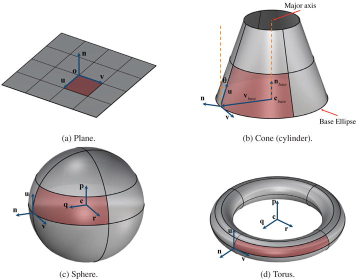
Analytic surfaces: plane, cone (cylinder), sphere, and torus. A sub-cell is red shaded for each analytic surface.

3.1. Surface quadrature for NURBS surfaces

The parameterization of an untrimmed NURBS surface is based on the tensor product of the knot locations along the u and v parametric directions. The tensor product parametric domain is usually divided at the knot locations to generate separate elements for the surface quadrature for each knot span. In the presence of trim curves, adaptive quadrature is required to better capture the geometry of the trimmed regions. Hsu et al. (2016) implemented adaptive quadrature by first dividing the base untrimmed NURBS surface patch into quadrature elements for each knot span. Then each Gauss point was tested whether it lies inside or outside the trimmed section of the NURBS surface. Only the Gauss points that lie inside the surfaces are kept. We extend this method to perform adaptive surface quadrature for analytic surfaces in this paper.

3.2. Surface quadrature for analytic surfaces

The algebraic equations for different types of analytic surfaces represent the mappings of a region of the uv parametric plane into the Euclidean three-dimensional space. An arbitrary 3D point of an analytic surface can be represented by a combination of the two parameters u and v in the algebraic equation. The region inside the parametric domain will be divided into quadrature elements for surface integrals.

3.2.1. Planar surface

For an untrimmed planar surface, the algebraic equation is

$$\mathbf{S}\left(u,v\right)=\mathbf{o}+u\mathbf{u}+v\mathbf{v},$$ (2)

where o is the origin of the plane and u and v are the basis vectors in a right-handed coordinate system (u, v, n). n is the normal vector of this planar surface and is defined as the cross product of the two basis vectors, u × v. For surface integrals, a sub-cell of a planar surface is based on the subsets of the real number domains along both u and v directions. A typical sub-cell of the planar surface is shown in Fig. 2a.

3.2.2. Conical and cylindrical surfaces

For an untrimmed conical surface, the algebraic equation is

$$\mathbf{S}\left(u,v\right)={\mathbf{c}}_{\text{base}}+\left(1+u\sin \theta /R\right){\mathbf{v}}_{\text{base}}\left(v\right)+u\cos \theta {\mathbf{n}}_{\text{base}},$$ (3)

where c_base is the base ellipse center, n_base is the unit vector in the normal direction of the base ellipse, R is the half length of the major axis of the base ellipse, and v_base(v) is the vector from the base ellipse center to the base ellipse point at a given value of v. Let u be the unit vector along the generator of the cone with parameter u increasing in the direction of n_base. The latitude metric u has a singular value if there is an apex. Let v be the unit vector along the base ellipse according to the right-hand rule around n_base. The longitude metric v has a domain [−π, π), which is periodic. The normal vector n of this conical surface is defined as −u × v. θ has the magnitude of the half angle of the cone. θ > 0 if u · v_base > 0 and θ < 0 if u · v_base < 0. θ has a domain between [−π/2, π/2). Note that the conical surface becomes a cylinder when θ = 0 and a planar surface when θ = −π/2. A typical sub-cell of a conical surface is shown in Fig. 2b.

3.2.3. Spherical surface

For an untrimmed spherical surface, the algebraic equation is

$$\mathbf{S}\left(u,v\right)=\mathbf{c}+r\sin u\mathbf{p}+r\cos u\left(\cos v\mathbf{q}+\sin v\mathbf{r}\right),$$ (4)

where c is the sphere center, r is the sphere radius, p is the unit vector in the direction from the south pole to the north pole, q is the unit vector in the direction from the center to the origin of the parametric space, and r = p × q. Let u be the unit vector along the longitude line of the sphere with parameter u defined as the angle between the vector from the center to the test point and the equatorial plane. The latitude metric u increases from the south pole to the north pole and has a domain between [−π/2, π/2). Let v be the unit vector along the latitude line of the sphere according to the right-hand rule around p. The longitude metric v has a domain between [−π, π), which is periodic. The normal vector n of this spherical surface is defined as −u × v. A typical sub-cell of a spherical surface is shown in Fig. 2c.

3.2.4. Toroidal surface

For an untrimmed toroidal surface, the algebraic equation is

$$\mathbf{S}\left(u,v\right)=\mathbf{c}+r\sin u\mathbf{p}+\left(R+r\cos u\right)\left(\cos v\mathbf{q}+\sin v\mathbf{r}\right),$$ (5)

where c is the torus center, r is the minor radius, R is the major radius, p is the unit vector along the torus axis, q is the unit vector in the direction from the center to the origin of the parametric space, and r = p × q. Let u be the unit vector along the poloidal direction of the torus with parameter u increasing in the direction of the axis p. u = 0 is the circle with the largest radius (R + r) relative to c. Let v be the unit vector along the toroidal direction of the torus according to the right-hand rule around p. Both the latitude metric u and the longitude metric v have the same domain between [−π, π), which are periodic. The normal vector n of this toroidal surface is defined as −u × v. A typical sub-cell of a toroidal surface is shown in Fig. 2d.

3.3. Sub-cell-based adaptive quadrature

To evaluate the quadrature points for a trimmed analytic surface, the untrimmed surface patch is evenly divided into patch elements along both parametric directions. The number of the quadrature patch elements is based on the physical Euclidean edge length along each parametric direction. Hence, the largest sub-cell will not exceed a user-defined element size. After the untrimmed domain is divided into patches, a three-point Gauss–Legendre quadrature rule in each parametric direction is used for the generation of the surface quadrature points in the parametric space for all of these surface patch elements. Note that the determinants of Jacobian for the quadrature points are evaluated directly using the ratio of the areas of the sub-cells in the physical and parametric spaces. In addition, patches that include degenerate points (such as the pole of a sphere or a cone vertex) need not be specifically handled, since the quadrature points are generated only on the interior of the analytic surface patches. The quadrature points are tested whether they lie inside the trimmed region of the surface. The inside quadrature points are used for the evaluation of the surface integral, while the outside quadrature points are discarded. This implementation of standard three-point Gaussian quadrature rules on a trimmed analytic surface is shown in Fig. 3.

Figure 3.

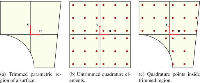
Standard Gaussian quadrature for a trimmed surface.

In order to accurately evaluate the surface integral of trimmed analytic surface, an adaptive quadrature method is implemented (Fig. 4). The patch elements that are intersected by a trim curve are identified and recursively refined. We make use of a 2D bounding box in the parametric domain to perform this refinement. First, the bounding box of a trim curve is checked whether it is fully inside or outside of the domain of a sub-cell, which is then used to exclude curve segments that are completely outside. The sub-cell domain that completely contains the bounding box of a trim curve segment is further refined. However, if the bounding box of the trim curve is not fully inside or outside of a sub-cell, a further test is required to ensure the trim curve is correctly intersected with the boundary of the sub-cell. We check the total number of the intersection points between all the trim curves and sub-cell boundary. If there exists at least two intersection points, the sub-cell is recursively refined.

Figure 4.

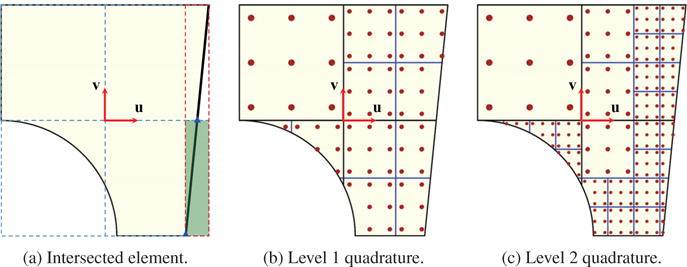
Sub-cell-based adaptive quadrature is used for a better evaluation of the surface integral of a trimmed surface.

Fig. 4a shows an example case for finding an intersected patch element (marked in green) that needs to be sub-divided. First, the bounding-box of the trim-curve (marked in red) is found to be intersecting with the bottom-right sub-cell patch element. Next, the number of intersection points between the sub-cell boundary and the trim curves are calculated. In this example, there are two intersection points (marked in blue triangles). Hence, this sub-cell is subdivided into 4 sub-cells. This process is recursively performed until a user-defined subdivision level is reached. Fig. 4b and 4c show the results of two different levels of recursive subdivision for a trimmed patch.

3.4. Implementation

We use SolidWorks and ACIS solid modeling kernel to efficiently generate the surface quadrature points directly from B-rep models. SolidWorks is a widely used CAD software and ACIS is a commercial CAD modeling kernel. The ACIS kernel includes methods that can be used to read and interpret the equations of an analytic surface. The software implementation of the generation of sub-cell-based adaptive quadrature points on analytic surfaces is shown in Fig. 5.

Figure 5.

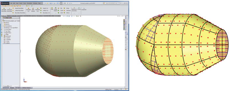
SolidWorks plug-in for generating surface quadrature rules directly from a B-rep model using ACIS kernel. The surface parameterization of the object is shown on the right.

4. Voxel-based non-boundary-fitted mesh generation

The mesh for the fluid domain needs to be suitably refined near the surfaces of the immersed object in order to accurately capture the flow in the boundary layer surrounding the object. For traditional boundary-fitted mesh generation, the surface tessellation can be used to control the size of the mesh in the region close to the surface. However, in immersogeometric analysis, since the immersed object is not tessellated, the size of the immersed mesh needs to be controlled using other methods. In this work, we use a voxel-based approach for controlling the size of the fluid-domain mesh near the surfaces of the immersed object. The voxels are considered as individual axis-aligned bounding-boxes (AABBs) that can be used to set the maximum mesh sizes for the tetrahedral fluid-domain mesh.

We make use of a rendering-based voxelization method (Krishnamurthy et al., 2009a; Hsu et al., 2016) to create voxelizations of different user-defined resolutions of the immersed object using the GPU. The analytic surfaces of the immersed model are converted into triangles with a very fine resolution that is less than one-tenth of the resolution of the immersed mesh. The time taken to perform the classification is the sum of the time taken to evaluate the analytic surfaces in the model and the total time taken to render each slice for classification. For example, the total time taken to evaluate the analytic surfaces in the finest model of the torpedo shape in Section 5.2 is 0.06 second, while the time taken to classify the 778,284,864 (1204 × 804 × 804) voxels is 28.83 seconds. These timings are obtained by running our classification algorithm on a MacBook Pro with a 2.7 GHz processor, 16 GB RAM, and an NVIDIA GeForce GT 650M GPU.

For the generation of the non-boundary-fitted tetrahedral mesh, the boundary voxels of a coarse voxelization of the CAD model are used for the local refinement. The boundary voxels are identified based on whether there are surface Gauss points inside them. The boundary voxels specify the regions that are near the immersed boundary where sufficient local refinement is needed to accurately capture the fluid boundary layer. To implement this method, we use the functionality of “SizeBox” in ANSA, which is a commercial mesh generator. In ANSA, this function constrains the maximum length of the tetrahedral elements within each SizeBox. The 3D tetrahedral mesh is generated using the “TetraCFD” mesh generation algorithm, which is based on the advancing-front mesh-generation method (Löhner & Parikh, 1988).

A visualization of the boundary voxels used in one of our B-rep test models (torpedo) is shown on the left in Fig. 6; this particular torpedo model has 734 boundary voxels. Since the SizeBox will only constrain the maximum length of the tetrahedral elements that are fully inside the AABB of the boundary voxel, the dimension of SizeBox should be larger than the element size near the immersed object. The non-boundary-fitted tetrahedral mesh using these boundary voxels is shown later in Fig. 9b. The element size near the object surfaces is 0.04, while the voxel dimension is 0.1, which is 2.5 times larger. The tetrahedral elements, which are arbitrarily intersected with the immersed body, are sufficiently refined within each voxel. This locally refined non-boundary-fitted mesh is suitable for immersogeometric fluid-flow analysis.

Figure 6.

Visualization of a coarse voxelization of the CAD models used for local refinement of the immersed mesh. A fine voxelization is used for point membership classification.

Figure 9.

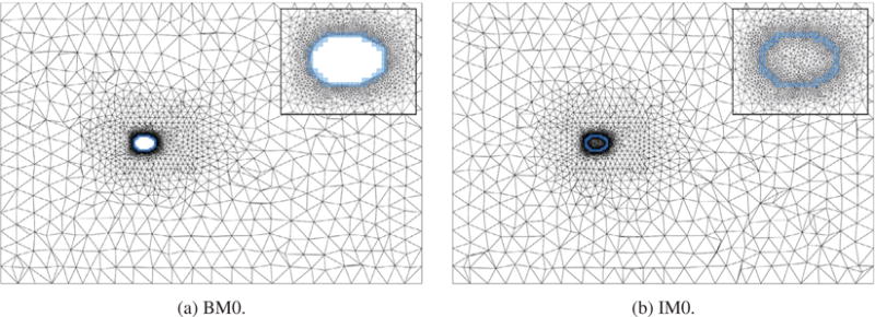
Central cross-section of the coarsest boundary-fitted mesh (BM0) and the coarsest immersogeometric mesh (IM0).

5. B-rep immersogeometric analysis with analytic surfaces

In this section, the B-rep-based immersogeometric analysis with analytic surfaces is used to simulate the fluid flow around bluff bodies. First, we show the immersogeometric analysis of the flow around an untrimmed analytic spherical surface to compare the results with a previous study using an untrimmed NURBS sphere (Hsu et al., 2016). Second, we simulate the flow around a torpedo shaped object with trimmed analytic surfaces and compare it with both a NURBS-based immersogeometric example and a boundary-fitted fluid-flow example that is used as a reference. Finally, the flow past a B-rep CAD model of a full-scale semi-trailer truck with many analytic surfaces is simulated to demonstrate the accuracy and efficiency of the immersogeometric method with analytic surfaces.

5.1. Benchmark: Flow around an untrimmed analytic spherical surface

The flow around an untrimmed spherical surface at Reynolds number (Re) 100 is used as a benchmark to assess the accuracy of our analytic surface-based immersogeometric method. The simulation setup including the computational domain and the boundary conditions used is identical to those used in Xu et al. (2016). An untrimmed spherical surface is immersed into a linear tetrahedral background fluid mesh “IM1”. In addition, two adaptive quadrature levels are used for the analytic surfaces to faithfully capture the geometry in the intersected background elements of the fluid mesh.

To investigate the required surface quadrature density for the flow around an analytic spherical surface, we consider different levels of surface quadrature patch refinement (same as Hsu et al. (2016)). A three-point Gauss–Legendre quadrature rule in each parametric direction is applied to the quadrature elements¹. However, the patch subdivision for the analytic surface into quadrature elements is different from that of the NURBS parameterization used for the sphere. The subdivision of the analytic surface is based on the uniform length scale in physical space, while the division of the NURBS sphere in Hsu et al. (2016) is based on uniform knot spans, which in practice do not yield a uniform length in physical space (Hughes et al., 2005, Appendix B). Fig. 7 shows three levels of surface quadrature element refinement on both analytic (red lines) and NURBS (blue lines) surfaces.

Figure 7.

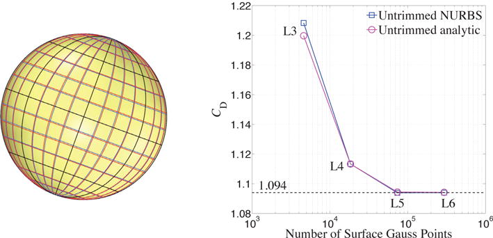
Comparison between analytic (red lines) and NURBS (blue lines) surfaces with three levels of surface quadrature element refinement. Convergence of the Drag coefficient with surface quadrature refinement. The drag coefficients converge to 1.094.

The results of the drag coefficient C_D for the analytic spherical surface and the NURBS surface for different levels of surface quadrature refinement (Level 3 to Level 6) are shown in Fig. 7. The results demonstrate that the density and distribution of the surface quadrature points are crucial for the weak enforcement of Dirichlet boundary conditions and for obtaining accurate flow solutions.

5.2. Benchmark: Flow around an object with trimmed analytic surfaces

In this section, we simulate the flow around a torpedo shaped object with a combination of trimmed and untrimmed analytic surfaces to assess the accuracy of our analytic-surface-based immersogeometric method. The torpedo shaped object consists of one trimmed spherical surface, one untrimmed cylindrical surface, one untrimmed conical surface, and one trimmed planar surface (Fig. 5). The dimensions of the object are shown in Fig. 8a. The same object is converted to NURBS and immersed in the same background meshes used for the analytic surfaces for the comparison of the two immersogeometric approaches. In addition, a boundary-fitted tetrahedral-mesh-based CFD is simulated as a reference.

Figure 8.

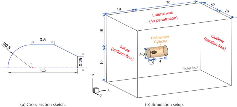
Left: Dimensions of the torpedo shaped object. Right: Computational domain, refinement cylinder, boundary conditions, and the immersed object.

The simulation setup including the dimensions of the computational domain, the refinement cylinder, and the boundary conditions is shown in Fig. 8b. All sizes are non-dimensional. The inflow velocity and the fluid density are set to be unity. The characteristic length is chosen as the diameter of the front hemisphere and thus the Reynolds number can be defined as the inverse of the viscosity, that is, Re = μ⁻¹. In our simulations, the viscosity is set to 0.01, so the flow around this object is at Re = 100. The no-slip boundary condition is enforced weakly at the surfaces of the object.

The mesh resolution near the surfaces of the object is critical to resolving the boundary layers accurately. For this object, we discretize the fluid domain using linear tetrahedral elements, due to their capability of efficiently generating a locally refined non-boundary-fitted mesh around a complex object. Using the mesh generation method proposed in Section 4, the boundary voxels are used to define the locations for local refinement. To have a fair comparison, the same refinement strategy is also applied to the boundary-fitted mesh. The detailed mesh statistics and the characteristic element sizes used in the four sets of boundary-fitted meshes (BM0, BM1, BM2, and BM3) and immersogeometric meshes (IM0, IM1, IM2, and IM3) are listed in Tables 1 and 2, respectively. The central cross-section of the two coarsest meshes (BM0 and IM0) are shown in Fig. 9. The difference in the number of elements in the respective boundary-fitted and immersed meshes is less than 4%, making them comparable for the simulations. In the BM0 and IM0 setup, the boundary voxels for Level 0 (blue) are used to set the mesh size near the surfaces of the object (Fig. 10a). In the BM1 and IM1 setup, the boundary voxels for both Level 0 (blue) and Level 1 (green) are used to set the mesh size near the surfaces of the object (Fig. 10b). In general, for a Level n setup, the boundary voxels of all levels until n are used to set the mesh size near the surfaces of the object. Detailed listings of the different voxel sizes used for the local refinement for the four cases is given in Table 3.

Table 1.

Element sizes and C_D in the boundary-fitted mesh around an object.

Mesh	Total number of elements	Near object element size	Refinement cylinder element size	Outer box element size	CD
BM0	277,996	0.04	0.4	1.4	1.197
BM1	911,371	0.02	0.2	1.2	1.190
BM2	3,453,690	0.01	0.1	1.0	1.186
BM3	15,731,430	0.005	0.05	0.8	1.185

Table 2.

Element sizes and drag coefficients in the immersogeometric mesh around an object.

Mesh	Effective number of elements	Near object element size	Refinement cylinder element size	Outer box element size	CD Analytic	CD NURBS
IM0	277,493	0.04	0.4	1.4	1.211	1.210
IM1	883,216	0.02	0.2	1.2	1.194	1.194
IM2	3,317,197	0.01	0.1	1.0	1.187	1.187
IM3	15,174,511	0.005	0.05	0.8	1.185	1.185

Figure 10.

Central cross-section of the immersogeometric mesh IM0 and IM1.

Table 3.

Voxel-based SizeBox used in the mesh refinement around the object.

Mesh	Voxel size (element size) Level 0	Voxel size (element size) Level 1	Voxel size (element size) Level 2	Voxel size (element size) Level 3
IM0/BM0	0.1 (0.04)	–	–	–
IM1/BM1	0.1 (0.04)	0.05 (0.02)	–	–
IM2/BM2	0.1 (0.04)	0.05 (0.02)	0.025 (0.01)	–
IM3/BM3	0.1 (0.04)	0.05 (0.02)	0.025 (0.01)	0.0125 (0.005)

In this work, we again use sub-cell-based adaptive quadrature to handle the intersected tetrahedral elements for the immersogeometric meshes. As shown in Xu et al. (2016), two levels of adaptive quadrature provide a reasonable balance between the accuracy and computational cost for the immersogeometric analysis. Meanwhile, as shown in Hsu et al. (2016), setting the surface patch element size the same as the volume element size near the object can ensure sufficient surface quadrature point density for the immersogeometric flow analysis of trimmed patches. The maximum quadrature patch element sizes used in all the cases are the same as their corresponding tetrahedral element sizes near the object.

All simulations are performed with a time-step size of 0.01. In each case, the simulation is continued until the steady state is reached. Fig. 11 shows that the drag coefficients C_D for both the boundary-fitted and the analytic-surface-based immersogeometric analysis converge to 1.185 using the finest meshes. The numerical values of the drag coefficients for the two cases are also listed in Tables 1 and 2, respectively. The velocity magnitude contours for these two cases are compared in Fig. 12 to demonstrate the quality of the flow solution.

Figure 11.

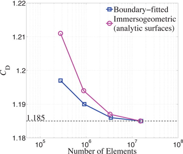
Drag coefficient convergence associated with number of effective fluid elements for boundary-fitted and immersogeometric (analytic surfaces) cases. The drag coefficients converge to 1.185.

Figure 12.

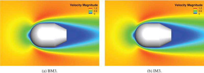
Velocity magnitude contours of the boundary-fitted and the immersogeometric simulation results.

Note that for the immersogeometric cases, the difference in the drag coefficients using the analytic surfaces and the NURBS surfaces is less than 0.001 for all levels of mesh refinement. However, as shown in Fig. 13, the time taken to evaluate the surface Gauss points for the analytic surfaces is approximately 3 times faster than that of the NURBS surfaces.

Figure 13.

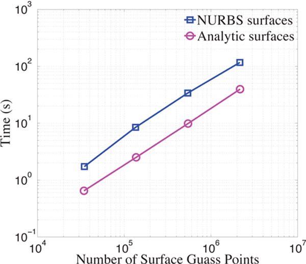
Time costs of the surface Gauss points evaluation for the NURBS surfaces and the analytic surfaces.

These results demonstrate that using trimmed analytic surfaces for immersogeometric fluid-flow analysis, with surface quadrature rules generated using the method proposed in Section 3.4, produces accurate prediction of flow quantities of interest and is more efficient than using only NURBS surfaces.

5.3. Airflow around a semi-trailer truck

In order to demonstrate the applicability of our analytic-surface-based immersogeometric method to industrial scale problems, we simulate the flow past a full-scale semi-trailer truck. To perform the CFD analysis of flow around a complex model, a common practice is to preprocess the B-rep by tessellating it into a triangular mesh (Xu et al., 2016) or convert it to NURBS (Hsu et al., 2016). However, both these methods are not ideal and can lead to time-consuming mesh generation or unnecessary conversion to parametric surfaces (e.g. NURBS). The conversion to NURBS may also result in poorly parameterized NURBS surfaces and often leads to poorly trimmed or missing surface features. In addition, the time cost for generating the surface quadrature for NURBS surfaces is generally higher than that for the analytic surfaces. Therefore, directly using the analytic surfaces from the B-rep model is an ideal solution to integrate design and analysis.

In a solid CAD model, analytic surfaces have frequently been used for B-rep model construction. A typical B-rep model of a road vehicle like the semi-trailer truck shown in Fig. 1 has a larger number of analytic surfaces than parametric surfaces. This particular model has only 8 parametric surfaces but 2,480 analytic surfaces, which include 1,769 planar surfaces, 689 conical and cylindrical surfaces, 8 spherical surfaces, and 14 toroidal surfaces. Specifically, the tire mainly consists of cylindrical surfaces, the boundary of the trailer includes many planar surfaces, and the corner of the mirror bracket is a toroidal surface.

There is a significant advantage of using analytic surfaces over NURBS for generating the surface quadrature points. For this semi-trailer truck, it takes only 15.54 s for generating 497,552 Gauss points using analytic surfaces, while it takes 44.12 s for generating 496,096 Gauss points when all surfaces are converted to NURBS. Using analytic surfaces, generating the surface Gaussian quadrature points is nearly 3 times faster than using NURBS. In addition, for the NURBS case, there is an additional step of converting the analytic surfaces to the NURBS surfaces. Therefore, using the analytic surfaces directly for generating the Gaussian quadrature points enables us to more efficiently preprocess the model.

The dimensions of the truck and its simulation setup including the computational domain and boundary conditions are shown in Fig. 14. A uniform inflow with a streamwise velocity of 31.293 m/s (70 mph), which corresponds to a typical driving speed of the semi-trailer truck on highways, is applied. A no-slip boundary condition is applied to the ground for simplicity. The density and the dynamic viscosity of the air are 1.177 kg/m³ and 1.846 × 10⁻⁵ kg/(m·s), respectively. As in Englar (2001), the characteristic length of the truck is defined as the length of the truck along the inflow direction, which is 15.083 m in our case. The Reynolds number is around 30 million which yields a highly turbulent flow.

Figure 14.

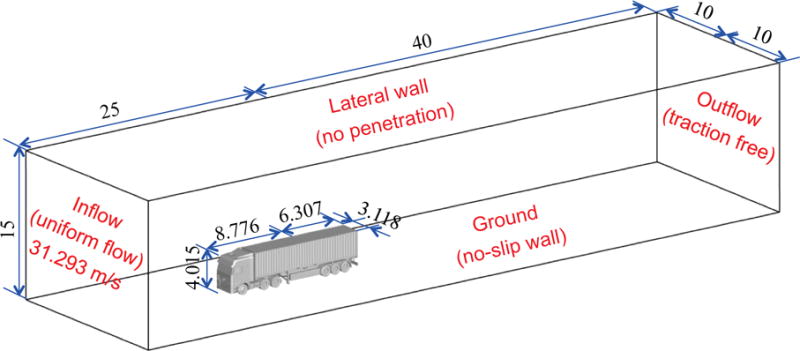
Dimensions of the immersed semi-trailer truck and the boundary conditions of the flow domain.

The B-rep model of this semi-trailer truck is directly immersed into the tetrahedral background mesh. The boundary voxels for the local mesh refinement of this semi-trailer truck are shown in Fig. 6. The voxel-based SizeBox, three refinement zones and the immersogeometric mesh are shown in Fig. 15. The element sizes set for the fluid domain boundaries, outer refinement zone, inner refinement zone, object bounding-box zone and the voxels are 2.0 m, 1.0 m, 0.5 m, 0.2 m and 0.1 m, respectively. This immersogeometric mesh consists of 2,007,309 linear tetrahedral elements (1,556,810 effective elements in the fluid domain). Two levels of adaptive quadrature is used in the intersected background elements to accurately integrate the volume integrals and faithfully capture the geometry of the semi-trailer truck. The inside-outside classification of the volume quadrature points is carried out using the finest level of the voxelization. In this case, the finest voxelization consists of 12,369,920 (128 × 160 × 604) voxels; the size of each voxel (0.025 m) is 4 times smaller than the near object element size (0.1 m).

Figure 15.

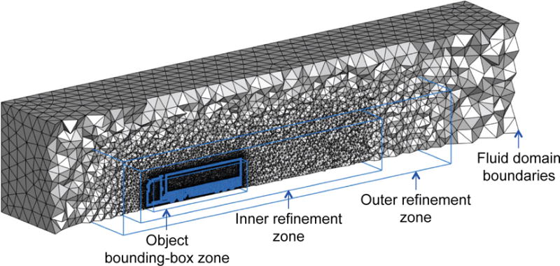
Locally refined tetrahedral meshes of the fluid domain for aerodynamic analysis of the semi-trailer truck. We show the mesh cut along a plane in flow direction. The B-rep model is used directly for generating the boundary voxels for the local mesh refinement.

The instantaneous vortical structures of the highly turbulent flow around the semi-trailer truck (Fig. 1) is visualized using the isosurfaces of λ₂ = −100, −200, and −400. λ₂ is the second largest eigenvalue of the tensor S² + Ω², where S and Ω are the symmetric and antisymmetric components of ∇u, respectively. The vortex core is defined as the region where λ₂ < 0 (see Jeong & Hussain (1995) for details). We also compute the time-averaged drag coefficient ${\overline{C}}_{\mathrm{D}}=2{\overline{F}}_{\mathrm{D}/\rho }{U}^{2}A$, where U is the inflow velocity, ${\overline{F}}_{\mathrm{D}}$ is the time-averaged drag force, and A = 9.703 m² is the area of the frontal truck surface projected onto a plane perpendicular to the main flow direction. The values of ${\overline{C}}_{\mathrm{D}}$ are 0.735 and 0.728 for the B-rep case with analytic surfaces and the case with only NURBS surfaces, respectively. These values are computed by simulating the flow for 18 s with a time-step size of 0.001 s. The drag coefficients are in good agreement with the reference drag coefficients of heavy vehicles, which are in the range of 0.6–0.9 (Götz & Mayr, 1998; Englar, 2001; Chowdhury et al., 2013). The time-averaged velocity and pressure fields in a planar cross-section are shown in Fig. 16.

Figure 16.

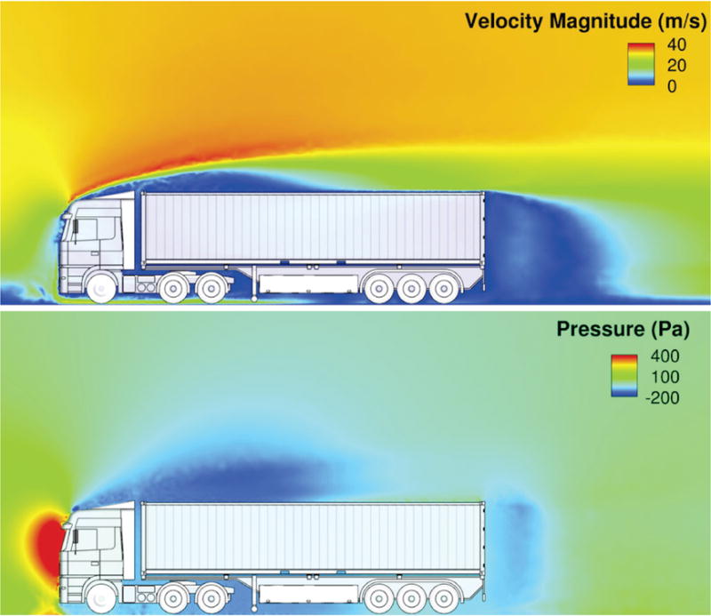
Time-averaged velocity (top) and pressure (bottom) fields on a planar cut for the case with analytic surfaces.

The study of the semi-trailer truck presented in this section demonstrates an effective way to perform industrial-scale turbulent flow simulations using our B-rep-based immersogeometric flow analysis. The proposed method is an efficient way to overcome the complicated mesh generation process and maintain a high solution accuracy for the flow around a complex real-world geometry.

6. Conclusions

We have presented a new method for immersogeometric fluid-flow analysis that directly uses CAD models with analytic surfaces. Solid models of complex objects usually consist of many analytic surfaces. Our method directly uses the analytic surface equations to generate the surface Gaussian quadrature points. We have also extended our methods to perform adaptive quadrature on trimmed analytic surfaces. Our method does not require converting the B-rep CAD model surfaces to NURBS, which is computationally expensive and can lead to poorly parameterized or converted surfaces. In addition, the method avoids the challenges associated with geometry cleanup and mesh generation. We have also presented a method to generate a fluid-domain mesh with selective refinement around the surfaces of the immersed object using hierarchical voxelization of the object. Our timing results show that our analytic-surface-based method is much faster in computing the Gauss point information than using only NURBS surfaces. In addition, the flow simulation results obtained using immersogeometric analytic surfaces are in good agreement with reference flow simulation results obtained using NURBS and boundary-fitted CFD. Finally, the analytic-surface-based immersogeometric method can be easily applied to industrial-scale flow analysis. In our simulation of flow past the semi-trailer truck, we directly used the CAD model generated using SolidWorks to perform immersogeometric analysis. The drag coefficient computed using the immersogeometric method is in good agreement with the values of drag coefficient of similar semi-trail trucks reported in the literature.

Highlights.

• Fast preprocessing of B-rep models for immersogeometric fluid-flow analysis.

• Directly use analytic surfaces of B-rep CAD models without conversion to NURBS.

• Generation of surface integration points directly on analytic surfaces.

• Adaptive mesh refinement near analytic surfaces using voxelization.

References

- ACIS. 2017 https://www.spatial.com/products/3d-acis-modeling. [Accessed 21 January 2017]
- ANSA. 2017 http://www.beta-cae.com/ansa.htm. [Accessed 21 January 2017]
- Bazilevs Y, Calo VM, Cottrel JA, Hughes TJR, Reali A, Scovazzi G. Variational multiscale residual-based turbulence modeling for large eddy simulation of incompressible flows. Computer Methods in Applied Mechanics and Engineering. 2007a;197:173–201. [Google Scholar]
- Bazilevs Y, Hughes TJR. Weak imposition of Dirichlet boundary conditions in fluid mechanics. Computers & Fluids. 2007;36:12–26. [Google Scholar]
- Bazilevs Y, Michler C, Calo VM, Hughes TJR. Weak Dirichlet boundary conditions for wall-bounded turbulent flows. Computer Methods in Applied Mechanics and Engineering. 2007b;196:4853–4862. [Google Scholar]
- Bazilevs Y, Michler C, Calo VM, Hughes TJR. Isogeometric variational multiscale modeling of wall-bounded turbulent flows with weakly enforced boundary conditions on unstretched meshes. Computer Methods in Applied Mechanics and Engineering. 2010;199:780–790. [Google Scholar]
- Beall MW, Walsh J, Shephard MS. A comparison of techniques for geometry access related to mesh generation. Engineering with Computers. 2004;20:210–221. [Google Scholar]
- Chowdhury H, Moria H, Ali A, Khan I, Alam F, W S. A study on aerodynamic drag of a semi-trailer truck. Procedia Engineering. 2013;56:201–205. [Google Scholar]
- Düster A, Parvizian J, Yang Z, Rank E. The finite cell method for three-dimensional problems of solid mechanics. Computer Methods in Applied Mechanics and Engineering. 2008;197:3768–3782. [Google Scholar]
- Englar RJ. Advanced Aerodynamic Devices to Improve the Performance, Economics, Handling and Safety of Heavy Vehicles. 2001 SAE Technical Paper 2001-01-2072 SAE International. [Google Scholar]
- Götz H, Mayr G. Commercial vehicles. In: Hucho W, editor. Aerodynamics of Road Vehicles: From fluid mechanics to vehicle engineering. 4th. Society of Automotive Engineers; 1998. pp. 415–488. chapter 9. [Google Scholar]
- Hanniel I, Haller K. 12th International Conference on Computer-Aided Design and Computer Graphics. IEEE; 2011. Direct rendering of solid CAD models on the GPU; pp. 25–32. [Google Scholar]
- Hsu MC, Kamensky D, Bazilevs Y, Sacks MS, Hughes TJR. Fluid–structure interaction analysis of bioprosthetic heart valves: Significance of arterial wall deformation. Computational Mechanics. 2014;54:1055–1071. doi: 10.1007/s00466-014-1059-4. [DOI] [PMC free article] [PubMed] [Google Scholar]
- Hsu MC, Kamensky D, Xu F, Kiendl J, Wang C, Wu MCH, Mineroff J, Reali A, Bazilevs Y, Sacks MS. Dynamic and fluid–structure interaction simulations of bioprosthetic heart valves using parametric design with T-splines and Fung-type material models. Computational Mechanics. 2015;55:1211–1225. doi: 10.1007/s00466-015-1166-x. [DOI] [PMC free article] [PubMed] [Google Scholar]
- Hsu MC, Wang C, Xu F, Herrema AJ, Krishnamurthy A. Direct immersogeometric fluid flow analysis using B-rep CAD models. Computer Aided Geometric Design. 2016;43:143–158. [Google Scholar]
- Hughes TJR, Cottrell JA, Bazilevs Y. Isogeometric analysis: CAD, finite elements, NURBS, exact geometry and mesh refinement. Computer Methods in Applied Mechanics and Engineering. 2005;194:4135–4195. [Google Scholar]
- Hughes TJR, Mazzei L, Jansen KE. Large eddy simulation and the variational multiscale method. Computing and Visualization in Science. 2000;3:47–59. [Google Scholar]
- Jeong J, Hussain F. On the identification of a vortex. Journal of Fluid Mechanics. 1995;285:69–94. [Google Scholar]
- Kamensky D, Hsu MC, Schillinger D, Evans JA, Aggarwal A, Bazilevs Y, Sacks MS, Hughes TJR. An immersogeometric variational framework for fluid–structure interaction: Application to bioprosthetic heart valves. Computer Methods in Applied Mechanics and Engineering. 2015;284:1005–1053. doi: 10.1016/j.cma.2014.10.040. [DOI] [PMC free article] [PubMed] [Google Scholar]
- Krishnamurthy A, Khardekar R, McMains S. Optimized GPU evaluation of arbitrary degree NURBS curves and surfaces. Computer Aided Design. 2009a;41:971–980. [Google Scholar]
- Krishnamurthy A, Khardekar R, McMains S, Haller K, Elber G. Performing efficient NURBS modeling operations on the GPU. IEEE Transactions on Visualization and Computer Graphics. 2009b;15:530–543. doi: 10.1109/TVCG.2009.29. [DOI] [PubMed] [Google Scholar]
- Lee YK, Lim CK, Ghazialam H, Vardhan H, Eklund E. Surface mesh generation for dirty geometries by the Cartesian shrink-wrapping technique. Engineering with Computers. 2010;26:377–390. [Google Scholar]
- Löhner R, Parikh P. Generation of three-dimensional unstructured grids by the advancing-front method. International Journal for Numerical Methods in Fluids. 1988;8:1135–1149. [Google Scholar]
- Marcum DL, Gaither JA. Unstructured grid generation for aerospace applications. In: Salas MD, Anderson WK, editors. Computational Aerosciences in the 21st Century. Vol. 8 Springer; Netherlands; 2000. pp. 189–209. [Google Scholar]
- Nitsche JA. Über ein Variationsprinzip zur Lösung von Dirichlet-Problemen bei Verwendung von Teilräumen, die keinen Randbedingungen unterworfen sind. Abhandlungen aus dem Mathematischen Seminar der Universität Hamburg. 1970;36:9–15. [Google Scholar]
- SolidWorks. 2017 http://www.solidworks.com/. [Accessed 21 January 2017]
- Varduhn V, Hsu MC, Ruess M, Schillinger D. The tetrahedral finite cell method: Higher-order immersogeometric analysis on adaptive non-boundary-fitted meshes. International Journal for Numerical Methods in Engineering. 2016;107:1054–1079. [Google Scholar]
- Wang ZJ, Srinivasan K. An adaptive Cartesian grid generation method for ‘Dirty’ geometry. International Journal for Numerical Methods in Fluids. 2002;39:703–717. [Google Scholar]
- Wu MCH, Kamensky D, Wang C, Herrema AJ, Xu F, Pigazzini MS, Verma A, Marsden AL, Bazilevs Y, Hsu MC. Optimizing fluid–structure interaction systems with immersogeometric analysis and surrogate modeling: Application to a hydraulic arresting gear. Computer Methods in Applied Mechanics and Engineering. 2017;316:668–693. [Google Scholar]
- Xu F, Schillinger D, Kamensky D, Varduhn V, Wang C, Hsu MC. The tetrahedral finite cell method for fluids: Immersogeometric analysis of turbulent flow around complex geometries. Computers & Fluids. 2016;141:135–154. [Google Scholar]