A deep feature fusion methodology for breast cancer diagnosis demonstrated on three imaging modality datasets

Abstract

Background

Deep learning methods for radiomics/computer‐aided diagnosis (CADx) are often prohibited by small datasets, long computation time, and the need for extensive image preprocessing.

Aims

We aim to develop a breast CADx methodology that addresses the aforementioned issues by exploiting the efficiency of pre‐trained convolutional neural networks (CNNs) and using pre‐existing handcrafted CADx features.

Materials & Methods

We present a methodology that extracts and pools low‐ to mid‐level features using a pretrained CNN and fuses them with handcrafted radiomic features computed using conventional CADx methods. Our methodology is tested on three different clinical imaging modalities (dynamic contrast enhanced‐MRI [690 cases], full‐field digital mammography [245 cases], and ultrasound [1125 cases]).

Results

From ROC analysis, our fusion‐based method demonstrates, on all three imaging modalities, statistically significant improvements in terms of AUC as compared to previous breast cancer CADx methods in the task of distinguishing between malignant and benign lesions. (DCE‐MRI [AUC = 0.89 (se = 0.01)], FFDM [AUC = 0.86 (se = 0.01)], and ultrasound [AUC = 0.90 (se = 0.01)]).

Discussion/Conclusion

We proposed a novel breast CADx methodology that can be used to more effectively characterize breast lesions in comparison to existing methods. Furthermore, our proposed methodology is computationally efficient and circumvents the need for image preprocessing.

1. Introduction

Diagnostic mammography, breast ultrasound, and dynamic contrast‐enhanced magnetic resonance imaging are different imaging modalities used to assess suspicious breast abnormalities during clinical diagnostic workup. The interpretation of these images by radiologists yields whether a lesion is benign or malignant, potentially avoiding unnecessary biopsies. In order to assist radiologists in the interpretation of diagnostic imaging, computer‐aided diagnosis (CADx) techniques continue to be developed to potentially improve the accuracy of evaluating suspicious breast lesions.¹

In the 1990s, early forms of convolutional neural networks (CNNs) were introduced for CADx by learning imaging features directly from regions of interest (ROIs) without explicit manual intervention.^{2, 3} Recent advances in technology have led to the widespread use of deep learning methods that use deeper and more advanced CNN architectures for general computer vision tasks. Although CNNs typically rely on massive datasets for training and are thus often intractable for CADx, it has been shown that standard transfer learning techniques like fine‐tuning or feature extraction based on ImageNet‐trained CNNs can be used to reduce the need for larger datasets.^{4, 5} As a result, deep learning techniques have exhibited strong predictive performances on CADx tasks without requiring massive datasets.^{6, 7}

However, challenges remain in developing deep learning methods for characterizing medical images. Methods are still reliant on extensive image preprocessing, are hindered by heterogeneous data sources, and often suffer from long training times, leading to inefficient use of data for validation.

To that end, we present a methodology that extracts and pools low‐ to mid‐level features using a pretrained CNN and integrates them with handcrafted radiomic features computed using conventional CADx methods. Our methodology demonstrates strong performances in the task of estimating the probability of breast lesion malignancy across three separate imaging modalities without the need for preprocessing or long training times.

2. Clinical datasets

Benign and malignant breast lesion classification was performed on three clinical datasets: full‐field digital mammography (FFDM), ultrasound, and dynamic contrast‐enhanced MRI (DCE‐MRI). The three datasets were retrospectively collected under HIPAA‐compliant Institutional Review Board protocols. Lesions were annotated as either benign or malignant based on pathology or radiology reports. Table 1 summarizes properties of the three datasets, including the number of distinct lesions and the number of regions of interest (ROIs).

Table 1.

Properties of FFDM, ultrasound, and DCE‐MRI datasets. The table includes the total number and malignant and benign number of distinct lesions and ROIs. ROI and average pixel sizes for each dataset are also provided. FFDM dataset contained constant‐size ROIs, while ultrasound and DCE‐MRI datasets contained ROIs of different sizes. Their range is shown in the table

Imaging modality	Total # of lesions	# of benign lesions	# of malignant lesions	Total # of ROIs	# of benign ROIs	# of malignant ROIs	ROI size range	Average pixel Size
FFDM	245	113	132	739	328	411	512 × 512	0.10 mm
Ultrasound	1125	967	158	2393	1978	415	100 × 100‐300 × 400	0.10 mm
DCE‐MRI	690	212	478	690	212	478	48 × 48 – 126 × 126	0.69 mm

2.A. Mammography dataset

The FFDM dataset contained 245 unique breast lesions (patients) presented through 739 ROIs, on images acquired using a General Electric Senographe 2000D.⁸ There existed multiple images per lesion, and thus multiple ROIs of each lesion, yielding a database with 328 benign and 411 malignant ROIs. The ROI dimensions were uniformly 512 × 512 with a pixel size of 0.1 mm (Table 1).

2.B. Ultrasound dataset

The breast ultrasound dataset contained 1125 unique breast lesions (patients) presented through 2393 regions of interest (ROIs), selected from the images acquired using a Philips HDI5000 scanner.^{9, 10} The ultrasound ROIs were characterized as benign solid, benign cystic, or malignant. There existed multiple ROIs of each lesion. Of these ROIs, 880 were benign solid, 1098 were benign cystic, and 415 were malignant; the ROIs had varying dimensions and resolutions, with the average pixel size being approximately 0.1 mm (Table 1).

2.C. DCE‐MRI dataset

The breast DCE‐MRI dataset consisted of 690 breast mass lesions with 690 ROIs. The DCE‐MR images were acquired over the span of ten years, from 2006 to 2016, with either 1.5 T or 3 T Philips scanners with T1‐weighted spoiled gradient sequence. Gadodiamide was used as a contrast agent. Each lesion was represented by a single ROI, resulting in 212 ROIs containing a benign lesion and 478 ROIs containing a malignant lesion (Table 1).

DCE‐MRIs are unique compared to ultrasound and FFDM scans. DCE‐MRIs are 4D data that include volumetric and temporal components. Since the pretrained CNNs require a 2D ROIs input into three channels, a decision on what slice of the entire volume and what time point to use for ROI selection. For our dataset, ROIs were selected around each lesion on a transverse slice in the area of the lesion center (some center slices had a biopsy clip and were avoided) at the precontrast time‐point (t0) and the first two postcontrast time‐points (t1, t2). The ROI size was chosen based on the maximum dimension of each lesion and held constant across DCE time‐points. The smallest ROI size was set to 48 × 48 pixels, to match pretrained CNN requirements on the minimal input ROI size.

The three databases were individually utilized to extract CNN and handcrafted features for the task of classifying lesions as benign or malignant. Figure 1 schematically shows the classification and evaluation process of our methodology.

Figure 1.

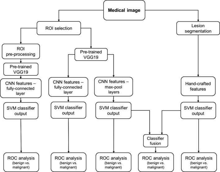
Lesion classification pipeline based on diagnostic images. Two types of features are extracted from a medical image: (a) CNN features with pretrained CNN and (b) handcrafted features with conventional CADx. High and low‐level features extracted by pretrained CNN are evaluated in terms of their classification performance and preprocessing requirements. Furthermore, the classifier outputs from the pooled CNN features and the handcrafted features are fused in the evaluation of a combination of the two types of features.

3. Deep neural network features

CNN features were extracted from the three datasets with the publicly available VGG19 model,¹¹ pretrained on ImageNet.¹² The CNN features were further used to train classifiers evaluated as described in Section 5. The architecture of the VGG19 model includes five stacks – with each stack containing two or four convolutional layers and a max‐pooling layer – followed by three fully connected layers. The VGG19 architecture and CNN feature‐extraction pipeline is illustrated in Fig. 2. VGG19 takes in an input to three RGB channels (Fig. 3). For the FFDM and ultrasound datasets, the ROIs were simply duplicated across the three channels since they were grayscale. For the DCE‐MRI dataset, ROIs extracted at the precontrast (t0) and first (t1) and second (t2) postcontrast DCE time‐points were input to the three channels.

Figure 2.

Architecture of VGG19 model. It takes in an image ROI as an input. The model comprises five blocks, each of which contains two or four convolutional layers and a max‐pooling layer. The five blocks are followed by three fully connected layers. Features are extracted from the five max‐pooling layers, average‐pooled across the channel (third) dimension, and normalized with L2 norm. The normalized features are concatenated to form the CNN feature vector. [Color figure can be viewed at wileyonlinelibrary.com]

Figure 3.

(a) Examples of DCE‐MRI transverse center slices with the corresponding ROIs extracted. On the left is a benign case and on the right is a malignant case. (b) ROIs, extracted from the precontrast time‐point (t0) and the first two postcontrast time‐points (t1, t2), input into the three color channels of VGG19. [Color figure can be viewed at wileyonlinelibrary.com]

3.A. Pooled features

CNN features were extracted from each of five max‐pool layers. Using a method similar to the one proposed by Zheng et al.,¹³ they were then average‐pooled¹⁴ along spatial dimensions, resulting in five feature vectors. Each of the five vectors were individually normalized with the Euclidean norm¹⁵ and concatenated to form a final CNN feature vector, which was then normalized again.

It should be noted that the DCE‐MRI and ultrasound datasets contained image ROIs of varying sizes. Typically, when extracting features from images of varying sizes, some form of preprocessing or resizing is necessary in order to ensure the extracted features correspond to the same spatial information across all images. However, by average pooling across the layers, the dimensionality of the features is reduced while preserving the spatial structure of the extracted feature maps. Pooling thus removes the need for preprocessing by producing feature vectors of identical length regardless of original input dimensions. Consequently, the original ROIs of varying sizes were directly input into VGG19 without any preprocessing.

3.B. Fully connected features

For comparison, CNN features were also extracted from the first fully connected layer. Due to the sparsity of fully connected features, all zero‐variance features were removed prior to analysis. Since the ultrasound and DCE‐MRI datasets had images of varying sizes, the effects of preprocessing were investigated to determine if fully connected features required resized input ROIs. First, fully connected features were extracted from the ROIs of original sizes with no preprocessing performed. Then for comparison, ROIs were preprocessed to have constant size prior to feature extraction. To form constant‐size ROIs, DCE‐MRI ROIs were enclosed in a frame with pixel values set to the average value of the surrounded ROI. Mirror‐padding was utilized to preprocess ultrasound ROIs to achieve the same input ROI sizes.

4. Conventional CADx features

As another baseline comparison, handcrafted (i.e., conventional CADx) features were automatically extracted from each dataset and were further used to train classifiers and evaluated as described in Section 5. The following subsections describe the conventional CADx features for each imaging modality dataset.

4.A. Conventional CADx mammography features

For the conventional CADx method, the center of each lesion had already been manually indicated, after which each lesion was automatically segmented and handcrafted lesion features were computer‐extracted from the image data. The segmentation for FFDM was a multiple‐transition point, gray‐level, region‐growing technique extensively described by the works of Huo et al. and Li et al.^{8, 16} The resulting FFDM features described quantitative physical properties of the segmented lesion, such as size, shape, texture, and morphology.

4.B. Conventional CADx ultrasound features

Ultrasound lesions were segmented using automatic contour optimization based on the average radial derivative, as described by Horsch et al.¹⁷ Like the FFDM features, the ultrasound features described lesion properties such as size, shape, texture, and morphology. Further details of the image features and how they are obtained can be found in the literature of Giger et al.¹⁸ as well as other, more recent works.^{9, 10}

4.C. Conventional CADx DCE‐MRI features

Using radiologist‐indicated lesion locations, the DCE‐MRI lesions were automatically segmented using a fuzzy c‐means approach,¹⁹ followed by the computer extraction of 38 handcrafted features. These features were designed based on the biological phenotypes of a lesion and characterize lesions in terms of their size, shape, morphology, enhancement texture, kinetics, and kinetics variance.^{20, 21, 22, 23}

5. Classification and evaluation methods

A nonlinear support vector machine (SVM)²⁴ with Gaussian radial basis function (RBF) kernel was utilized for classification using the CNN features and conventional CADx features (Python Version 2.7.12, Python Software Foundation). We refer to the classifiers based on CNN features and conventional CADx features as CNN‐based classifiers and conventional CADx classifiers, respectively. The SVM was chosen over other classification methods due to its ability to handle sparse high‐dimensional data, which is an attribute of the CNN features. SVM hyperparameters were optimized by an internal grid search with five‐fold cross‐validation.

The performances of the classifiers were evaluated by patient using receiver operating characteristic (ROC) analysis.^{25, 26} Area under the ROC curve (AUC), a metric that is independent of cancer prevalence, served as the figure of merit and was evaluated with five‐fold cross‐validation. Within the cross‐validation, training folds were standardized to zero mean and unit variance. The test folds were standardized with the statistics of the corresponding training folds.

In addition to performance evaluation of CNN‐based and conventional CADx classifiers, we assessed the performance of fusion classifiers that integrated both CNN‐based classifier outputs and conventional CADx classifier outputs. For this task, the outputs were fused by averaging them together.

Diagnostic discrimination performance of the CNN‐based and conventional CADx classifiers was compared to their performance in combination. In order to assess statistical significance, DeLong tests were performed.²⁷ Bonferroni‐Holm corrections were used to account for multiple comparisons.²⁸

6. Results

6.A. Pooled features vs. fully connected features

Within the CNN‐based methods, the classification performance of pooled features extracted from the original size ROIs was moderately stronger than that of fully connected features extracted from preprocessed ROIs (Table 2, Fig. 4). Fully connected features extracted from the original ROIs with varying sizes resulted in much poorer classification performance. This is likely because the fully connected features do not map to the same spatial location in the ROIs of varying sizes. Figure 4 shows the ROC curves for the CNN‐based classifiers.

Table 2.

Classification performance of CNN features obtained from five max‐pooling layers and from the first fully connected layer. Classification performance is assessed by ROC analysis in terms of AUC values

	Fully connected features (no preprocessing)	Fully connected features (with preprocessing)	Max‐pool features
FFDM	0.78 (se = 0.01)	N/A	0.81 (se = 0.01)
Ultrasound	0.77 (se = 0.01)	0.85 (se = 0.01)	0.87 (se = 0.01)
DCE‐MRI	0.79	0.82	0.87 (se = 0.01)

Figure 4.

Fitted binormal ROC curves comparing the predictive performance of different CNN‐based classifiers. Note that since FFDM ROIs were presented in uniform dimensions, there was no preprocessing done for that dataset. [Color figure can be viewed at wileyonlinelibrary.com]

6.B. Fusion of CNN‐based classifiers and conventional CADx classifiers

Since the CNN‐based classifiers trained on pooled features performed the best in malignancy assessment, they were chosen as the final CNN‐based classifiers to be fused with the conventional CADx classifiers. Fusion of the two types of classifiers outperformed any single type of classifier in the task of distinguishing benign and malignant lesions for each dataset. Figures 5 and 6 demonstrate the classification performances of CNN‐based and conventional CADx classifiers individually and in combination. Figures 7 and 8 show the classifier agreement levels for the two individual types of classifiers, as well as the potential decision boundaries for the fusion classifiers. Notably, there appears to be moderate disagreement between the CNN‐based classifiers and the CADx‐based classifiers across all imaging modalities, likely explaining why fusion improves predictive performance.

Figure 5.

AUC values for the benign vs. malignant lesion discrimination tasks for the CNN‐based, CADx‐bases, and fusion classifiers. P‐values were corrected for multiple comparisons with Bonferroni‐Holm corrections.

Figure 6.

Fitted binormal ROC curves comparing the performances of CNN‐based classifiers, CADx‐based classifiers, and fusion classifiers. The solid line represents the fusion classifier. The dotted line represents the CNN‐based classifier using pooled features. The dashed line represents the conventional CADx classifier using handcrafted features. [Color figure can be viewed at wileyonlinelibrary.com]

Figure 7.

Bland‐Altman plots for each of the imaging modalities. The figures illustrate classifier agreement between the CNN‐based classifier and the CADx‐based classifier. The y‐axis shows the difference between the SVM outputs of the two classifiers; the x‐axis shows the averaged output of the two classifiers. Since the averaged output is also the output of the fusion classifier, these plots also help visualize potential decision boundaries between benign and malignant classifications. [Color figure can be viewed at wileyonlinelibrary.com]

Figure 8.

A diagonal classifier agreement plot between the CNN‐based classifier and the conventional CADx classifier for FFDM. The x‐axis denotes the output from the CNN‐based classifier, and the y‐axis denotes the output from the conventional CADx classifier. Each point represents an ROI for which predictions were made. Points near or along the diagonal from bottom left to top right indicate high classifier agreement; points far from the diagonal indicate low agreement. ROI pictures of extreme examples of agreement/disagreement are included. [Color figure can be viewed at wileyonlinelibrary.com]

7. Discussion

We have shown that classifiers trained on deep features and existing conventional CADx features can be fused to significantly improve predictive performance in the task of breast lesion diagnosis across three separate imaging modalities. Furthermore, we demonstrated that our multilayer feature extraction methodology outperforms the commonly used approaches to deep feature extraction in addition to not requiring image preprocessing. We found that when extracting fully connected deep features from images, different ad hoc preprocessing techniques were required to maximize performance: ultrasound images worked best with mirror padding, but DCE‐MR images worked best with average pixel padding. By circumventing the need to resize images, our methodology is more generalizable across different datasets, while also commanding stronger predictive performance, less sparsity, and lower dimensionality.

We believe that this is the first development of a hybrid technique involving hierarchical deep feature extraction and conventional CADx methods. A previous paper from our laboratory⁷ investigated the feasibility of using pretrained CNNs and how they compare with conventional CADx methods, but only on a FFDM dataset. The FFDM dataset used for this study was larger with 26 extra lesions and 132 extra ROIs. These ROIs had been removed prior to analysis in our previous paper due to visual artifacts occluding areas of the lesion. We chose to include them for this study to see how CNN methods would handle cases with such artifacts. Additionally, we used a novel method of feature extraction inspired by the work of Zheng et al.,¹³ involving average pooling of extracted features from multiple CNN layers in order to considerably reduce dimensionality while preserving spatial structure and occlusion invariance. Our method avoided using higher‐level layers as Zheng et al. did, since higher‐level layers are more specific to the original ImageNet task of general object recognition. For CADx and medical images, lower‐level layers appear to be of greater importance, and our moderately sized datasets restricted us from freely including extra layers and parameters. Numerous other papers have used CNNs for computer‐aided diagnosis with success,^{6, 7, 29, 30, 31} but did not provide baseline comparisons with conventional CADx methods.

It is important to note that we used CNNs as fixed feature extractors instead of training them from scratch or fine‐tuning them.⁴ Our motivation for doing so is threefold: (a) Computational time: Using an NVIDIA GeForce GTX 970, feature extraction for our ultrasound dataset of 2393 images took approximately 3 min; fine‐tuning a CNN on the dataset takes between 8 and 24 h of training time. In an applied setting, models need to be retrained upon receiving new data, so the training time is nontrivial. (b) Validation: Our preliminary results involving fine‐tuning underperformed our feature extraction methods, but we are aware that fine‐tuning can often outperform generic feature extraction given the proper circumstances (e.g., ad hoc optimizations of hyperparameters/architectures, augmentation techniques, sufficient sample sizes). However, the slow training time of fine‐tuning limits the efficiency of data usage: standard validation procedures when training CNNs typically only separate the data into a single training set and a single test set. With feature extraction, we are able to use more rigorous validation procedures like k‐fold cross‐validation or bootstrapping, resulting in a more precise and reliable model. (c) Generalizability: Medical images vary dramatically based on institution and manufacturer. Consequently, it is important to have a method that quickly generalizes across these differences without overfitting to trivial nuances unique to single institutions or manufacturers. Our method only uses generic CNN features and radiomic features, eliminating the need to retrain a new CNN and use ad hoc hyperparameter optimizations for every new dataset.

Shin et al.³¹ reported that fine‐tuning substantially outperformed feature extraction in the task of computer‐aided detection, but they only extracted features from the final layer of AlexNet. Other works have shown that the final layer of AlexNet is significantly inferior to earlier layers for the task of medical image analysis.^{6, 7} Our method employs a more advanced feature extraction technique by hierarchically integrating multiple layers from VGGNet in order to incorporate both low‐ and high‐level information from images. It therefore remains unclear how fine‐tuning and feature extraction perform in comparison with each other.

There were several limitations to our study. While we used VGGNet, other networks, such as deep residual networks,³² have shown greater performances and promise for transfer learning, but their depth (upwards of 1000 layers) and complexity makes investigating their potential for CADx out of the scope of this study, especially due to the moderate sizes of our datasets. Furthermore, our datasets all came from one medical center. Due to the heterogeneity resulting from different imaging manufacturers and facility protocols, it is unknown whether our classifiers would test well on images from another institution. Additionally, the selection of contrast time‐points for the DCE‐MRI was suboptimal. In some of our preliminary experiments, we found that other combinations of contrast‐timepoints may perform better than the one we chose (t0, t1, and t2), warranting further investigation.

We also note that within our study, we reported cross‐validation performance scores instead of prediction scores on a held‐out test set. Although a typical model tuning procedure would involve a training set, validation set, and held‐out test set (two splits), we chose only to use a training set and a test set (one split) since we performed no prior feature selection or parameter optimization. Hyperparameter optimization was used for our SVMs during cross‐validation, but hyperparameter selections were held constant for each cross‐validation fold when reporting scores. Furthermore, using cross‐validation as the reported evaluation technique allowed us to more efficiently use the data – instead of reporting on one test set, we report on a score averaged across five test sets. Given a larger dataset, a standard training/validation/test split of the data would have been optimal, but cross‐validation on a single split seemed to be the better choice in terms of providing precise, robust model estimates given our smaller datasets and lack of parameter optimization.

In summary, we demonstrated the feasibility of using deep feature extraction techniques in CADx across three breast imaging modalities – mammography, ultrasound, and DCE‐MRI. Moreover, we developed a system incorporating both deep learning and conventional CADx methods that performed statistically significantly better than either one separately. Our methodology is computationally efficient, provides precise error estimates, and does not require intensive image preprocessing. Given the rapid progress of deep learning, our intent is not that our exact methodology be incorporated in clinical practices, but that our proposed solutions to the challenges of efficiency, precision, and preprocessing help pave the way toward more effective CADx methods.

References

- 1. Giger ML, Karssemeijer N, Schnabel JA. Breast image analysis for risk assessment, detection, diagnosis, and treatment of cancer. Annu Rev Biomed Eng. 2013;15:327–357. [DOI] [PubMed] [Google Scholar]
- 2. Zhang W, Doi K, Giger ML, Wu Y, Nishikawa RM, Schmidt R. A Computerized detection of clustered microcalcifications in digital mammograms using a shift‐invariant artificial neural network. Med Phys. 1994;21:517–524. [DOI] [PubMed] [Google Scholar]
- 3. Lo SCB, Chan HP, Lin JS, Li H, Freedman MT, Mun SK. Artificial convolution neural network for medical image pattern recognition. Neural Netw. 1995;8:1201–1214. [Google Scholar]
- 4. Yosinski J, Clune J, Bengio Y, Lipson H. How transferable are features in deep neural networks? Adv Neural Inf Process Syst. 2014;27:3320–3328. [Google Scholar]
- 5. Donahue J, Jia Y, Vinyals O, et al. DeCAF: A Deep Convolutional Activation Feature for Generic Visual Recognition. in Proceedings of The 31st International Conference on Machine Learning 647–655; 2014.
- 6. Bar Y, Diamant I, Wolf L, Greenspan H. Deep learning with non‐medical training used for chest pathology identification. in SPIE Medical Imaging 94140V–94140V–7 (International Society for Optics and Photonics; 2015).
- 7. Huynh BQ, Li H, Giger ML. Digital mammographic tumor classification using transfer learning from deep convolutional neural networks. J Med Imaging (Bellingham). 2016;3:034501. [DOI] [PMC free article] [PubMed] [Google Scholar]
- 8. Li H, Giger ML, Yuan Y, et al. Evaluation of computer‐aided diagnosis on a large clinical full‐field digital mammographic dataset. Acad Radiol. 2008;15:1437–1445. [DOI] [PMC free article] [PubMed] [Google Scholar]
- 9. Drukker K, Sennett CA, Giger ML. Automated method for improving system performance of computer‐aided diagnosis in breast ultrasound. IEEE Trans Med Imaging. 2009;28:122–128. [DOI] [PubMed] [Google Scholar]
- 10. Jamieson AR, Giger ML, Drukker K, Li H, Yuan Y, Bhooshan N. Exploring nonlinear feature space dimension reduction and data representation in breast CADx with Laplacian eigenmaps and t‐SNE. Med Phys. 2010;37:339–351. [DOI] [PMC free article] [PubMed] [Google Scholar]
- 11. Simonyan K, Zisserman A. Very Deep Convolutional Networks for Large‐Scale Image Recognition. arXiv [cs.CV]; 2014.
- 12. Deng J, Dong W, Socher R, Li LJ, Li K, Fei‐Fei L. ImageNet: A large‐scale hierarchical image database. in 2009 IEEE Conference on Computer Vision and Pattern Recognition; 2009. 10.1109/cvprw.2009.5206848. [DOI]
- 13. Zheng L, Zhao Y, Wang S, Wang J, Tian Q. Good Practice in CNN Feature Transfer. arXiv [cs.CV]; 2016.
- 14. LeCun Y, Bottou L, Bengio Y. Gradient‐based learning applied to document recognition. Proceedings of the; 1998.
- 15. Deza MM, Deza E. In Encyclopedia of Distances. Berlin, Heidelberg: Springer; 2009: pp. 1–583. [Google Scholar]
- 16. Huo Z, Giger ML, Vyborny CJ, et al. Analysis of spiculation in the computerized classification of mammographic masses. Med Phys. 1995;22:1569–1579. [DOI] [PubMed] [Google Scholar]
- 17. Horsch K, Giger ML, Venta LA, Vyborny CJ. Computerized diagnosis of breast lesions on ultrasound. Med Phys. 2002;29:157–164. [DOI] [PubMed] [Google Scholar]
- 18. Giger ML, Al‐Hallaq H, Huo Z, et al. Computerized analysis of lesions in US images of the breast. Acad Radiol. 1999;6:665–674. [DOI] [PubMed] [Google Scholar]
- 19. Chen W, Giger ML, Bick U. A fuzzy c‐means (FCM)‐based approach for computerized segmentation of breast lesions in dynamic contrast‐enhanced MR images. Acad Radiol. 2006;13:63–72. [DOI] [PubMed] [Google Scholar]
- 20. Gilhuijs KGA, Giger ML, Bick U. Computerized analysis of breast lesions in three dimensions using dynamic magnetic‐resonance imaging. Med Phys. 1998;25:1647–1654. [DOI] [PubMed] [Google Scholar]
- 21. Gibbs P, Turnbull LW. Textural analysis of contrast‐enhanced MR images of the breast. Magn Reson Med. 2003;50:92–98. [DOI] [PubMed] [Google Scholar]
- 22. Chen W, Giger ML, Li H, Bick U, Newstead GM. Volumetric texture analysis of breast lesions on contrast‐enhanced magnetic resonance images. Magn Reson Med. 2007;58:562–571. [DOI] [PubMed] [Google Scholar]
- 23. Bhooshan N, Giger ML, Jansen SA, Li H, Lan L, Newstead GM. Cancerous breast lesions on dynamic contrast‐enhanced MR images: computerized characterization for image‐based prognostic markers. Radiology. 2010;254:680–690. [DOI] [PMC free article] [PubMed] [Google Scholar]
- 24. Shawe‐Taylor J, Sun S. A review of optimization methodologies in support vector machines. Neurocomputing. 2011;74:3609–3618. [Google Scholar]
- 25. Metz CE, Pan X. ‘Proper’ binormal ROC curves: theory and maximum‐likelihood estimation. J Math Psychol. 1999;43:1–33. [DOI] [PubMed] [Google Scholar]
- 26. Pan X, Metz CE. The ‘Proper’ binormal model: parametric receiver operating characteristic curve estimation with degenerate data. Acad Radiol. 1997;4:380–389. [DOI] [PubMed] [Google Scholar]
- 27. DeLong ER, DeLong DM, Clarke‐Pearson DL. Comparing the areas under two or more correlated receiver operating characteristic curves: a nonparametric approach. Biometrics. 1988;44:837–845. [PubMed] [Google Scholar]
- 28. Holm S. A simple sequentially rejective multiple test procedure. Scand Stat Theory Appl. 1979;6:65–70. [Google Scholar]
- 29. Greenspan H, van Ginneken B, Summers RM. Guest editorial deep learning in medical imaging: overview and future promise of an exciting new technique. IEEE Trans Med Imaging. 2016;35:1153–1159. [Google Scholar]
- 30. Tajbakhsh N, Shin JY, Gurudu SR, et al. Convolutional neural networks for medical image analysis: full training or fine tuning? IEEE Trans Med Imaging. 2016;35:1299–1312. [DOI] [PubMed] [Google Scholar]
- 31. Shin HC, Roth HR, Gao M, et al. Deep convolutional neural networks for computer‐aided detection: CNN architectures, dataset characteristics and transfer learning. IEEE Trans Med Imaging. 2016;35:1285–1298. [DOI] [PMC free article] [PubMed] [Google Scholar]
- 32. He K, Zhang X, Ren S, Sun J. Deep residual learning for image recognition. in Proceedings of the IEEE Conference on Computer Vision and Pattern Recognition 770–778; 2016.