A Subspace Approach to Spectral Quantification for MR Spectroscopic Imaging

Abstract

Objective

To provide a new approach to spectral quantification for magnetic resonance spectroscopic imaging (MRSI), incorporating both spatial and spectral priors.

Methods

A novel signal model is proposed, which represents the spectral distributions of each molecule as a subspace and the entire spectrum as a union-of-subspaces. Based on this model, the spectral quantification can be solved in two steps: a) subspace estimation based on the empirical distributions of the spectral parameters estimated using spectral priors, and b) parameter estimation for the union-of-subspaces model incorporating spatial priors.

Results

The proposed method has been evaluated using both simulated and experimental data, producing impressive results.

Conclusions

The proposed union-of-subspaces representation of spatiospectral functions provides an effective computational framework for solving the MRSI spectral quantification problem with spatiospectral constraints.

Significance

The proposed approach transforms how the MRSI spectral quantification problem is solved and enables efficient and effective use of spatiospectral priors to improve parameter estimation. The resulting algorithm is expected to be useful for a wide range of quantitative metabolic imaging studies using MRSI.

I. Introduction

Magnetic resonance spectroscopic imaging (MRSI) is a unique tool for non-invasive, label-free molecular imaging [1], and spectral quantification is a critical step in deriving quantitative molecular information from the measured MRSI data. However, obtaining accurate spectral estimates is rather challenging due to the low signal-to-noise ratio (SNR) of the measured data and nonlinearity of the underlying parameter estimation problem.

While many computational solutions have been proposed to address the spectral quantification problem, model-based methods using spectral priors in the form of spectral basis functions have become the most popular [2–4]. The spectral basis functions obtained from either quantum mechanical simulations [5, 6] or in vitro experiments provide much stronger spectral constraints than earlier linear prediction based methods [7, 8], thereby resulting in significantly improved spectral estimates. However, these methods process MRSI data for each spatial location independently, and the uncertainty of the resulting spectral estimates from noisy MRSI data are often too big to be practically useful. To address this problem, spatial priors in the form of smoothness constraints were introduced [9–11]. However, such a formulation requires the solution of a large-scale constrained nonlinear optimization problem, especially for high-resolution MRSI. In this paper, we introduce a new subspace framework characterized by the use of a union-of-subspaces model to represent the desired spatiospectral function. The use of this model is motivated by its success in our previous ultrahigh-resolution MRSI work [12]. But the proposed method takes one step further to represent individual molecules using their own subspaces and allow different spatial constraints for individual spectral components. This model enables efficient and effective use of both spectral and spatial priors to improve spectral quantification of high-resolution MRSI data. A preliminary version of this work was reported in [13].

II. Proposed Method

A. Subspace Spectral Model

The current spectral model represents the noiseless spectroscopic signal with L spectral (or molecular) components as

$$s(t)=\sum _{\ell =1}^L{c}_{\ell }{\varphi }_{\ell }(\mathit{\beta },t),$$ (1)

where the c_ℓ denotes molecular concentration for the ℓ^th molecule and ϕ_ℓ(β, t) is the corresponding spectral basis function. In MRSI, both c_ℓ and ϕ_ℓ(β, t) are spatially dependent and Eq. (1) can be written explicitly as

$$s(\mathit{x},t)=\sum _{\ell =1}^L{c}_{\ell }(\mathit{x}){\varphi }_{\ell }(\mathit{\beta }(\mathit{x}),t),$$ (2)

The functional form of ϕ_ℓ(β, t) can be obtained using quantum mechanical simulations or in vitro experiments, in which the spectral parameters β are used to accommodate spectral variations under specific experimental conditions. Determining β often entails solving a nonlinear optimization problem. The conventional approaches determine c_ℓ(x) and β(x) point-by-point for each spatial location and the resulting estimates often have large uncertainties especially for MRSI data of low SNR. Determining c_ℓ(x) and β(x) jointly for all the spatial locations incorporating spatial constraints can reduce the estimation uncertainty but leads to a challenging optimization problem [11]. In this paper, we propose to use a subspace model to represent ϕ_ℓ(β, t). More specifically, assuming that ϕ_ℓ(β, t) resides in the Q_ℓ-dimensional subspace spanned by ${\{b_{\ell ,q}(t)\}}_{q=1}^{Q_{\ell }}$, we can express ϕ_ℓ(β, t) as

$${\varphi }_{\ell }(\mathit{\beta },t)=\sum _{q=1}^{Q_{\ell }}{a}_{\ell ,q}{b}_{\ell ,q}(t).$$ (3)

The model in Eq. (3) is motivated by the fact that ϕ_ℓ(β, t), viewed as a family of functions, resides in a low-dimensional subspace when β varies over a small range as is often the case in practice. To demonstrate this property, we use the spectral basis functions of N-acetylaspartate (NAA), myo-inositol (mI) and glutamate (Glu) as examples. We generated the basis functions using quantum mechanical simulations with β consisting of the relaxation time constant T₂ and the overall frequency shift Δf. We further assume that T₂ of NAA, mI and Glu are uniformly distributed over [150, 350] ms, [100, 300] ms and [75, 275] ms respectively based on the literature values [14] while Δf is uniformly distributed over [−5, 5] Hz. The set of functions ${\{\varphi ({\mathit{\beta }}_m,t)\}}_{m=1}^M$ for M = 5000 with β_m chosen based on the specified distribution are highly linearly dependent for a particular molecule. To see this more clearly, we form the following Casorati matrix using ${\{\varphi ({\mathit{\beta }}_m,t)\}}_{m=1}^M$ for each molecule:

$$\mathbf{C}=\left[\begin{array}{cccc}\hfill \varphi ({\mathit{\beta }}_1,t_1)\hfill & \hfill \varphi ({\mathit{\beta }}_1,t_2)\hfill & \hfill \dots \hfill & \hfill \varphi ({\mathit{\beta }}_1,t_n)\hfill \\ \hfill \varphi ({\mathit{\beta }}_2,t_1)\hfill & \hfill \varphi ({\mathit{\beta }}_2,t_2)\hfill & \hfill \dots \hfill & \hfill \varphi ({\mathit{\beta }}_2,t_n)\hfill \\ \hfill ⋮\hfill & \hfill ⋮\hfill & \hfill \ddots \hfill & \hfill ⋮\hfill \\ \hfill \varphi ({\mathit{\beta }}_M,t_1)\hfill & \hfill \varphi ({\mathit{\beta }}_M,t_2)\hfill & \hfill \dots \hfill & \hfill \varphi ({\mathit{\beta }}_M,t_n)\hfill \end{array}\right].$$ (4)

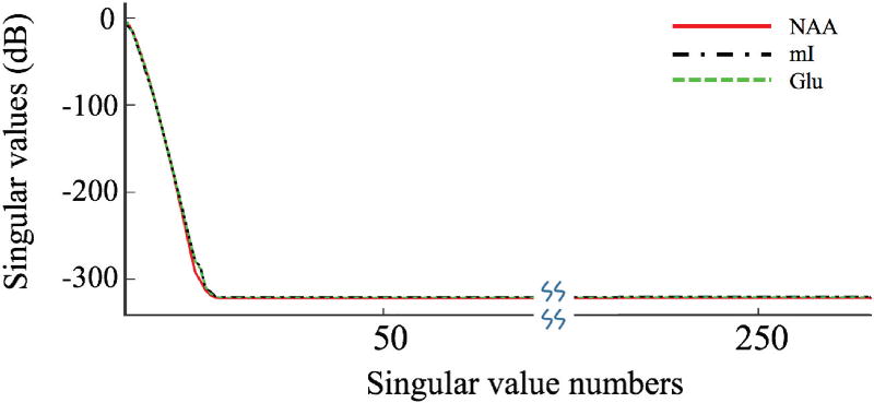
As can bee seen in Fig. 1, the Casorati matrices have rapidly decaying singular values for all three metabolites (rank < 16 in contrast to M = 5000).

Fig. 1.

Singular value distributions of the Casorati matrices defined in Eq. (4) for the spectral functions of NAA, mI and Glu respectively. Note that the singular values decay rapidly, signifying the low-rank nature of C. Equivalently, ${\{\varphi ({\mathit{\beta }}_m,t)\}}_{m=1}^M$ reside in a low-dimensional subspace.

Combining the low-dimensional representation for each molecule, we obtain a union-of-subspaces model for s(x, t) as

$$s(\mathit{x},t)=\sum _{\ell =1}^L\sum _{q=1}^{Q_{\ell }}{a}_{\ell ,q}(\mathit{x})b_{\ell ,q}(t),$$ (5)

where a_ℓ,q absorbs the c_ℓ in Eq. (1). This model converts a highly nonlinear model in Eq. (2) to a bilinear one, significantly simplifying the computational problem associated with joint spectral quantification with spatial constraints. This paper takes advantage of this important feature to improve spectral quantification from noisy MRSI data.

B. Subspace Estimation

Estimation of the subspace structure (i.e., ${\{b_{\ell ,q}(t)\}}_{q=1}^{Q_{\ell }}$) for each spectral component (or molecule) is an important step in the proposed method. To address this, we first estimate the distribution of β from the noisy measured data. This is done by solving the following nonlinear optimization problem point-by-point for all the voxels (p = 1, 2, …, P):

$$\{c_{p,\ell }^{\ast }\},{\mathit{\beta }}_p^{\ast }=\text{arg }\underset{\{c_{p,\ell }\},{\mathit{\beta }}_p}{\text{min}}\sum _{n=1}^N{\Vert d({\mathit{x}}_p,t_n)-\sum _{\ell =1}^L{c}_{p,\ell }{\varphi }_{\ell }({\mathit{\beta }}_p,t_n)\Vert }_2^2,$$ (6)

where t_n denotes the sampling time index and d(x_p, t_n) represents the measured data for s(x_p, t_n). This step is equivalent to what is done in conventional spectral quantification methods (e.g., QUEST [4]). However, instead of treating $\{c_{p,\ell }^{\ast }\}$ and ${\mathit{\beta }}_p^{\ast }$ as the final estimated spectral parameters as is done in the conventional methods, we use ${\{{\mathit{\beta }}_p^{\ast }\}}_{p=1}^P$ to create a Casorati matrix as defined in Eq. (4) (replacing M with P and ϕ with ϕ_ℓ). We then perform a singular value decomposition on the Casorati matrix and use the conjugate of its most dominant Q_ℓ right singular vectors as ${\{b_{\ell ,q}(t)\}}_{q=1}^{Q_{\ell }}$. In practice, Q_ℓ is selected such that the Q_ℓ+1th singular value decays below −50dB.

Note that for a large P as is the case in practice, ${\{{\mathit{\beta }}_p^{\ast }\}}_{p=1}^P$ define an empirical distribution P(β) for β. Then ${\{{\mathit{\beta }}_p^{\ast }\}}_{p=1}^P$ can be viewed as a set of sample values drawn from P(β). For a given P(β), different trials would give different sets of sample values but it can be justified that the Casorati matrices corresponding to different sets of sample values all share the “same” subspace. A detailed discussion of this issue is beyond the scope of this paper, and will be addressed in a future paper where the robustness of the proposed method for practical applications will be systematically analyzed. It is also worth noting that when the SNR of d(x_p, t) is low as is often the case, the ${\{{\mathit{\beta }}_p^{\ast }\}}_{p=1}^P$ as determined in Eq. (6) will lead to a biased distribution for P(β). To alleviate this problem, we determine ${\{{\mathit{\beta }}_p^{\ast }\}}_{p=1}^P$ at a lower spatial resolution to ensure good SNR for d(x_p, t_n) used in Eq. (6). This strategy is acceptable because we use ${\{{\mathit{\beta }}_p^{\ast }\}}_{p=1}^P$ only for subspace estimation not as the final spectral parameters, which is another desirable feature of the proposed method.

C. Spectral Quantification

Once the basis functions ${\{b_{\ell ,q}(t)\}}_{q=1}^{Q_{\ell }}$ are determined, we can fit the subspace model in Eq. (5) to the measured data to determine a_ℓ,q(x). We solve this problem for all the spatial locations (or voxels) jointly, incorporating any spatial priors available (e.g., spatial smoothness constraints). Incorporation of spatial priors about the spectral parameters has been demonstrated to be useful for improving spectral quantification [10, 11] but at the expense of significantly increased computational complexity. The proposed subspace model in Eq. (5) is a linear model, which makes it much easier to impose any spatial constraints on a_ℓ,q(x). To simplify notation, let a_ℓ,q = [a_ℓ,q(x₁), a_ℓ,q(x₂), …, a_ℓ,q(x_P)]^T denote the linear coefficients for a particular basis and $\mathit{a}={[{\mathit{a}}_{1,1}^T,{\mathit{a}}_{1,2}^T,\dots ,{\mathit{a}}_{1,Q_1}^T,\dots ,{\mathit{a}}_{L,1}^T,{\mathit{a}}_{L,2}^T,\dots ,{\mathit{a}}_{L,Q_L}^T]}^T$ denote the collection of all the coefficients. Following [10, 11], we formulate the problem as a regularization problem:

$${\mathit{a}}^{\ast }=\text{arg }\underset{\mathit{a}}{\text{min}}\sum _{p,n}{\Vert d({\mathit{x}}_p,t_n)-\sum _{\ell ,q}{a}_{\ell ,q}({\mathit{x}}_p)b_{\ell ,q}(t_n)\Vert }_2^2+R(\mathit{a}),$$ (7)

where R(·) represents a regularization functional imposing any desired spatial constraints. Two types of regularizations have been used for spectral quantification [10, 11]: a) weighted-L₂ regularization, and b) total variation regularization, both of which aim at imposing edge-preserving spatial smoothness on the linear coefficients. For weighted-L₂ regularization, R(·) can be expressed as

$$R(\mathit{a})=\sum _{\ell =1}^L{\lambda }_{\ell }\sum _{q=1}^{Q_{\ell }}{\Vert \mathbf{W}{\mathit{a}}_{\ell ,q}\Vert }_2^2,$$ (8)

where the λ_ℓ is a tunable regularization parameter and W is a weighting matrix derived from reference anatomical images [15]. For total variation regularization, R(·) is given by

$$R(\mathit{a})=\sum _{\ell =1}^L{\lambda }_{\ell }\sum _{q=1}^{Q_{\ell }}{\Vert \nabla {\mathit{a}}_{\ell ,q}\Vert }_1,$$ (9)

where ∇ denotes the gradient operator. In this paper, we use the weighted-L₂ regularization in Eq. (8) to demonstrate the power of the proposed subspace model. Extension to total variation regularization is relatively straightforward because the subspace model is linear. With weighted-L₂ regularization, the optimization problem in Eq. (7) can be solved by many algorithms such as conjugate gradient [16]. The regularization parameters can be selected using the discrepancy principle. The final concentration c_l(x) can be computed as $c_l(\mathit{x})={\sum }_{q=1}^{Q_l}{a}_{l,q}^{\ast }(\mathit{x})b_{l,q}(0)$.

III. Results And DISCUSSION

A. Simulation Study

The performance of the proposed method has been evaluated and compared to QUEST using a 2-D MRSI simulation data set synthesized using Eq. (1) with the spectral structures for different molecules generated from NMR-SCOPE [6]. The temporal sampling rate was set as 2000 Hz and the matrix size was 128 × 128. Common NMR detectable metabolites in the human brain were included, namely, N-acetylaspartate (NAA), creatine (Cr), choline (Cho), myo-inositol (mI), glutamate (Glu) and glutamine (Gln). The corresponding concentrations were designed to be smooth within each tissue (e.g., gray matter, white matter and cerebrospinal fluid) but different across tissue types.

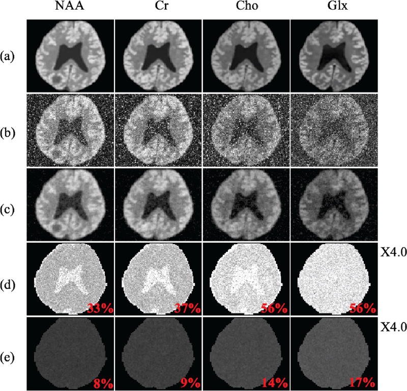
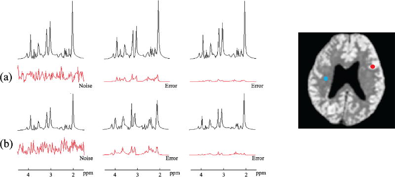
To validate the proposed method, we performed a Monte-Carlo study to compare the quantification results from the proposed method and QUEST. Figure 2 shows the estimation standard deviations from the Monte-Carlo study and the concentration maps estimated from one of the 40 realizations. Figure 3 shows a set of representative spectral fitting results including both the spectra synthesized using the estimated parameters and the error spectra compared to the ground truth. As can be seen, the spectral estimates obtained using the proposed method show significantly reduced errors and estimation variances.

Fig. 2.

Simulation results: (a) true concentration maps for NAA, Cr, Cho and Glx, (b) concentration maps estimated using QUEST, (c) concentration maps estimated using the proposed method, (d) standard deviation (SD) maps (normalized by the true concentrations) for QUEST, and (e) SD maps for the proposed method. The average SDs for each molecule are also shown (in red texts). Note the significant improvement in the estimated concentrations by the proposed method over QUEST.

Fig. 3.

Simulation results showing the quality of spectral estimation. Spectra from two representative locations marked by red and blue dots are shown in rows (a) and (b), respectively. The added noise in the original data and the estimation errors are shown in red. As can be seen, the proposed method produced more accurate spectral variations than QUEST.

B. In Vivo Study

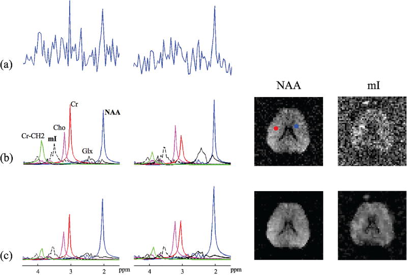
In vivo experiments were carried out to further evaluate the performance of the proposed method under practical conditions. One set of representative results is shown in Fig. 4, where the MRSI data were acquired from a healthy subject on a 3T MRI scanner using an echo-planar spectroscopic imaging (EPSI) sequence with outer-volume saturation [17] and water suppression [18]. The echo time was 30 ms, the echo spacing was 1.42 ms and the nominal in-plane resolution was 4.6 × 4.6 mm². The residual water and lipid signals were removed using the method proposed in [19]. The B₀ field inhomogeneity was corrected before quantification using the B₀ maps obtained from an auxiliary scan. It can be seen from Fig. 4 that the concentration maps produced by the proposed method show significantly reduced estimation variations than those from QUEST. These estimation results from the experimental data are consistent with those from the simulation study shown in Figs. 2 and 3.

Fig. 4.

Experimental results from an MRSI data set acquired using the conventional EPSI method: (a) noisy spectra from the voxels marked by the color dots, (b) quantification results from QUEST including the estimated individual spectral components and the concentration maps (the mI map is scaled by a factor of 3), and (c) quantification results from the proposed method.

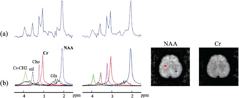
The proposed method has also been applied to processing a high-resolution MRSI data set acquired using the recently developed ultrafast MRSI technique known as SPICE [12]. The data set has a nominal in-plane resolution of 2.5 × 2.5 mm², and the estimation results from the proposed method are shown in Fig. 5. As can be seen, both the concentration maps and the spectral decomposition are of high quality, which is very encouraging especially for such a small voxel size.

Fig. 5.

Experimental results from a high-resolution MRSI data set produced by the SPICE technique: (a) two spectra from the voxels marked by the color dots, and (b) quantification results from the proposed method including the estimated individual spectral components and the concentration maps.

IV. CONCLUSION

This paper introduces a new approach to spectral quantification from noisy MRSI data using a subspace spectral model. This model represents the spectral distribution of each molecule using a subspace and the entire spectrum as a union-of-subspaces, which enables efficient incorporation of spectral and spatial priors to improve spectral quantification. The proposed approach has been evaluated using both simulated and experimental data, producing impressive results. The resulting algorithm is expected to be useful for a wide range of quantitative metabolic imaging studies using MRSI.

References

- 1.Posse S, et al. MR spectroscopic imaging: principles and recent advances. J Magn. Reson. 2013;37(6):1301–1325. doi: 10.1002/jmri.23945. [DOI] [PMC free article] [PubMed] [Google Scholar]
- 2.Provencher SW. Estimation of metabolite concentrations from localized in vivo proton NMR spectra. Magn. Reson. Med. 1993;30(6):672–679. doi: 10.1002/mrm.1910300604. [DOI] [PubMed] [Google Scholar]
- 3.Vanhamme L, et al. Improved method for accurate and efficient quantification of MRS data with use of prior knowledge. J Magn. Reson. 1997;129(1):35–43. doi: 10.1006/jmre.1997.1244. [DOI] [PubMed] [Google Scholar]
- 4.Ratiney H, et al. Time-domain semi-parametric estimation based on a metabolite basis set. NMR Biomed. 2005;18(1):1–13. doi: 10.1002/nbm.895. [DOI] [PubMed] [Google Scholar]
- 5.Soher BJ, et al. GAVA: spectral simulation for in vivo MRS applications. J Magn. Reson. 2007;185(2):291–299. doi: 10.1016/j.jmr.2007.01.005. [DOI] [PMC free article] [PubMed] [Google Scholar]
- 6.Stefan D, et al. Quantitation of magnetic resonance spectroscopy signals: the jMRUI software package. Meas. Sci. Technol. 2009;20(10):104035. [Google Scholar]
- 7.Barkhuijsen H, et al. Improved algorithm for noniterative time-domain model fitting to exponentially damped magnetic resonance signals. J Magn. Reson. 1987;73(3):553–557. [Google Scholar]
- 8.Barkhuijsen H, et al. Retrieval of frequencies, amplitudes, damping factors, and phases from time-domain signals using a linear least-squares procedure. J Magn. Reson. 1985;61(3):465–481. [Google Scholar]
- 9.Sava C, et al. Exploiting spatial information to estimate metabolite levels in two-dimensional MRSI of heterogeneous brain lesions. NMR Biomed. 2011;24(7):824–835. doi: 10.1002/nbm.1628. [DOI] [PubMed] [Google Scholar]
- 10.Kelm BM, et al. Using spatial prior knowledge in the spectral fitting of MRS images. NMR Biomed. 2012;25(1):1–13. doi: 10.1002/nbm.1704. [DOI] [PubMed] [Google Scholar]
- 11.Ning Q, et al. Spectral quantification for high-resolution MR spectroscopic imaging with spatiospectral constraints. IEEE Trans. Biomed. Eng. 2017;64(5):1178–1186. doi: 10.1109/TBME.2016.2594583. [DOI] [PMC free article] [PubMed] [Google Scholar]
- 12.Lam F, et al. High-resolution 1H-MRSI of the brain using spice: Data acquisition and image reconstruction. Magn. Reson. Med. 2015 doi: 10.1002/mrm.26019. [DOI] [PMC free article] [PubMed] [Google Scholar]
- 13.Li Y, et al. A subspace approach to spectral quantification. In Proc. Int. Soc. Magn. Reson. Med., Honolulu, HI, USA. 2017:871. [Google Scholar]
- 14.Träber F, et al. 1H metabolite relaxation times at 3.0 tesla: Measurements of T1 and T2 values in normal brain and determination of regional differences in transverse relaxation. J Magn. Reson. 2004;19(5):537–545. doi: 10.1002/jmri.20053. [DOI] [PubMed] [Google Scholar]
- 15.Haldar JP, et al. Anatomically constrained reconstruction from noisy data. Magn. Reson. Med. 2008;59(4):810–818. doi: 10.1002/mrm.21536. [DOI] [PubMed] [Google Scholar]
- 16.Eisenstat SC. Efficient implementation of a class of preconditioned conjugate gradient methods. SIAM J. Sci. Stat. Comp. 1981;2(1):1–4. [Google Scholar]
- 17.Le Roux P, et al. Optimized outer volume suppression for single-shot fast spin-echo cardiac imaging. J Magn. Reson. 1998;8(5):1022–1032. doi: 10.1002/jmri.1880080505. [DOI] [PubMed] [Google Scholar]
- 18.Haase A, et al. 1H NMR chemical shift selective (CHESS) imaging. Phys. Med. Biol. 1985;30(4):341. doi: 10.1088/0031-9155/30/4/008. [DOI] [PubMed] [Google Scholar]
- 19.Ma C, et al. Removal of nuisance signals from limited and sparse 1H MRSI data using a union-of-subspaces model. Magn. Reson. Med. 2016;75(2):488–497. doi: 10.1002/mrm.25635. [DOI] [PMC free article] [PubMed] [Google Scholar]