SEGMENTATION OF ORGANS AT RISK IN THORACIC CT IMAGES USING A SHARPMASK ARCHITECTURE AND CONDITIONAL RANDOM FIELDS

Abstract

Cancer is one of the leading causes of death worldwide. Radiotherapy is a standard treatment for this condition and the first step of the radiotherapy process is to identify the target volumes to be targeted and the healthy organs at risk (OAR) to be protected. Unlike previous methods for automatic segmentation of OAR that typically use local information and individually segment each OAR, in this paper, we propose a deep learning framework for the joint segmentation of OAR in CT images of the thorax, specifically the heart, esophagus, trachea and the aorta. Making use of Fully Convolutional Networks (FCN), we present several extensions that improve the performance, including a new architecture that allows to use low level features with high level information, effectively combining local and global information for improving the localization accuracy. Finally, by using Conditional Random Fields (specifically the CRF as Recurrent Neural Network model), we are able to account for relationships between the organs to further improve the segmentation results. Experiments demonstrate competitive performance on a dataset of 30 CT scans.

1. INTRODUCTION

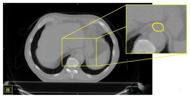
Cancer is one of the leading causes of death worldwide. Radiation therapy is an essential element of treatment for tumors such as in lung and esophageal cancer. Planning an irradiation begins with the delineation of the target tumor and healthy organs located near the target tumor, called Organs at Risk (OAR). Routinely, the delineation is largely manual which is tedious and source of anatomical errors. In the case of the esophagus, the shape and position vary greatly between patients, and its boundaries in CT images have low contrast and can be absent (Fig. 1).

Fig. 1.

CT scan with its manual delineation of the esophagus. Note how the esophagus is hardly distinguishable.

Several works have addressed the automatic segmentation of OAR problem, showing particular interest in the pelvic area [1, 2]. In [1] a framework is proposed for the segmentation of 17 organs at risk throughout the whole body, including brain, lungs, trachea, heart, liver, kidneys, prostate and rectum. The authors use 3 different techniques for different organs: thresholding, Generalized Hough Transform (GHT) and an atlas-registration based method. Another recent work was presented in [3] where the authors proposed to combine multi-atlas deformable registration with a level set-based local search to segment several organs, i.e., aorta, esophagus, trachea, heart. The results for the esophagus were not good enough for clinical usage with Dice ratio (DR) as low as 0.01; however, the results for the trachea were remarkably good with a DR between 0.82 and 0.95. For the heart and aorta, the mean DR values were around 0.80. These works rely heavily on preprocessing steps like edge preserving filtering for the case of GHT and registration results which can be very expensive computationally. More importantly, these works perform the segmentation of each organ individually, which ignores important information about the spatial relationships between them.

Recently, deep learning architectures have outperformed traditional methods and have achieved the state of the art in different imaging tasks like classification [4] and semantic segmentation, using the FCN [5]. Several extensions of the FCN [6, 7] have underlined that this architecture ignores the structured output required, producing very coarse results.

To overcome the mentioned difficulties, we propose to use a deep learning framework to address the joint segmentation of four thoracic organs at risk (esophagus, heart, trachea and aorta, in Fig. 2) with the assumption that, since these are neighboring organs, they can provide complementary information that can help the architecture to learn spatial relationships for boosting the performance. Specifically we use the SharpMask architecture inspired by the refinement frame-work presented in [8]. We experimentally show the superiority of this architecture in comparison with regular one path FCN. This is due to the ability of the network to combine low level features (from early layers) with high level features (from deep layers), reducing some of the issues that arise due to loss of resolution given by the use of pooling layers in semantic segmentation. Additionally, with the aim of overcoming the implicit coarseness given by FCN architecture, and to further enforce spatial relationships between the organs, we used Conditional Random Fields (CRF) as refinement step where different from other works [9], we used the CRFas- RNN [7] architecture since it allows the operation to be part of the network making the full system trainable end to end. Extensive experiments demonstrated that our method outperforms regular FCN architectures, their combination with CRF, and atlas methods like patch-based label fusion. We believe that the presented work is a step towards automated delineation in thoracic CT images, establishing a baseline system in joint thoracic OAR segmentation.

Fig. 2.

Typical CT scan with manual segmentation. Green represents the esophagus, yellow the heart, brown the trachea and blue the aorta.

2. METHOD

2.1. FCN and SharpMask feature fusion architecture

We use an FCN architecture with 10 layers where the first five are composed by convolutions, ReLU and max pooling operations. The last five layers are composed by transposed convolutions with ReLU operations and we use a voxel wise cross entropy loss. Note that the last layer contains 5 channels representing the probability maps for each organ plus background. This architecture is similar to the one presented in [10], but we do not use unpooling operations.

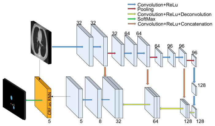
On the other hand, several works have shown that while in classification tasks deep networks that use pooling operations can have good results, the performance in semantic segmentation tasks can be affected due to loss of resolution. A common strategy is to use features from early layers along with high level features from deep layers, which has two big advantages: first it can improve the localization accuracy in the segmentation task, and second, it can help to alleviate the vanishing gradient problem since the errors from deep layers will be inserted in early layers. This has been exploited in the original FCN work [5], the U-Net [11], and more recently in SharpMask’s (SM) Facebook work [8]. In our work we used a SM architecture (Fig. 3) with the difference that instead of using bilinear upsampling in the refinement module, we used transposed convolutions which gives more parameters and hence more capacity to the network; additionally, we added a CRF module on top of the network which will be detailed in the next section. Different from [11], instead of copying the whole feature maps, convolution+ReLU operations are used to have the same number of channels as the deep level, avoiding the network to be biased due to big difference in the number of channels from early and deep layers.

Fig. 3.

Proposed architecture for multi-organ segmentation. The numbers indicate the number of channels at each layer.

2.2. Conditional Random Fields as RNN

A commonly used refinement step in semantic segmentation tasks is the CRF which has been used on top of classifiers with the aim of improving the consistency of the labels in a structured fashion. In the case of deep learning architectures, the output is coarse, and fully connected CRF have proved to refine the segmentation results providing fine edge details while allowing very efficient implementations [6, 12]. To perform inference, a mean field approximation is used [12] which involves an iterative algorithm. Given the label assignment x, a pairwise Gibbs energy is used as in [6]:

$$E(\mathit{x})=\sum _i{\psi }_u(x_i)+\sum _{ij}{\psi }_p(x_i,x_j)$$ (1)

where ψ_u(x_i) is the unary term, and typically is assigned as –logP(x_i), that is, the negative log-likelihood at voxel i. The pairwise term ψ_p(x_i, x_j) = μ(x_i, x_j)κ(f_i, f_j) measures the cost of assigning labels x_i, x_j simultaneously to voxels i, j, and $\kappa ({\mathit{f}}_i,{\mathit{f}}_j)={\sum }_{m=1}^M{\omega }^m{\kappa }^m({\mathit{f}}_i,{\mathit{f}}_j)$. Function μ is a compatibility function and each κ^m(f_i, f_j) is a Gaussian kernel between two feature vectors. We adopt the contrast-sensitive two-kernel potentials, as is widely done, defined in terms of intensities I_i and I_j and positions p_i and p_j : $\kappa ({\mathit{f}}_i,{\mathit{f}}_j)={\omega }^1\mathit{exp}(-\frac{{\mid {\mathit{p}}_i-{\mathit{p}}_j\mid }^2}{2{\sigma }_{\alpha }^2}-\frac{{\mid I_i-I_j\mid }^2}{2{\sigma }_{\beta }^2})+{\omega }^2\mathit{exp}(-\frac{{\mid {\mathit{p}}_i-{\mathit{p}}_j\mid }^2}{2{\sigma }_{\theta }^2})$. Recently, the authors [7] presented an approximation for doing inference in CRF by using backpropagable operations, allowing it to be used as part of the network and trainable end to end. This approach is no longer a separated postprocessing step, but a layer that can even learn some of its parameters. The module is shown in Fig. 3 (in orange), and its detailed architecture is presented in Fig. 4, where U represents the unary term and is defined as the unnormalized output (log likelihood) of the FCN. The I represents the input image, and it is used in the bilateral filter operation. Last, the dotted line is a feedback loop, implemented as a Recurrent Neural Network (RNN), which allows to backpropagate the errors by the backpropagation through time (BPTT) algorithm. This architecture allows the network to learn the ω^m parameters and the compatibility function μ. Typically the Potts model is used [9]; however, it has the limitation of giving a fixed penalty to similar voxels with different label assignments. Learning the compatibility function gives the flexibility of penalizing differently the organ assignments to voxel pairs according to their appearance and position, effectively accounting for relationships between them [7].

Fig. 4.

CRF as RNN architecture

3. EXPERIMENTS

We perform experiments on the standard FCN architecture and its extension with CRF as baseline methods, and then compare the results with our proposed architecture. We use rather large kernel size (7×7), in accordance with other works in CT images [9]. Regarding the CRF refinement, the training must be done in two steps; first we train a model without the CRF module, and then we train a new system where we fine-tune the weights of the learned model including the CRF module. This is a necessary step because, as shown in Eq. (1) and Fig. 4, we need a unary term that represents an (unnormalized) probability distribution of the labels for performing approximate inference.

3.1. Dataset and pre-processing

We evaluate our method on a dataset of 30 thoracic CT scans where the patients have either lung cancer or Hodgkin lymphoma, along with the manual delineations of the esophagus, heart, trachea, aorta and body contour. The latter is used in the network to avoid using background information during training. Scans have a resolution of 0.98×0.98×2.5 for a size of 512×512× (150×284) voxels. As pre-processing, each scan is normalized to have zero mean and unit variance. We perform 6-fold cross validation, resulting in 25 subjects for training and 5 for testing. The dataset is augmented applying a random affine transform and a randomly deformed version of each scan by using a deformation field obtained through a 2×2×2 grid of control-points and B-spline interpolation [13].

3.2. Training

The classes are imbalanced, i.e., the number of voxels for one organ are very different from another. We thus use a weighted cross entropy loss function. Specifically, we propose to fine-tune the learned weights, using the regular cross entropy loss without class weighting. Stochastic gradient descent (SGD) is then used with a learning rate of 0.1 which was decreased by a factor of ten every 20 epochs and initialized by Xavier initialization [14] for all the weights in the networks.

3.3. Results

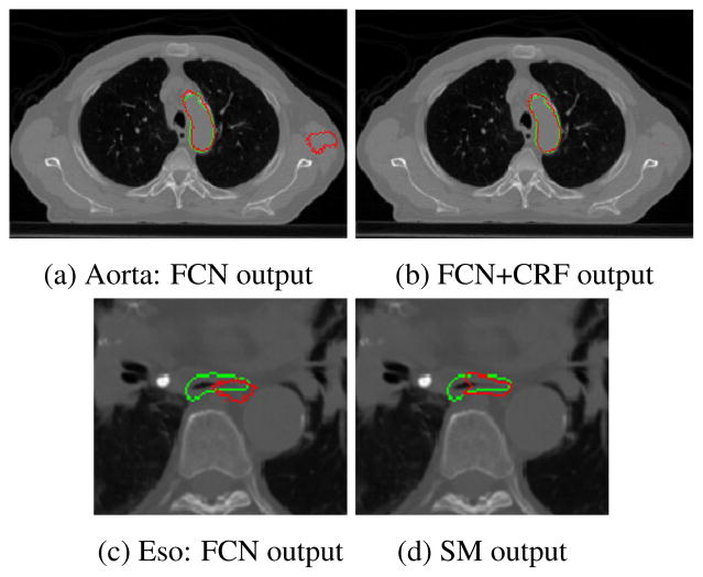
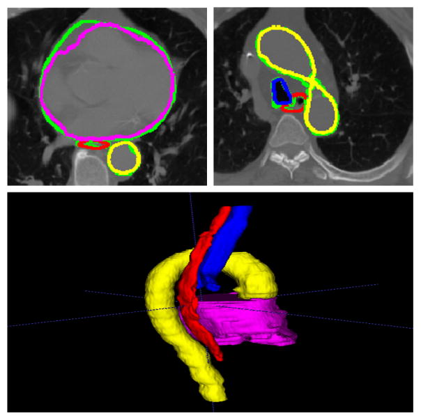
In Fig. 5 we show the segmentation result of the aorta and the esophagus for a slice of a testing CT scan. We can see that the FCN+CRF eliminated the false positive region on the right of the image. In the same figure, we show how the proposed architecture outperforms other methods in segmenting the esophagus, which is the most difficult organ. We can see that the localization is much better than that by the regular FCN. This is due to the fusion of high resolution features to alleviate the loss of precision due to pooling operations, which are still necessary to create highly semantic representations. Finally, in Fig. 6 we show the segmentation results for the four organs and their 3D rendering for one of the testing subjects.

Fig. 5.

Example of segmentation results in the aorta [a,b] (top) and esophagus [c,d] (bottom). Green is the ground truth and red the output of the system.

Fig. 6.

Segmentation results showing the four organs. The ground truth is green, and the output of the network is red for the esophagus, magenta for the heart, blue for the trachea and yellow for the aorta. The 3D rendering of the segmentation results is also shown on the bottom.

In Table 1 we present the DR obtained using each of the computer models, in addition to the results obtained by a patch based label fusion method called Optimized PatchMatch for Near Real Time and Accurate Label Fusion (OPAL) [15]. The most simple approach (OPAL) outperformed FCN-based architecture for the trachea. The trachea has a distinguishable dark intensity in CT images, and is surrounded by a lot of non-dark voxels; this makes an algorithm like OPAL work well since it will try to find similar patches in close areas. However, it requires images to be registered to a common space. This situation is different for organs with large intensity variation, and becomes even worse for the low contrast organs like the esophagus as can be seen from Table 1. Highest performance for each of the organs is obtained by SM-based architectures, and the difference with FCN is statistically significant (assessed by a paired t-test): p < 0.05 for all organs – except the aorta. Interestingly, the CRF refinement module is shown to be not that significant, when switching from one base architecture to a CRF based one, for both FCN and SM (as can be seen from the p-value for the latter case).

Table 1.

Comparison of mean DR ± stdev by different methods. First line of p-value: comparison to FCN; 2nd line: comparison to SM.

	OPAL	FCN	FCN+CRF	SM	SM+CRF
Eso.	0.39±0.05	0.60±0.04	0.57±0.06	0.66±0.08 p=0.13	0.67±0.04 p=0.01 p=0.79
Heart	0.62±0.07	0.86±0.03	0.87±0.02	0.89±0.02 p=0.07	0.90±0.01 p=0.01 p=0.30
Trachea	0.80±0.03	0.72±0.03	0.74±0.02	0.83±0.06 p=0.01	0.82±0.06 p=0.01 p=0.78
Aorta	0.49±0.10	0.83±0.06	0.81±0.08	0.85±0.06 p=0.58	0.86±0.05 p=0.37 p=0.76

4. CONCLUSIONS

We have presented a framework for joint segmentation of the esophagus, heart, trachea and aorta in CT images. The method uses data augmentation and a SharpMask architecture allowing an effective combination of low-level features with high-level semantic features. Additionally, the CRFasRNN enforces spatial relationships between organs improving the results. We are currently engaged in investigating new ways to incorporate context, such as in auto-context models.

References

- 1.Han M, et al. Segmentation of organs at risk in ct volumes of head, thorax, abdomen, and pelvis. Proc SPIE. 2015;9413:94133J–94133J–6. [Google Scholar]
- 2.Guinin M, et al. Segmentation of pelvic organs at risk using superpixels and graph diffusion in prostate radiotherapy. ISBI. 2015:1564–1567. [Google Scholar]
- 3.Schreibmann E, et al. Multiatlas segmentation of thoracic and abdominal anatomy with level set-based local search. J Appl Clin Med Phys. 2014;15(4) doi: 10.1120/jacmp.v15i4.4468. [DOI] [PMC free article] [PubMed] [Google Scholar]
- 4.Simonyan K, Zisserman A. Very deep convolutional networks for large-scale image recognition. CoRR. 2014;abs/1409.1556 [Google Scholar]
- 5.Long J, et al. Fully convolutional networks for semantic segmentation. CVPR. 2015 doi: 10.1109/TPAMI.2016.2572683. [DOI] [PubMed] [Google Scholar]
- 6.Chen L-C, et al. Semantic image segmentation with deep convolutional nets and fully connected crfs. ICLR. 2015 doi: 10.1109/TPAMI.2017.2699184. [DOI] [PubMed] [Google Scholar]
- 7.Zheng S, et al. Conditional random fields as recurrent neural networks. ICCV. 2015 [Google Scholar]
- 8.Pinheiro PHO, et al. Learning to refine object segments. CoRR. 2016;abs/1603.08695 [Google Scholar]
- 9.Dou Q, et al. 3d deeply supervised network for automatic liver segmentation from CT volumes. CoRR. 2016;abs/1607.00582 [Google Scholar]
- 10.Noh H, et al. Learning deconvolution network for semantic segmentation. ICCV. 2015 [Google Scholar]
- 11.Ronneberger O, et al. U-net: Convolutional networks for biomedical image segmentation. MICCAI. 2015;9351:234–241. [Google Scholar]
- 12.Kräahenbühl P, Koltun V. Efficient inference in fully connected crfs with gaussian edge potentials. NIPS. 2011 [Google Scholar]
- 13.Milletari F, et al. V-net: Fully convolutional neural networks for volumetric medical image segmentation. CoRR. 2016;abs/1606.04797 [Google Scholar]
- 14.Glorot X, Bengio Y. Understanding the difficulty of training deep feedforward neural networks. AISTATS. 2010 [Google Scholar]
- 15.Ta V-T, et al. Optimized patchmatch for near real time and accurate label fusion. MICCAI. 2014:105–112. doi: 10.1007/978-3-319-10443-0_14. [DOI] [PubMed] [Google Scholar]