Common pitfalls in statistical analysis: Measures of agreement

Abstract

Agreement between measurements refers to the degree of concordance between two (or more) sets of measurements. Statistical methods to test agreement are used to assess inter-rater variability or to decide whether one technique for measuring a variable can substitute another. In this article, we look at statistical measures of agreement for different types of data and discuss the differences between these and those for assessing correlation.

INTRODUCTION

Often, one is interested in knowing whether measurements made by two (sometimes more than two) different observers or by two different techniques produce similar results. This is referred to as agreement or concordance or reproducibility between measurements. Such analysis looks at pairs of measurements, either both categorical or both numeric, with each pair having been made on one individual (or a pathology slide, or an X-ray).

Superficially, these data may appear to be amenable to analysis using methods used for 2 × 2 tables (if the variable is categorical) or correlation (if numeric), which we have discussed previously in this series.[1,2] However, a closer look would show that this is not true. In those methods, the two measurements on each individual relate to different variables (e.g., exposure and outcome, or height and weight, etc), whereas in the “agreement” studies, the two measurements relate to the same variable (e.g., chest radiographs rated by two radiologists or hemoglobin measured by two methods).

WHAT IS AGREEMENT?

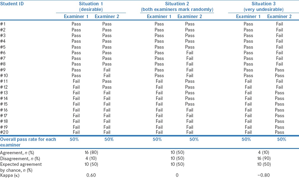
Let us consider the case of two examiners A and B evaluating answer sheets of 20 students in a class and marking each of them as “pass” or “fail,” with each examiner passing half the students. Table 1 shows three different situations that may happen. In situation 1 in this table, eight students receive a “pass” grade from both the examiners, eight receive a “fail” grade from both the examiners, and four receive pass grade from one examiner but “fail” grade from the other (two passed by A and the other two by B). Thus, the two examiners’ results agree for 16/20 students (agreement = 16/20 = 0.80, disagreement = 4/20 = 0.20). This seems quite good. However, this fails to take into account that some of the grades may have been guesswork and that the agreement may have occurred just by chance.

Table 1.

Results of 20 students, each evaluated independently by two examiners

Let us now consider a hypothetical situation where examiners do exactly this, i.e., assign grades by tossing a coin; heads = pass, tails = fail Table 1, Situation 2]. In that case, one would expect 25% (=0.50 × 0.50) of students to receive pass grade from both and another 25% to receive “fail” grade from both – an overall “expected” agreement rate for “pass” or “fail” of 50% (=0.25 + 0.25 = 0.50). Hence, the observed agreement rate (80% in situation 1) needs to be interpreted keeping in mind that 50% agreement was expected purely by chance. These examiners could have bettered this by 50% (best possible agreement minus the agreement expected by chance = 100%−50% =50%), but achieved only 30% (observed agreement minus the agreement expected by chance = 80%−50% =30%). Thus, their real performance in being concordant is 30%/50% = 60%.

Of course, they could theoretically have performed worse than what was expected by chance. For instance, in situation 3 [Table 1], even though each of them passed 50% of students, their grades agreed for only 4 of the 20 students – far fewer than that expected even by chance!

It is important to note that, in each of the three situations in Table 1, the pass percentages for the two examiners are equal, and if the two examiners are compared using a usual 2 × 2 test for paired data (McNemar's test), one would find no difference between their performances; by contrast, the inter-observer agreement in the three situations is widely different. The basic concept to be understood here is that “agreement” quantifies the concordance between the two examiners for each of the “pairs” of scores and not the similarity of the overall pass percentage between the examiners.

METHODS USED TO MEASURE AGREEMENT

The statistical methods used to assess agreement vary depending on the type of variable being studied and the number of observers between whom agreement is sought to be assessed. These are summarized in Table 2 and discussed below.

Table 2.

Methods used for assessment of agreement between observers depending on the type of variable measured and the number of observers

ASSESSING AGREEMENT BETWEEN MEASUREMENTS OF CATEGORICAL VARIABLES

Two observers assessing the same binary outcome (Cohen's kappa)

Cohen's kappa (κ) calculates inter-observer agreement taking into account the expected agreement by chance as follows:

κ = (observed agreement [P_o] – expected agreement [P_e])/(1-expected agreement [P_e]).

In the above example [Table 1, Situation 1], Cohen's k = (0.80 − 0.50)/(1 − 0.50) = 0.30/0.50 = 0.60.

The κ statistic can take values from − 1 to 1, and is interpreted somewhat arbitrarily as follows: 0 = agreement equivalent to chance; 0.10–0.20 = slight agreement; 0.21–0.40 = fair agreement; 0.41–0.60 = moderate agreement; 0.61–0.80 = substantial agreement; 0.81–0.99 = near-perfect agreement; and 1.00 = perfect agreement. Negative values indicate that the observed agreement is worse than what would be expected by chance. An alternative interpretation offered is that kappa values below 0.60 indicate a significant level of disagreement.

Cohen's κ can also be used when the same rater evaluates the same patients at two time points (say 2 weeks apart) or, in the example above, grades the same answer sheets again after 2 weeks. Its limitations are: (i) it does not take into account the magnitude of differences, making it unsuitable for ordinal data, (ii) it cannot be used if there are more than two raters, and (iii) it does not differentiate between agreement for positive and negative findings – which may be important in clinical situations (e.g., wrongly diagnosing a disease versus wrongly excluding it may have different consequences).

Variations of Cohen's κ

Weighted kappa

For ordinal data, where there are more than two categories, it is useful to know if the ratings by different raters varied by a small degree or by a large amount. For example, microbiologists may rate bacterial growth on culture plates as: none, occasional, moderate, or confluent. Here, ratings of a particular plate by two reviewers as “occasional” and “moderate,” respectively, would imply a lower level of discordance than if these ratings were “no growth” and “confluent,” respectively. The weighted Kappa statistic takes this difference into account. It thus yields a higher value when the raters’ responses correspond more closely, with the maximum scores for perfect agreement; conversely, a larger difference in two ratings provides a lower value of weighted kappa. Techniques for assigning weightage to the difference between categories (linear, quadratic) can vary.

Fleiss’ kappa

This method is used when ratings by more than two observers are available for either binary or ordinal data.

ASSESSING AGREEMENT BETWEEN MEASUREMENTS OF CONTINUOUS VARIABLES

Two methods are available for assessing agreement between measurements of a continuous variable across observers, instruments, time points, etc. One of these, namely intra-class correlation coefficient (ICC), provides a single measure of the extent of agreement, and the other, namely Bland–Altman plot, in addition, provides a quantitative estimate of how closely the values from two measurements lie.

Intra-class correlation coefficient

Let us think of two ophthalmologists measuring intraocular pressure using a tonometer. Each patient will thus have two readings – one by each observer. ICC provides an estimate of overall concordance between these readings. It is somewhat akin to “analysis of variance” in that it looks at the between-pair variances expressed as a proportion of the total variance of the observations (i.e., the total variability in “2n” observations, which would be expected to be the sum of within- and between-pair variances). The ICC can take a value from 0 to 1, with 0 indicating no agreement and 1 indicating perfect agreement.

Bland–Altman plots

When two instruments or techniques are used to measure the same variable on a continuous scale, the Bland–Altman plots can be used to estimate agreement. This plot is a scatter plot of the difference between the two measurements (Y-axis) against the average of the two measurements (X-axis). Thus, it provides a graphical display of bias (mean difference between the two observers or techniques) with 95% limits of agreement. The latter are given by the formula:

• Limits of agreement = mean observed difference ± 1.96 × standard deviation of observed differences.

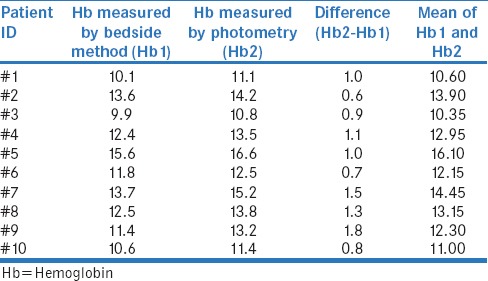
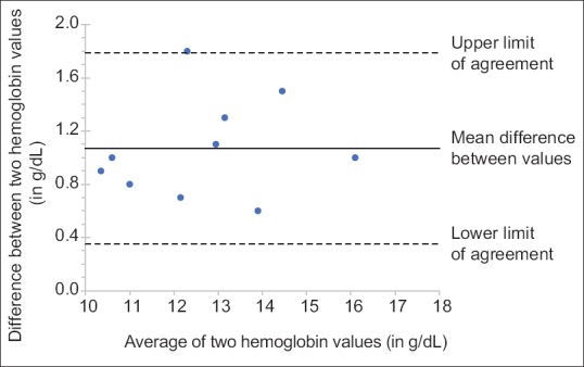
Consider a situation where we wish to assess the agreement between hemoglobin measurements (in g/dL) using a bedside hemoglobinometer and the formal photometric laboratory technique in ten persons [Table 3]. The Bland–Altman plot for these data shows the difference between the two methods for each person [Figure 1]. The mean difference between the values is 1.07 g/dL (with standard deviation of 0.36 g/dL), and the 95% limits of agreement are 0.35–1.79. What this implies is that hemoglobin level of a particular person measured by photometry could vary from that measured by the bedside method from as little as 0.35 g/dL higher to as much as 1.79 g/dL higher (this is the case for 95% of individuals; for 5% of individuals, variations could be outside these limits). This obviously means that the two techniques cannot be used as substitutes for one another. Importantly, there is no uniform criterion for what constitutes acceptable limits of agreement; this is a clinical decision and depends on the variable being measured.

Table 3.

Hemoglobin measurements in ten patients using two different methods

Figure 1.

Bland–Altman plot for data shown in Table 3. The upper and lower limits of agreement are generally drawn at 1.96 (roughly 2) standard deviations (of observed inter-observer differences) above and below the line representing the mean difference (solid line); these dotted lines are expected to enclose 95% of the observed inter-observer differences

POINTS TO REMEMBER

Correlation versus agreement

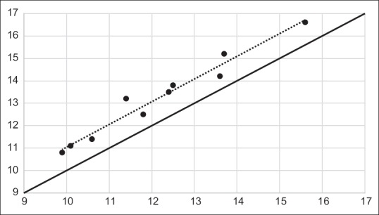
As alluded to above, correlation is not synonymous with agreement. Correlation refers to the presence of a relationship between two different variables, whereas agreement looks at the concordance between two measurements of one variable. Two sets of observations, which are highly correlated, may have poor agreement; however, if the two sets of values agree, they will surely be highly correlated. For instance, in the hemoglobin example, even though the agreement is poor, the correlation coefficient between values from the two methods is high [Figure 2]; (r = 0.98). The other way to look at it is that, though the individual dots are not fairly close to the dotted line (least square line;[2] indicating good correlation), these are quite far from the solid black line, which represents the line of perfect agreement (Figure 2: the solid black line). In case of good agreement, the dots would be expected to fall on or near this (the solid black) line.

Figure 2.

Scatter plot showing correlation between hemoglobin measurements from two methods for data shown in Table 3 and Figure 1. The dotted line is a trend line (least squares line) through the observed values, and the correlation coefficient is 0.98. However, the individual dots are far away from the line of perfect agreement (solid black line)

Use of paired tests to assess agreement

For all the three situations shown in Table 1, the use of McNemar's test (meant for comparing paired categorical data) would show no difference. However, this cannot be interpreted as an evidence of agreement. The McNemar's test compares overall proportions; therefore, any situation where the overall proportion of pass/fail by the two examiners is similar (e.g., situations 1, 2, and 3 in Table 1) would result in a lack of difference. Similarly, the paired t-test compares mean difference between two observations in a group. It can therefore be nonsignificant if the average difference between the paired values is small, even though the differences between two observers for individuals are large.

SUGGESTED READING

The readers are referred to the following papers that feature measures of agreement:

1. Qureshi et al. compared the grade of prostatic adenocarcinoma as assessed by seven pathologists using a standard system (Gleason's score).[3] Concordance between each pathologist and the original report and between pairs of pathologists was determined using Cohen's kappa. It is a useful example. However, we feel that, Gleason's score being an ordinal variable, weighted kappa might have been a more appropriate choice

2. Carlsson et al. looked at inter- and intra-observer variability in Hand Eczema Extent Score in patients with hand eczema.[4] Inter- and intra-observer reliability was assessed using the ICC

3. Kalantri et al. looked at the accuracy and reliability of pallor as a tool for detecting anemia.[5] They concluded that “Clinical assessment of pallor can rule out and modestly rule in severe anemia.” However, the inter-observer agreement for detecting pallor was very poor (kappa values = 0.07 for conjunctival pallor and 0.20 for tongue pallor) which means that pallor is an unreliable sign for diagnosing anemia.

Financial support and sponsorship

Nil.

Conflicts of interest

There are no conflicts of interest.

REFERENCES

- 1.Ranganathan P, Pramesh CS, Aggarwal R. Common pitfalls in statistical analysis: Logistic regression. Perspect Clin Res. 2017;8:148–51. doi: 10.4103/picr.PICR_87_17. [DOI] [PMC free article] [PubMed] [Google Scholar]
- 2.Aggarwal R, Ranganathan P. Common pitfalls in statistical analysis: The use of correlation techniques. Perspect Clin Res. 2016;7:187–90. doi: 10.4103/2229-3485.192046. [DOI] [PMC free article] [PubMed] [Google Scholar]
- 3.Qureshi A, Lakhtakia R, AL Bahri M, Al Haddabi I, Saparamadu A, Shalaby A, et al. Gleason's grading of prostatic adenocarcinoma: Inter-observer variation among seven pathologists at a tertiary care center in Oman. Asian Pac J Cancer Prev. 2016;17:4867–8. doi: 10.22034/APJCP.2016.17.11.4867. [DOI] [PMC free article] [PubMed] [Google Scholar]
- 4.Carlsson A, Svensson Š, Anderson CD, Baranovskaya I, Hindsén-Stenström M, Holt I, et al. Scoring of hand eczema: Good reliability of hand eczema extent score (HEES) Acta Derm Venereol. 2017;97:193–7. doi: 10.2340/00015555-2521. [DOI] [PubMed] [Google Scholar]
- 5.Kalantri A, Karambelkar M, Joshi R, Kalantri S, Jajoo U. Accuracy and reliability of pallor for detecting anaemia: A hospital-based diagnostic accuracy study. PLoS One. 2010;5:e8545. doi: 10.1371/journal.pone.0008545. [DOI] [PMC free article] [PubMed] [Google Scholar]