Automated Tracking of Cell Migration with Rapid Data Analysis

Abstract

Cell migration is essential for many biological processes including development, wound healing and metastasis. However, studying cell migration often requires the time-consuming and labor-intensive task of manually tracking cells. To accelerate the task of obtaining coordinate positions of migrating cells, we have developed a graphical user interface (GUI) capable of automating the tracking of fluorescently labeled nuclei. This GUI provides an intuitive user interface that makes automated tracking accessible to researchers with no image processing experience or familiarity with particle-tracking approaches. Using this GUI, users can interactively determine a minimum of four parameters to identify fluorescently labeled cells and automate acquisition of cell trajectories. Additional features allow for batch processing of numerous time-lapse images, curation of unwanted tracks, and subsequent statistical analysis of tracked cells. Statistical outputs allow users to evaluate migratory phenotypes, including cell speed, distance, displacement and persistence as well as measures of directional movement, such as forward migration index (FMI) and angular displacement.

Introduction

Cell migration is a fundamental biological process during development, wound healing and metastasis (Friedl and Alexander, 2011; Mayor and Theveneau, 2013; Singer and Clark, 1999). Neural crest cells migrate to distant regions of the embryo before undergoing differentiation. Fibroblasts infiltrate into wounded tissues, and keratinocytes migrate over a fibrin bed to repair a disrupted epidermal barrier, while cancer cells metastasize to distant tissues. Much of our understanding of these diverse processes has been obtained by studying cell migration in model systems that permit visualization of migratory behavior.

Increased access to microscopes capable of fluorescence and time-lapse imaging has made obtaining movies of migrating cells commonplace. Processing these movies typically requires manual annotation of cellular positions to then assemble cell trajectories and extract migratory information. However, this process is a time-intensive, rate-limiting step for migration experiments. While manual tracking of migrating cells has provided substantial insight into migratory processes in multiple fields of biology, new approaches have been adopted to accelerate this phase of migration research.

Particle-tracking applications have been repurposed to automate cell tracking and meet a pressing need of the cell biology community to accelerate acquisition of migration data (Masuzzo et al., 2016; Meijering et al., 2009). The most efficient of these automated approaches require fluorescent labeling of cells or nuclei. The high signal-to-noise ratio obtained with fluorescent labeling enables discrimination between particles of interest and non-specific noise. While some programs do enable tracking of phase-contrast images (Cordelieres et al., 2013; Hand et al., 2009; Piccinini et al., 2016), optimizing parameter settings can be challenging and the results can be quite variable. Many automated cell tracking options are open-source and therefore easily obtained, but becoming familiar with what each software can do and then choosing which to use can be daunting.

We provide a detailed protocol for a user friendly Graphical User Interface (GUI) capable of automating the acquisition of cell trajectories for the purpose of studying cell migration in low and high-density, 2-dimensional cell cultures. Intended users of the FastTracks GUI are novice and experienced cell biologists seeking to accelerate the acquisition of migratory data. No prior knowledge of image processing or particle tracking is necessary. All that is required is an 8-bit .tif movie of fluorescently labeled cells and a minimum of four interactive inputs to instantly obtain cell trajectories and migratory statistics from your experiment.

This unit guides you through the necessary steps to obtain the FastTracks automated tracking software and a detailed description of how to acquire and analyze migratory data using this program. Basic Protocol 1 describes the GUI and input parameters required to obtain positional coordinates for fluorescently labeled nuclei and subsequent generation of migratory tracks. Basic Protocol 2 describes features available to obtain statistics necessary for analysis of migratory behavior. Support Protocol 1 describes how to obtain MATLAB program files and a Windows executable to run FastTracks. Support Protocol 2 guides you through a feature for deleting specific tracks. Support Protocol 3 outlines how to process a batch of time-lapse movies once parameter settings have been optimized using Basic Protocol 1, and Support Protocol 4 describes how to mask regions of interest from time-lapse movies prior to tracking.

Basic Protocol 1 Obtaining Cell Tracks

The following instructions provide a quick overview of how to load time-lapse images, set parameters to identify cell nuclei, and acquire cell trajectories. Once a minimum of four parameters are optimized, multiple time-lapse image sets can be analyzed by using the batch processing feature (Support Protocol 3).

Materials

Downloaded FastTracks files or Windows executable (see Support Protocol 1)

MATLAB 2015a or later (FastTracks may be compatible with earlier releases but has not been tested)

Initiate FastTracks Graphical User Interface

Using downloaded FastTracks executble (see Support Protocol1)

1. Double click FastTracks icon.

Using MATLAB enviroment and FastTracks files (see Support Protocol 1)

1. Open a MATLAB session.

2. Navigate to FastTracks files and functions folder in the Current Folder of the MATLAB environment or open the already installed FastTracks toolbox.

3. Type FastTracks in the MATLAB comand window.

≫ FastTracks

Name Experiment

• 4Enter the name for your experiment in the ‘Name Experiment’ edit box.

  The experiment name will be appended to all exported tracks and statistics data. This is intended to explicitly catalog migration experiments and organize exported data.

• 5Import an 8-bit TIFF image stack by clicking the Import Stack button. The file selection window will appear, allowing you to navigate to TIFF files contained on your desktop. Alternatively select File>Import>Import Stack from the menu bar or use the Ctrl+S shortcut.

  The GUI will only read 8-bit TIFF images. Alternative file formats and bit-counts can easily be converted to 8-bit TIFFs using image processing software such as ImageJ.

Nuclei Validation

Two parameters need to be calibrated to identify centroid positions (central points) of labeled nuclei. These parameters include the approximate diameter of the nuclei and a fluorescence threshold value. Both parameters are determined interactively, enabling a real-time update of a processed image that highlights particles (in this case, nuclei) of interest.

• 6Set a pixel value that is slightly larger than the average diameter of the fluorescently labeled nuclei in the Nuclei diameter edit box.
• 7Obtain a threshold value by clicking your mouse cursor on, and then adjusting, the scroll bar to the left of the image window. Alternatively, this value can be set by entering a numerical value between 1 and 255 in the Threshold edit box.

  • After setting both values, the axes window will project a processed image with numbered nuclei encircled by a blue halo. Scrolling through the image stack using the slide bar below the image window will allow you to validate each of the nuclei that are identified in each frame of the time-lapse stack. Nuclei diameter and Threshold can continue to be adjusted until you are satisfied with the number of nuclei identified.

Tracking Parameters

Set parameters to facilitate the construction of coordinate nuclei positions into nuclei trajectories. A minimum of two parameters are set to ensure successful acquisition of migratory tracks. These include a Minimum frames value and Maximum displacement value.

• 8Enter the desired number of frames that a cell must be tracked to be included in the final data set.

  • For example, if you wish all cell tracks to be based on a minimum of 25 image frames, set the Minimum frames value to 25. Tracks that are present for 24 frames or less will be discarded from the final tracks output.

• 9Enter the Maximum displacement (distance in pixel units) that a nucleus is likely to travel in a single frame.
• 10(Optional) The Memory value defines how many frames a tracked nucleus can disappear from the field of view (FOV) before its track is eliminated.

  • Memory is set to a default value of 0 but can be altered based on the user's preference. For example, if memory is set to 5, a nucleus can move out of the FOV for a maximum of five frames before the track is eliminated. If the nucleus reappears within the FOV within the interval of five frames, the track can be resumed.

• 11Press the Generate Tracks icon once to initiate the tracking algorithm (this can take several seconds). When cell tracks have been assembled, the axes window will display constructed tracks overlaid on the current frame in the GUI window. The slider under the image window can be used to determine how well the moving nuclei adhere to the displayed tracks.
• 12(Optional) A static figure containing the GUI axes window with overlaid tracks can be produced for closer inspection of tracks by selecting File>Export Figure. Additionally, movies of identified nuclei or cell trajectories can be exported as .avi files by selecting Movie>Nuclei or Movie>Nuclei with tracks from the main GUI menu tab.
• 13(Optional) To export cell tracks, navigate to the File dropdown menu and select Export>Export Tracks. You will be prompted to choose the file type for the exported data (.mat, .csv or xls file types).

  • The tracks data are organized into four columns that contain x-coordinates, y-coordinates, frame number, and cell ID. These data are used internally to output statistical data of cell migration. All exported data will be deposited into a ‘FastTracksData’ folder created when the GUI is initiated. The ‘FastTrackData’ folder is found wherever the FastTracks executable or FastTracks.m file is located. The folder is located on your desktop if you open FastTracks using a desktop shortcut.

Support Protocol 1

Obtaining FastTracks program files

FastTracks can be obtained as a standalone executable program for Microsoft Windows or as a MATLAB toolbox. While FastTracks was designed using MATLAB software, our intention is to make this automated cell tracking tool widely available. Therefore, access to a MATLAB license or familiarity with the MATLAB environment is not required. However, if you wish to read or alter FastTracks code, all pertinent files are available through Current Protocols and the MATLAB File Exchange.

Access FastTracks code on MATLAB File Exchange

1. Navigate to the MATLAB File Exchange by entering https://www.mathworks.com/matlabcentral/fileexchange into a web browser address bar.

2. From the File Exchange webpage type FastTracks into the ‘Search Files’ bar.

3. Double click FastTracks, which should appear at the top of the search output.

4. Select the ‘Download Toolbox’ icon that appears in the upper right corner of the FastTracks file page.

   If you have a MATLAB release prior to R2014a select ‘Download Zip’ to obtain a zip file containing all program files

5. Save the FastTracks.mltbx file

6. To install FastTracks, open a MATLAB session.

7. Navigate to where the FastTracks.mltbx file has been saved and double click on the file

8. Select the Install button that appears in the ‘Install FastTracks’ window then click the I agree checkbox on the ‘License Agreement window.’

   The application has now been placed within your MATLAB path.

Open FastTracks toolbox in the MATLAB environment

• 9Click ‘Add-Ons’ found on the home tab of the MATLAB environment.
• 10Select ‘Manage add-ons’ from the drop down display.

  A separate window will appear with all current MATLAB add-ons.

• 11Select ‘Open Folder’ for the FastTracks add-on.

  FastTracks program files will appear in your MATLAB environment's current folder.

• 12Type FastTracks at the command window prompt to open the GUI (graphical user interface)

  Once program files are loaded and the GUI is displayed, you should proceed to Basic Protocol 1 to obtain cell tracks.

≫ FastTracks

Access FastTracks executable (MATLAB license not required)

• 13In a supplementary .zip folder, a standalone executable for the FastTrack program as well as MATLAB program files containing code for the GUI can be obtained.
• 14Extract the FastTracks_executable folder.
• 15Double click on the executable MyAppInstaller_web.ext in the FastTracks_executable folder to initiate the download.

  To execute the initial download, you must have an Internet connection to access proprietary MATLAB code necessary to run the executable.

• 16Select ‘Next’ when the FastTracks installer appears.
• 17Accept the default folder for the location of FastTracks.

  Alternatively, choose a directory of your choice to save the FastTracks application

• 18Click on the ‘check box’ to add a shortcut for FastTracks to your desktop
• 19Accept the default folder for the location of the MATLAB Runtime

  • The MATLAB Runtime is a download that is required to run the executable. An Internet connection is initially required to download the MATLAB Runtime that contains proprietary code that will allow the use of FastTracks independent of a MATLAB license. This initial download can take several minutes to complete. However, this is a one-time download and future access to FastTracks will not require an Internet connection.

• 20Accept the License Agreement
• 21Double click the FastTracks icon located on the desktop to open the program.

  • If you did not select a FastTracks shortcut for your desktop then navigate to the folder that you selected to contain FastTracks. Double click the FastTracks application.

Support Protocol 2 (optional)

Delete Cell Trajectories From The Tracks Data Set

You may choose to eliminate certain cell tracks from your data set for various reasons. For example, a cell may remain stationary, undergo apoptosis, or not conform to desired migratory behavior that you are interested in analyzing. Tracks are easily removed from the tracks data set prior to further analysis of migratory behavior.

1. Select Delete Tracks from the menu tab.

   A popup window will appear that contains an enlarged image of the GUI image window. Additionally, a blue dot is overlaid on the position representing the initial coordinate for the specified cell trajectory.

2. To eliminate specific tracks, press Select Positions present in the upper left corner of the newly generated image window.

3. Move the mouse cursor within the ‘Delete Tracks’ window. Press and hold the left click. The mouse cursor will change to a yellow brush allowing you to highlight specific tracks you wish to eliminate.

   • Releasing the left mouse click will prevent you from making additional selections of tracks requiring you to Update Tracks (step 5) before proceeding.

4. Pass the yellow brush over as many of the blue dots that correspond to tracks you wish to delete. The blue dots that correspond to each tracks initial position will appear red, indicating they have been selected.

5. When satisfied with the selections, press Update Tracks in the lower left corner of the delete tracks window.

   • All tracks associated with the selected nuclei have now been permanently deleted from the tracks dataset. Once tracks have been updated, the main GUI figure window and Summary Analysis table will be updated to reflect only the remaining tracks. You can repeat steps 2-5 to continue to select additional tracks and update the tracks dataset. All future exported data will reflect only the curated tracks dataset. Recovering lost tracks will require generating new tracks using the initial parameter settings.

Support Protocol 3 (optional)

Batch Processing

High throughput image acquisition involving multiple stage positions for multiple experimental conditions can rapidly increase the number of time-lapse images that need to be analyzed. Supervising the generation of tracks for individual FOVs can become time consuming even with automated tracking. However, Batch Processing addresses this issue by allowing the generation of cell trajectories and cell statistics for multiple time-lapse movies. The initial requirement for batch processing is that nuclei validation and tracking parameters be set using a representative time-lapse image. The batch processing feature will then analyze multiple image stacks using these parameter settings. Image stacks that cannot be processed using the defined parameters will be bypassed, allowing them to be revisited and analyzed individually.

1. Place all 8-bit TIFF files to be analyzed in a newly created folder.

2. Establish acceptable parameters using a representative time-lapse movie in the main GUI window.

   • Cell diameter, Threshold, Minimum frames, Maximum displacement, pixel conversion and time interval settings must be set within the main GUI window before batch processing can begin.

3. Select Batch Processing from the menu tab

   • A window will appear that will provide options to select the folder that contains the TIFF files to be evaluated and to select the file type(s) for exported data. An empty listbox is also present that will be populated with the file names of the images found in the folder to be processed.

4. Select the Get .tif stacks pushbutton and navigate to the folder that contains the TIFF files to be analyzed.

   Only select the folder that contains the TIFF files you wish to analyze. Do not enter into this folder.

5. Select the file type(s) that you wish to contain the exported tracks and statistics data sets.

6. Press the Process Batch button to initiate batch processing of all TIFFs contained in the selected folder and named within the batch processing listbox.

   • Settings previously entered in the FastTracks main window will be used to evaluate each stack individually. A ‘wait bar’ will increment with each image evaluated in the batch being analyzed to show progress. Tracks and statistics files will be generated and deposited into the FastTracksData folder that is created in the current directory when FastTracks is initiated. The names of the TIFF files will be appended to the exported data along with a tag indicating the type of data each file holds (i.e., population _stats, cell_stats, tracks). If parameters are not valid for a specific stack, causing the tracking algorithm to crash, the batch processing feature will bypass this stack and evaluate the next stack in the listbox que. A textbox will be displayed indicating the TIFF file for which the error occurred. To terminate the program before completing analysis of all images, click the ‘Cancel’ pushbutton on the waitbar. Batch processing will terminate after the stack that is currently being evaluated is complete.

Support Protocol 4 (optional)

Masking a Region of Interest (ROI)

It is unavoidable that, on occasions, non-specific fluorescent particles will appear in an image stack of tracked nuclei. These non-specific features may be identified by the tracking software and produce erroneous tracks. These features can be disguised by masking the areas where they are present. To eliminate these regions, engage the ROI Blackout feature.

1. Select Edit>ROI Blackout from the dropdown menu.

2. The mouse cursor will change to a crosshair when moved over the image window. A single mouse click will create an initial vertex for a region that you intend to mask.

3. Close off the ROI with as many vertices (mouse clicks) as necessary.

   Warning: The masked region will also mask any valid nuclei for the interval of time that it passes through the selected ROI.

4. Double click on the original vertex to close the ROI.

   The mask for the selected ROI contains interpolated pixel values based on pixel values adjacent to the ROI. Creating a mask for the selected region is computationally intensive and can take some time to complete. A small ROI will take less time to mask than a large ROI. Select a small ROI to familiarize yourself with this tool.

Basic Protocol 2 (optional)

Cell Migration Statistics

The lower portion of the GUI display allows for a quick output of statistical values that describe the migratory phenotype of cells contained within the current FOV. Additionally, more comprehensive statistics for the cell population and individual cells can also be exported for further analysis, such as for creating graphs and performing hypothesis tests.

Materials

Tracks data set

Summary Analysis

1. Enter a number and unit value that corresponds to a single pixel in the pixel = window and corresponding dropdown menu. Enter 1 to have statistics calculated with a pixel unit.

2. Enter the time elapsed between successive frames in the time-lapse stack in the Time interval window.

   • The migration statistics output will reflect the distance and time entered in this panel.

3. Press the Summary Analysis button to generate a mean and standard deviation for the statistics featured on the main GUI window.

   • These data are meant to provide a quick overview of the tracked cells before choosing to reconfigure nuclei and tracking parameters or exporting more comprehensive statistics.

Table I This table describes how the variables are calculated and description of the quantification obtained.

Table 1. Migration Statistics.

Variable	Calculation	Description
Speed	Distance/time	Distance cell moved divided by total time cell was tracked
Distance	Σ√Δxi + Δyi	Sum of individual displacements of the cell over each interval of the cell track
Displacement	√Δx + Δy	Straight line distance between the initial and final position of the cell track
Persistence	Displacement/Distance	Value between 0 and 1 that
Angle (θ)	cos-1(Δx/Displacement)	Angular displacement between the initial and final position of the cell track
YFMI	Δy/Distance	Persistence of cell along the Y axis
XFMI	Δx/Distance	Persistence of cell along the X axis
Y_displacement	Δy	Displacement along the Y-axis between the initial and final position of the cell track
X_displacement	Δx	Displacement along the X-axis between the initial and final position of the cell track

This table describes how the migration variables are calculated and description of the quantification obtained.

Export statistics

• 4Navigate to the menu bar and click the Statistics tab.
• 5Select Population to export statistics describing the population of cells within the current tracks dataset.
• 6Select Individual cells to export statistics specific to each cell tracked in the current data set.
• 7Select the checkbox(es) in the popup window specifying the file type for the exported data.

  • Once selected, a file containing the defined experiment name followed by ‘Population’ or ‘cellStats’ will be deposited into a folder named ‘FastTracksData’ that was created when the GUI was first initiated. This folder will be found in the directory form which FastTracks was initiated.

Commentary

Background Information

FastTracks employs a single-particle tracking (SPT) algorithm originally designed by David Grier and John Crocker (Crocker and Grier, 1996) to allow for particle tracking from time-lapse images. The original Interactive Data Language algorithms were later made more accessible when transcribed into the popular MATLAB syntax (http://site.physics.georgetown.edu/matlab/). SPT applications for biological research surged with advances in fluorescence microscopy and fluorescent labelling of cellular components. The use of quantum dots and fluorescent proteins has enabled efficient detection and tracking of dynamic lipid and protein movements with high spatial and temporal resolution (Manzo and Garcia-Parajo, 2015). These applications have provided insights into dynamic biological processes including cell-membrane fluidity, membrane receptor diffusion, and endosome trafficking (Rajan et al., 2008; Sako et al., 2000; Schutz et al., 2000). Similar tracking approaches have been applied to study the dynamics of cell migration. Multiple commercial and open-source software tools are available for tracking cells (Masuzzo et al., 2016). However, many of these programs are designed to accommodate a broad scope of tracking applications that can require a substantial time investment to learn how to use them appropriately. In contrast, FastTracks was specifically designed to track fluorescently labeled cells and then to compute conventionally cited migration statistics. The specific intent of FastTracks was to provide a straightforward, user-friendly interface that requires minimal time to learn. As a result, FastTracks represents an easy-to-use tracking program for quantifying and evaluating cell migration. Additionally, it can serve as a starting point for exploring the diverse range of other tracking applications that are available.

Critical Parameters

Certain factors that affect the results of automated tracking should be considered before obtaining time-lapse images to analyze with FastTracks. Automated tracking consists of two sequential steps: 1) identifying discrete particles from individual images and 2) linking particles into trajectories over consecutive frames. Therefore, steps should be taken to generate images that will enhance the successes of particle identification and particle linking into trajectories.

Improving particle identification is accomplished by generating images with a high signal-to-noise ratio (SNR) while maintaining discrete separation between particles. A simple strategy to ensure a high SNR is the use of fluorescent probes. While many cytoplasmic and nuclear probes are available, a nuclear probe provides a more discrete signal in dense cultures, because the cell body/cytoplasm provides a degree of separation between neighboring cells. Popular nuclear probes for live-cell imaging include Hoechst and Draq5. These water-soluble and cell-permeable molecules can be incorporated into the nucleus shortly before imaging. As with all live-cell imaging, extended light exposure can prove harmful to cells over time. Steps to mitigate adverse effects include reducing exposure times and using additives such as OxyFluor to scavenge free radicals. Ultimately, determining the fluorescent probe and microscope settings that are best for your imaging platform and cells must be determined empirically.

Facilitating particle linking is accomplished by limiting the distance particles travel in a given time interval. A good rule of thumb is to ensure that a particle does not undergo a displacement greater than half its diameter in consecutive time intervals. While this criterion is not always practical, or even necessary, it will significantly improve the accuracy and longevity of tracking.

Troubleshooting

Nuclei are overlapping

Automated tracking requires that discrete particles be identified for tracking, e.g., fluorescent nuclei. However, individual nuclei may overlap due to their close proximity. Providing information regarding the approximate diameter of an individual particle helps the program to resolve distinct nuclei that have overlapping signals. Adjusting the Nucleus diameter setting during the nuclei validation stage will cause the image window to be updated and take into account the relative size of nuclei. This can allow for distinct nuclei identification, even when close proximity results in overlap of their respective signals.

Short Tracks

Cells are potentially moving further than the set Maximum displacement, resulting in premature termination of cell tracks. Increasing the maximum allowed displacement can potentially resolve this issue. Alternatively, a nucleus may not have been detected during an intermediate time frame due to low signal intensity or temporarily leaving the field of view. Decrease the Threshold to ensure the detection of dim nuclei in all relevant frames, or increase the memory setting to allow the position of a nucleus to be lost for a specific number of intervals without the track being terminated.

Tracking cells at high density

Discrete separation between cells, i.e., sparse cell culture, is most conducive to long trajectories with far less probability of missed trajectory assignment. The greater the distance separating cells in consecutive time intervals, the greater the probability for success. However, tracking high-density cultures can be made practical by minimizing cell displacement between consecutive frames (i.e., increase the acquisition frame rate so that cells move significantly lower distances between frames). A good rule of thumb is to ensure that each nucleus does not undergo a displacement greater than half its diameter. This will permit entering a smaller value for the Maximum displacement parameter, thereby reducing the possible number of nuclei that can potentially be assigned to a single trajectory.

The statistics I need are not provided

There are multiple ways to evaluate migratory data, and FastTracks statistical features are not comprehensive. Nevertheless, the raw tracks data set is all that is required for more rigorous analysis. Referenced here are two tools that are particularly useful for additional statistical and graphical analysis. MSDAnalyzer is a MATLAB toolbox equipped to evaluate mean square displacement. A comprehensive tutorial and program files can be found at http://tinevez.github.io/msdanalyzer/. Additionally, the Chemotaxis and Migration Tool contains a number of graphical features for visualizing migration data and is available as a free standalone download or ImageJ plugin from ibidi's website http://ibidi.com/software/chemotaxis_and_migration_tool/. The FastTracks toolbox contains msdAnalyzerImport.m and chemotaxisToolImport.m files that allow exported tracks to be converted into formats that can be interpreted by these programs.

Anticipated Results

The quality of cell trajectories largely depends on the quality of time-lapse images and appropriate parameter settings for nuclei validation and tracking. The speed with which these parameters can be adjusted and new tracks created should allow the user to determine the best parameter settings quickly. While the statistical output is not exhaustive, exported data will provide a comprehensive description of migratory behavior. Additionally, the raw positional coordinates (tracks) for cells can be imported into other software packages that may provide an analysis that better addresses your experimental question.

Time Considerations

The largest time investment comes from determining the optimal nuclei validation and tracking parameters for your images. The time required to determine optimal parameters may differ depending on cell type, cell density, magnification, and image quality. Once parameters are determined for specific conditions, they can likely be used continually with minimal alterations. As a general guideline, users can expect to spend at least 2-10 minutes to establish appropriate settings for initial optimization of parameters for an entirely new biological system.

The speed with which FastTracks can concatenate coordinate nuclear positions into tracks once parameters are set is on the order of mere seconds. Settings that are not appropriate for tracking are identified early, causing the program to exit the tracking processes and prompting the user to modify parameter settings.

Computational time for generating and exporting statistics is negligible, e.g., seconds.

Figure 1.

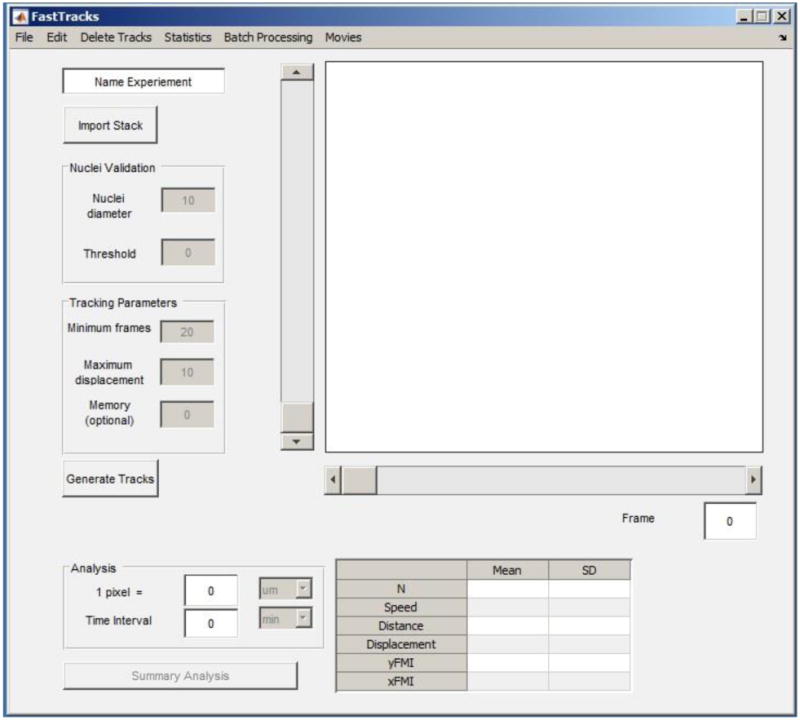
Screenshot of the FastTracks GUI immediately after initializing the program.

Figure 2.

Screenshot showing where to enter the name of the experiment. This name will be appended to exported data generated in FastTracks.

Figure 3.

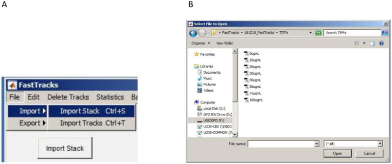
Screenshot showing A) options for importing image stacks and B) the file selection window from which you navigate to image files of interest.

Figure 4.

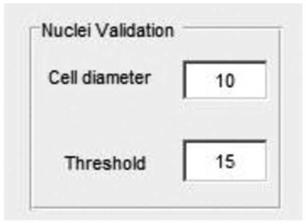
Screenshot showing where to enter the approximate diameter of the nuclei and threshold for the image being evaluated.

Figure 5.

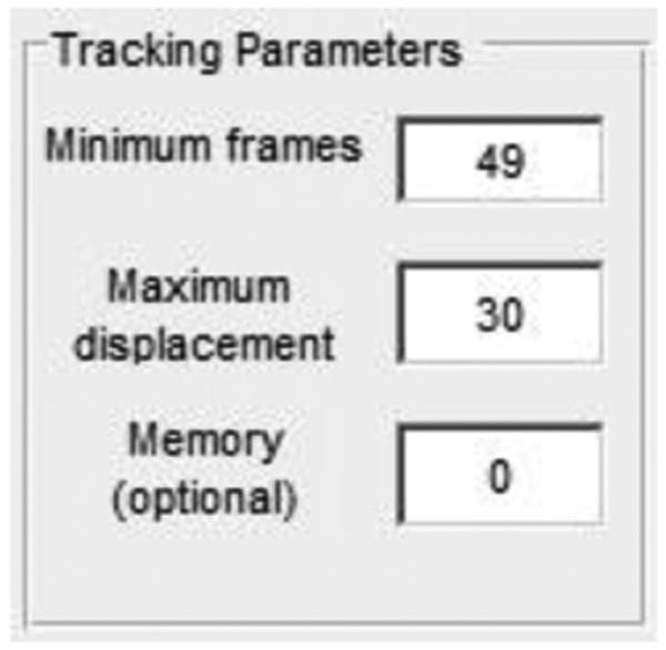
Screenshot showing where to enter Minimum frames, Maximum displacement, and Memory parameters.

Figure 6. Display of cell trajectories overlaid onto the current frame of the time-lapse stack after initiating the Generate Tracks function.

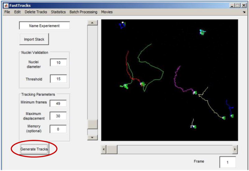
Figure 7. Screenshot showing where to find the Export Tracks option.

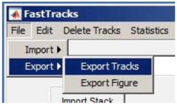
Figure 8.

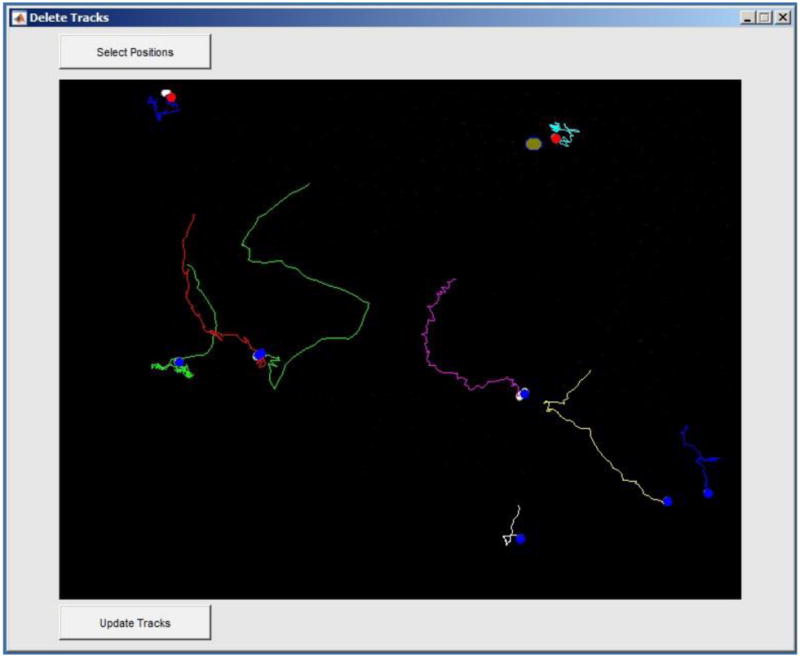
Example Delete Tracks window. Two tracks have been selected to be deleted from the tracks data set as indicated by the red circle that overlays the initial positions of these tracks.

Figure 9.

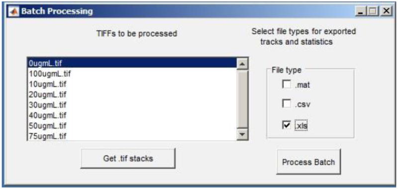
The Batch Processing window features a list box that contains the file names of TIFF documents that will be analyzed. One or more file types containing data of interest can also be exported.

Figure 10. Screen shot showing where to find the ROI Blackout option.

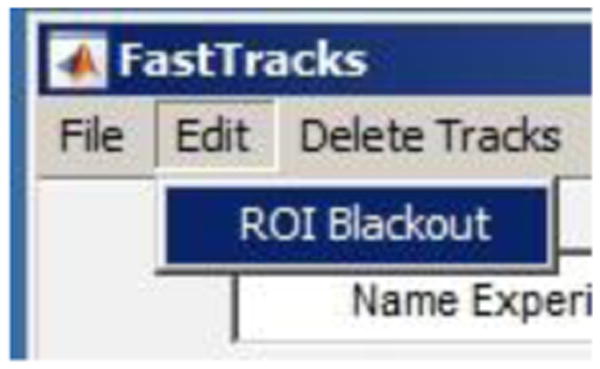
Figure 11.

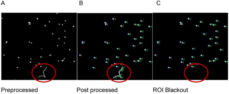
A) The preprocessed image reflects the raw image data that will be imported into the FastTracks program, which in this case contains fluorescent debris. B) Post-processing of the image by setting nuclei parameters may incorrectly identify portions of the debris for tracking. C) Applying the ROI Blackout feature eliminates this region from the image stack, thereby preventing erroneous tracks from being generated.

Figure 12. Screen shot of the Analysis panel on the main GUI window.

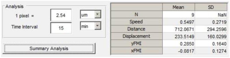
Figure 13.

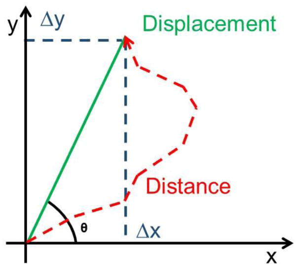
Graphical schematic of a cell trajectory and variables used to report migratory phenotypes.

Figure 14. Screen shot of Export Data window.

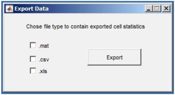
Figure 15.

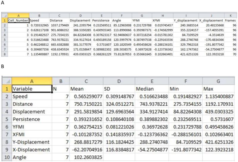
Examples of population and individual cell statistics data. A) The individual cell statistics data set contains a numerical identifier for each cell and includes the cells speed, distance, displacement, persistence, angular displacement, FMI along the X and Y axis, Y-displacement, X-displacement, and the number of frames the cell was tracked (see Figure 13 and Table I for how these values are calculated). B) Population statistics contain the mean, standard deviation, median, minimum and maximum values for the individual cell statistics data set.

Movie 1. Trajectories of a low-density culture.

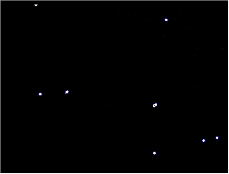
A movie of fluorescently labeled nuclei trajectories from a low density culture of U87 cells imaged for 24 h at 15 min intervals. The trajectories were generated using the following settings: Nuclei diameter = 12, Threshold = 15, Minumum frames = 49, Maximum displacement = 30. (Practice using FastTracks by importing the low_density_culture.tif contained in the downloadable sample_TIFFs folder.)

Movie 2. Trajectories of a high-density culture.

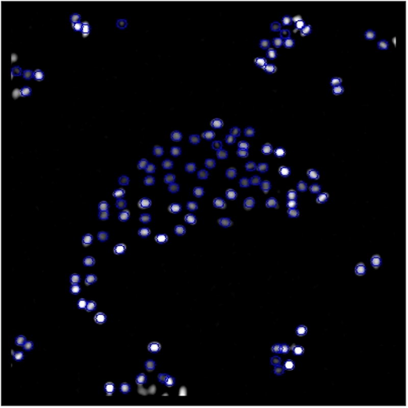
A movie of fluorescently labeled nuclei trajectories from a high density culture of MDCK cells imaged for 4 h at 5 min intervals. The trajectories were generated using the following settings: Nuclei diameter = 10, Threshold = 10, Minumum frames = 20, Maximum displacement = 10. (Practice using FastTracks by importing the high_density_culture.tif contained in the downloadable FastTracks program files.)

Significance Statement.

Manual tracking is a classical technique to obtain data for characterizing cell migration. Unfortunately, manual tracking is a time-consuming and labor-intensive task that can be a prohibitive rate-limiting step when acquiring migratory data. Automated tracking of cell positions in time-lapse movies to obtain cell trajectories represents a significant technical advance for quantitative studies of cell migration. This Unit describes user-friendly methods for automating the acquisition of cell tracks in a rapid, unbiased, and accurate process to facilitate more efficient testing of hypotheses and analyzing data by cell biologists.

Literature Cited

- Cordelieres FP, Petit V, Kumasaka M, Debeir O, Letort V, Gallagher SJ, Larue L. Automated cell tracking and analysis in phase-contrast videos (iTrack4U): development of Java software based on combined mean-shift processes. PLoS One. 2013;8:e81266. doi: 10.1371/journal.pone.0081266. [DOI] [PMC free article] [PubMed] [Google Scholar]
- Crocker JC, Grier DG. Methods of digital video microscopy for colloidal studies. J Colloid Interf Sci. 1996;179:298–310. [Google Scholar]
- Friedl P, Alexander S. Cancer invasion and the microenvironment: plasticity and reciprocity. Cell. 2011;147:992–1009. doi: 10.1016/j.cell.2011.11.016. [DOI] [PubMed] [Google Scholar]
- Hand AJ, Sun T, Barber DC, Hose DR, MacNeil S. Automated tracking of migrating cells in phase-contrast video microscopy sequences using image registration. J Microsc. 2009;234:62–79. doi: 10.1111/j.1365-2818.2009.03144.x. [DOI] [PubMed] [Google Scholar]
- Manzo C, Garcia-Parajo MF. A review of progress in single particle tracking: from methods to biophysical insights. Rep Prog Phys. 2015;78 doi: 10.1088/0034-4885/78/12/124601. [DOI] [PubMed] [Google Scholar]
- Masuzzo P, Van Troys M, Ampe C, Martens L. Taking Aim at Moving Targets in Computational Cell Migration. Trends Cell Biol. 2016;26:88–110. doi: 10.1016/j.tcb.2015.09.003. [DOI] [PubMed] [Google Scholar]
- Mayor R, Theveneau E. The neural crest. Development. 2013;140:2247–2251. doi: 10.1242/dev.091751. [DOI] [PubMed] [Google Scholar]
- Meijering E, Dzyubachyk O, Smal I, van Cappellen WA. Tracking in cell and developmental biology. Semin Cell Dev Biol. 2009;20:894–902. doi: 10.1016/j.semcdb.2009.07.004. [DOI] [PubMed] [Google Scholar]
- Piccinini F, Kiss A, Horvath P. CellTracker (not only) for dummies. Bioinformatics. 2016;32:955–957. doi: 10.1093/bioinformatics/btv686. [DOI] [PubMed] [Google Scholar]
- Rajan SS, Liu HY, Vu TQ. Ligand-bound quantum dot probes for studying the molecular scale dynamics of receptor endocytic trafficking in live cells. ACS Nano. 2008;2:1153–1166. doi: 10.1021/nn700399e. [DOI] [PubMed] [Google Scholar]
- Sako Y, Minoghchi S, Yanagida T. Single-molecule imaging of EGFR signalling on the surface of living cells. Nat Cell Biol. 2000;2:168–172. doi: 10.1038/35004044. [DOI] [PubMed] [Google Scholar]
- Schutz GJ, Kada G, Pastushenko VP, Schindler H. Properties of lipid microdomains in a muscle cell membrane visualized by single molecule microscopy. Embo J. 2000;19:892–901. doi: 10.1093/emboj/19.5.892. [DOI] [PMC free article] [PubMed] [Google Scholar]
- Singer AJ, Clark RA. Cutaneous wound healing. N Engl J Med. 1999;341:738–746. doi: 10.1056/NEJM199909023411006. [DOI] [PubMed] [Google Scholar]