DeepBipolar: Identifying Genomic Mutations for Bipolar Disorder via Deep Learning

Abstract

Bipolar disorder (BD), also known as manic depression, is a brain disorder that affects the brain structure of a patient. It results in extreme mood swings, severe states of depression and over-excitement simultaneously. It is estimated that roughly 3% of the population of the United States (about 5.3 million adults) suffers from BD. Recent research efforts like the Twin studies have demonstrated a high heritability factor for the disorder, making genomics a viable alternative for detecting and treating bipolar disorder, in addition to conventional lengthy and costly post-symptom clinical diagnosis. Motivated by this study, leveraging several emerging deep learning algorithms, we design an end-to-end deep learning architecture (called DeepBipolar) to predict BD based on limited genomic data. DeepBipolar adopts the Deep Convolutional Neural Network (DCNN) architecture that automatically extracts features from genotype information to predict the bipolar phenotype. We participated in the Critical Assessment of Genome Interpretation (CAGI) bipolar disorder challenge and DeepBipolar was considered the most successful by the independent assessor. In this work, we thoroughly evaluate the performance of DeepBipolar and analyze the type of signals we believe could have affected the classifier in distinguishing the case samples from the control set.

I. INTRODUCTION

Bipolar disorder, also known as manic-depressive illness, is a complex genetic disorder, resulting in hysteria or severe states of depression. Medical research reports that bipolar disorder affects close to 5.7 million adults in the United States aged 18 or above (Bipolar disorder statistics). Suicides alone kill 15% to 17% of bipolar disorder patients. Around 51% of the patients are estimated to go untreated due to lack of efficient and effective detection and treatment solutions(Bipolar disorder statistics). Twin studies of BD have yielded estimates of heritability up to 90% (Craddock et al. 2013), the highest among all mental disorders (Shih, Regina A. et al. 2004; Sullivan, Patrick F., et al. 2012). The Psychiatric Genomics Consortium (PGC) (Psychiatric GWAS. 2011) identified 19 genome-wide significant loci for this disorder based on genome-wide association studies. This study was the first significant result identifying genetic BD factors. Motivated by these recent discoveries, Critical Assessment of Genome Interpretation announced the BD exomes challenge, in search of predictor methods for bipolar phenotypes from specific genotypes. As a part of the challenge, we proposed a deep learning based framework (called DeepBipolar) to predict bipolar disorder phenotypes from genotypes.

Deep learning (DL) combines lower-level representations to yield higher-level representations of the input datasets. Unlike conventional/shallow machine learning techniques that require feature engineering, deep learning models learn the features automatically through multiple layers (tens or hundreds of layers) of hierarchical representations, without handcrafted features (Yann LeCun et al. 2015). DL achieved state-of-the-art results in several domains, such as computer vision (Krizhevsky et al. 2012), natural language processing (Tomas Mikolov et al. 2010) and speech recognition (Hinton, G. et al. 2012), with applications in fields such as genomics (Jian Zhou & Olga G. Troyanskaya. 2015) and astronomy (M. Huertas-company et al. 2015) as well. Some commonly used deep learning models include Deep Autoencoders (G. E. Hinton and R. R. Salakhutdinov. 2006), Convolutional Neural Networks (Yann LeCun et al. 2002) and Long Short-term Memory (Hochreiter, Sepp, and Jürgen Schmidhuber. 1997). DeepBipolar leverages the design of convolutional models and performs convolutions with trainable filters/kernels on the input genomic sequences. The convolving kernels move around in a window length across the input sequences, forming feature maps of the input sequences. Additionally, adding further layers of convolution causes the extraction of richer intricate features within the data, resulting in feature maps. Pooling is a common operation applied on these feature maps and is based on spatial invariance in the input dataset. The idea is that key features are more important than their surroundings. Two popular pooling techniques are max pooling and mean pooling.

DeepBipolar combines the state-of-the-art Deep Convolutional Neural Networks with biological indicators to predict these phenotypes. We show that our technique achieved the best accuracy in predicting the diseased group from the control group, while substantially outperforming other conventional machine learning techniques. After elaborating on the framework, we focus on explaining the features learnt by the model to decipher the biological indicators of the disease. Then, through an understanding of the features learnt by the model, we carry out post-analysis studies to identify the key contributors to the disorder. We found that the data could have issues related to sequencing. Identifying these as practices prevalent in the exomes sequencing community, we acknowledge and highlight the drawbacks of such a data preparation. Machine learning algorithms are suitable for identifying features that differentiate between various data points. Traditionally, experiments are designed to minimize any random noise in the data preparation phase to ensure the employed machine learning or statistical methods work on the actual biological indicators of the disorder and less on the artifacts. Therefore, the scope for systematic or batch artifacts is high in genome sequencing studies, based on such approaches that are used to sequence the case and control sets. Furthermore, some cost-effective measures used in genomic communities, say, using a control set of another sequencing study, can introduce artifacts in the datasets that are picked up by the machine learning model. After introducing our framework, we identify the features learnt and design experiments to measure the usability of the exome sequencing SNP for identifying bipolar disorder phenotypes.

II. RELATED WORK

Bipolar disorder studies are based on the structure of the human brain and its activities using Functional Magnetic Resonance Imaging (FMRI) and Positron Emission Tomography (PET) instruments (Bipolar Disorder (NHS)). These studies highlight the smaller size of the prefrontal cortex of the brain in bipolar patients, with the brain activity in such patients being similar to patients suffering from other brain disorders like schizophrenia (Bipolar Disorder (NHS)).

Twin studies of BD show heritability as the most responsible factor causing the disorder (Craddock et al. 2013). This factor is close to 90% and is amongst the highest across all other mental disorders (Shih, Regina A. et al. 2004; Sullivan, Patrick F. et al. 2012). There have been previous studies analyzing the lifetime prevalence of the disorder and the heritability associated with it (Sullivan, Patrick F. et al. 2012), affirming the link between non-genetic factors and bipolar disorder (Alloy, Lauren B. et al. 2005), therefore leading to Genome-Wide Association Studies (GWAS). Studies conducted by the Psychiatric Genomics Consortium (PGC) concluded that there is less than 25% total variance in liability of BD that could be explained by all SNPs (C., Lee & S.H. et al. 2013). This shows that variants that were poorly tagged and missed by GWAS contribute to the risk of Bipolar Disorder (Bodmer, W. and Bonilla, C. 2008; Manolio, T.A. et al. 2009; Cirulli, E.T. and Goldstein, D.B. 2010). These studies prompted BD study using exome sequencing with the bipolar exome challenge, released by CAGI, being one among them.

Various machine learning algorithms have been employed for predicting phenotype from genotype but there are few works in the literature that leverage the remarkable capability of deep neural networks for such tasks. Deep Learning works on spatial invariance between input features, especially convolutional neural networks that are used extensively in computational biology. This model utilizes the sliding window technique to understand the interactions between the SNPs and their context. For various challenging problems like variant interpretation, deep learning algorithms have yielded state-of-the-art results with genome sequences data (Babak Alipanahi et al. 2015; Hui Y. Xiong et al. 2015). During sequencing analysis, a large number of variants poses a greater challenge and carrying out studies on such a large pool of the human population is tedious and expensive. This necessitates higher and superior dimensionality reduction algorithms for machine learning models to work efficiently, and the promise shown by convolutional autoencoders to extract and compose robust features is effective, as shown by previous research (Vincent, Pascal et al. 2008).

III. DEEPBIPOLAR

This section introduces the dataset we worked on the challenge related to the prediction of bipolar phenotype. We also elaborate on our post-result analysis the insight we gained to better understand the data and through our DeepBipolar framework.

A. Datasets

The dataset was provided by The Regents of the University of California under the challenge “Bipolar Exomes” in the Critical Assessment of Genomic Interpretation 4 experiment. The dataset consists of 1000 samples, whose exome sequences are available, and 500 samples of the dataset are labeled to indicate whether the sample belongs to the diseased or the control group. Within the labeled dataset, there is a 50–50 split between the test and the control group. These data samples were randomly sampled from the pool of 1000 samples. The challenge is to predict the labels of the next 500 samples to indicate whether they belong to the diseased or the control group. For target capture and sampling, 60 genes of bipolar disorder were used. Intronic information of 1,422 synaptic genes and NimbleGen SeqCap EZ v2.0 Exome arrays were also utilized (CAGI -4). Additionally, variants with more than 10% missing data or a Hardy-Weinberg disequilibrium value of p less than10⁻⁶ with the genotype of read depth less than 10, or genotype quality less than 20 were excluded (CAGI -4).

B. Data Visualization

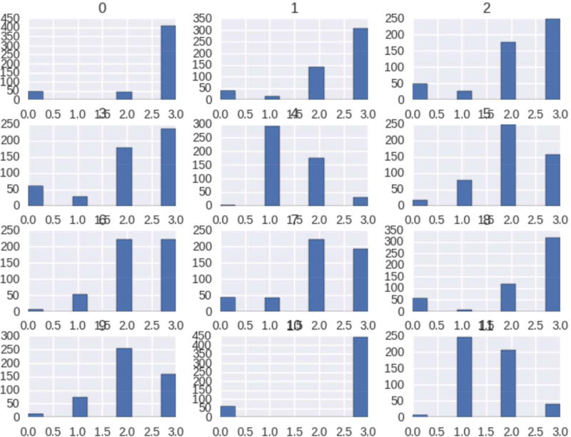
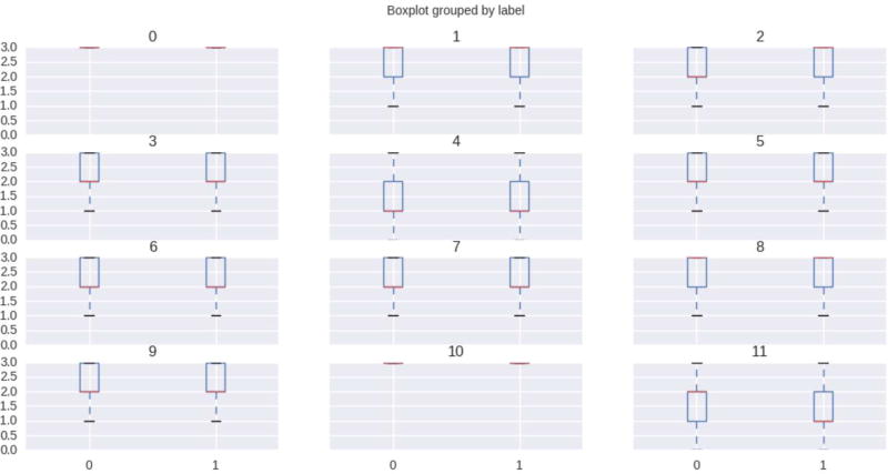
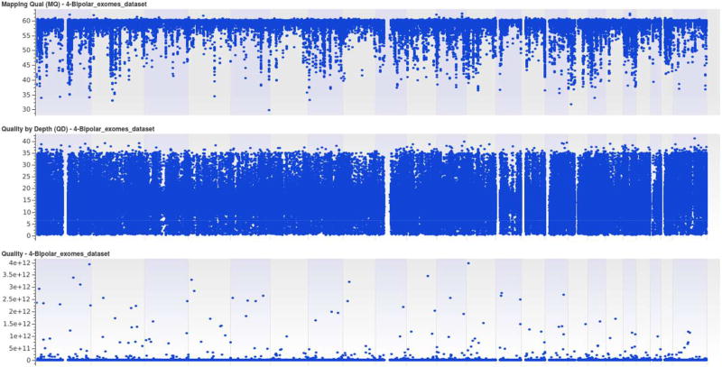
Histograms and box plots are plotted to visualize the distribution of our datasets. It is easier to plot the distribution as all the genotypes in our dataset are unphased and we encode them with the numerical value, as explained in the data preprocessing section. As the number of variants for all the chromosomes is greater than 5e5, we use feature selection to reduce feature dimension. This is achieved through L1-based feature selection with regularization penalty parameter, C = 0.85. This reduces to less than 1% of the total features and we use the top 12 variants for visualization purposes. Figure 1 and Figure 2, are the histogram and box plot respectively for our bipolar datasets. Similarly, Figure 3, summarizes the mapping quality, quality depth and genotype quality for our data sets, without employing any threshold on low-quality variants.

Figure 1. Histogram Plot of Bipolar Datasets.

Figure 1 Shows the histogram plot of our datasets. Histogram are generated using top important feature/variant selection applying L1-based feature selection methods.

Figure 2. Box Plot of Bipolar Datasets.

Figure 2 Shows the box plot of our datasets. Box plot are generated using top important feature/variant selection applying L1-based feature selection methods.

Figure 3. Mapping Quality, Quality Depth and Genotype Quality of Bipolar Datasets.

Figure 3 Shows the data statistics of our bipolar datasets. It summarizes the mapping quality, quality depth and genotype quality of our datasets.

C. Data Preprocessing

The data has the genotype information along with allele depth, read depth and genotype quality. To make the data consumable for deep learning models, we extract the genotype information for each variant that has a genotype quality greater than 50. As convolution works on spatial invariance and there is no ordering between variants across chromosomes, we use convolution within variants belonging to the same chromosome. For all the variants, we had their unphased genotype information, for example, “reference allele” / “alternate allele” 1, “reference allele”/ “alternate allele” 2 etc. To ensure the deep learning models are unbiased and do not favor one genotype over the other, we create one-hot-encoded vectors for all the types of genotypes available. 0/0 is made as 001, 0/1 is made as 010 and so on. This encoding ensures that all the categories are equidistant from each other.

We also separate out variants from each chromosome separately because deep learning networks work on spatial invariance. There is an inherent ordering of variants among each chromosome but there is no such ordering between chromosomes. For this reason, convolution could not be applied over all the chromosomes, and is hence separated. Next, for each of the samples, we feed to our deep learning model all its variants across each chromosome and the target label of 1 or 0, with 1 being the diseased group. For validation purposes, we randomly sample 400 from both the case and the control groups for training and remaining 100 with labels for validation, and later predict the remaining 500 unlabeled test sets using this trained model. In typical optimization algorithms, it is important for the loss function to be computed on both the classes because in an unbalanced dataset, machine learning models tend to favor the bigger class as it reduces the loss. Here, we ensure that it is less likely for our models to learn one-class features better as we have evenly split the training dataset.

D. DeepBipolar Architecture

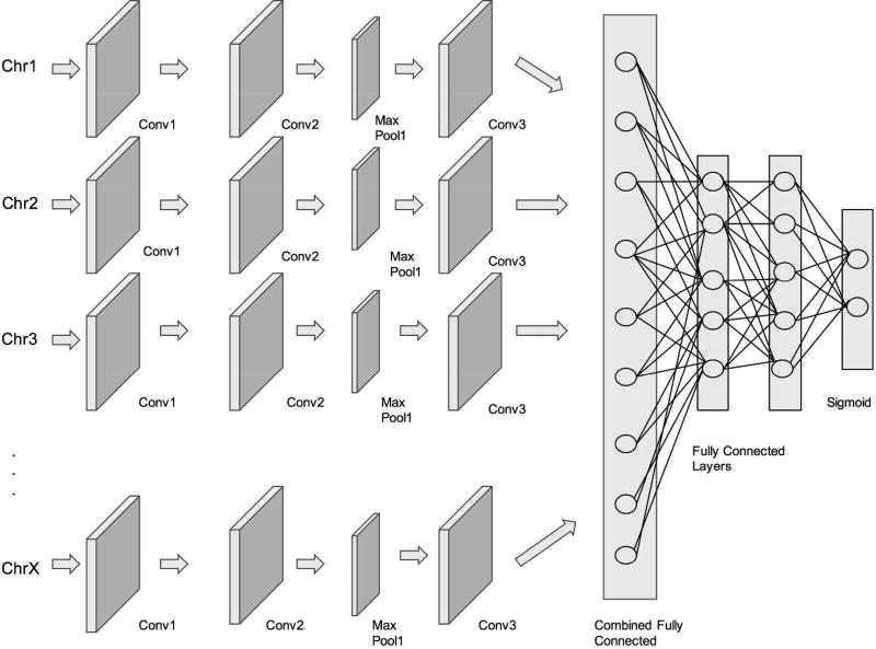
Inspired by state-of-the-art convolutional architectures, the architecture of DeepBipolar takes in a 23-channel input, with each input being the variants of a chromosome starting from 1 to 22 and chromosome X.

The richer and finer interactions between the variants of each chromosome are captured by the 1D convolution and are applied across each channel of input. Figure 4, illustrates our DeepBipolar framework. Specific details of the number of layers of convolution with respect to each channel is obtained from Table I. We have a block of two convolutional layers, followed by a max-pooling layer resulting in sparser feature maps containing only the most important features. In each block, the max-pooling layer is followed by a batch normalization layer that helps in keeping the activation of the neurons in non-saturation regions. This further avoids overfitting the data by regularizing the activations of each max-pooling layer. Next, we combine the feature maps from all the input channels by using a fully connected layer. This fully connected layer is then connected to one other fully connected layer with the final layer being the sigmoidal layer. This sigmoidal layer produces probabilities of output from 0 to 1, with control set belonging to class 0 and diseased group belonging to class 1.

Figure 4. DeepBipolar Architecure.

Figure 4 shows the overall layout diagram of the DeepBipolar architecture. Each chromosome has its own input channel and the features extracted by convolution are later combined in a fully connected layer.

TABLE I. Bipolar CNN Architecture.

Table I provides the individual layer configuration details for the DeepBipolar convolutional neural network architecture.

Chromosome	Layer	Number of Kernel	Kernel Size	Pool Size
Chromosome 1-Chromosome X	Convolution 1	64	60	-
	Convolution 2	64	60	-
	Max Pool 1	-	-	2
	Convolution 4	128	30	-
	Convolution 5	128	30	-
	Max Pool 2	-	-	2
	Fully Connected 1	64	-	-
Combined Layers	Combined Fully Connected 1(Merge Mode: Sum)	128	-	-
	Combined Fully Connected 2	64	-	-
Output Layer	Sigmoid	2	-	-

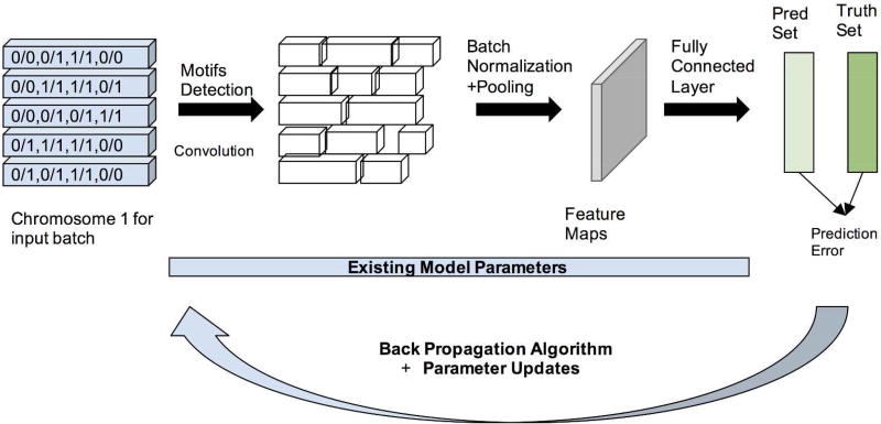
Each neuron consists of ReLU activation to introduce non-linearity in the network. This helps the model get deeper by eliminating the vanishing gradient problem observed with tanh or sigmoid nonlinear activations of neurons. The deep neural network is then trained using gradient descent by standard backpropagation algorithm (Yann LeCun et al. 2015). We use a much quicker version of gradient descent i.e. stochastic gradient descent with a batch size of 32, i.e., the gradient descent happens for all the 32 samples together. This makes the order of input data important and, hence, for this reason, we reshuffle the input training dataset after every epoch. At the end of one epoch over all the batches, we obtained two sets of vectors. The first set of vectors is the value of the predicted classes for all the training samples, and the second set of vectors is the true class of the samples in the training set. Taking these two vector, we calculate the Bernoulli distance by computing the KL divergence. This step provides us with the loss function, representing a distance measure between the predicted and true labels. We then run the next epoch, initializing weights to reduce the loss function obtained in epoch 1. Each epoch runs until the model converges with a patience of 5 epochs, i.e., the training was stopped when the validation accuracy did not improve for more than 5 epochs, usually implying model overfitting (on the training data). Empirically, it takes around 100 epochs to converge with a learning rate of 10⁻⁴ using the Adam optimizer. Training the model end-to-end takes close to 6 hours on Nvidia Tesla M40 servers. In Figure 5, the whole process of training is illustrated by taking Chromosome 1 as an example. The sample process went into all the chromosome channels.

Figure 5. Model Training Workflow of DeepBipolar.

Figure 5 illustrates the working of the DeepBipolar model for input chromosome 1. It consists of generation of feature maps through series of convolution and back propagating the error between the predicted labels and true labels to optimize the loss.

E. Comparison with Conventional Machine Learning Techniques

Apart from convolutional neural networks, we also employ decision trees and random forests techniques for obtaining the classification results. We train 400 samples for training and 100 for validation with the rest of the 500 samples for testing. Accuracy of 0.536 in the case of decision trees and 0.548 for random forests with 10 estimators (default) is recorded. Classification score summary for both the approaches is given in Table II. AUC scores recorded were 0.53 and 0.55 respectively.

Table II. Classification Score Summary for Decision Tree/Random Forest/Convolutional Neural Network.

Table II provides the accuracy metrics of precision, recall and the F1 score for Decision tree/Random forest and DeepBipolar convolutional neural network classifier. Each of the value for each classifier are separated by “/“.

	Precision	Recall	F1-Score	Support
Unaffected-0	0.53/0.53/0.63	0.53/0.73/0.68	0.53/0.62/0.65	249
Bipolar Disorder-1	0.54/0.58/0.66	0.54/0.37/0.61	0.54/0.45/0.63	251
Avg/Total	0.54/0.56/0.64	0.54/0.55/0.64	0.54/0.53/0.64	500

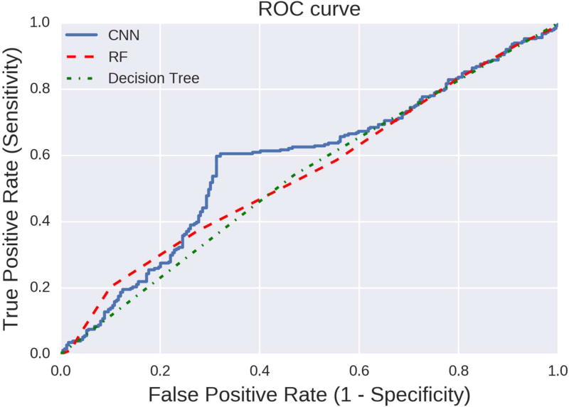
ROC curve for the decision trees and random forests is shown in Figure 6. We applied a threshold of 0.5. Both of these classifiers are able to classify the Bipolar Disorder patient almost equally well as shown in Figure 6. Compared to traditional machine learning techniques, the winning performance results were obtained by using a deep convolutional neural network architecture. The accuracy of the deep convolutional neural network model in predicting both the classes is about 65%. The typically hard nature of the problem might explain such a modest accuracy metric winning the prediction challenge. Table II and Figure 6, illustrate the performance metrics of the convolutional design. Tables II–III describe the accuracy with precision, recall parameters and Figure 6, is the ROC curve for this approach. We applied Scikit-learn (v0.181) and Keras(v1.2.2) Python software packages for these analyses.

Figure 6. ROC Curve of DeepBipolar vs Shallow Machine Learning.

Figure 6 shows the ROC curve for the performance of classifiers based on Logistic regression and Random forest techniques and DeepBipolar convolutional neural network classifier.

TABLE III. Prediction Score for Deepbipolar.

Table III is the confusion matrix for the DeepBipolar architecture.

Class	Predict-Unaffected	Predict-Bipolar Disorder
Unaffected-0	169	80
Bipolar Disorder-1	99	152

F. Performance of Other Competitors

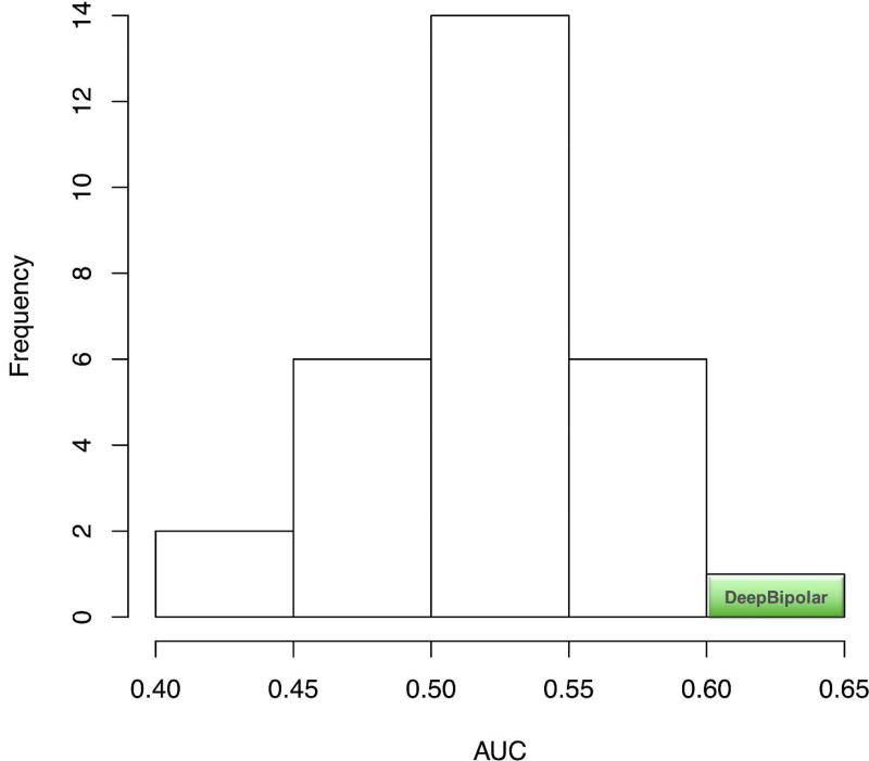
There were 29 submissions overall for the challenge and the Area Under the curve for these submissions is shown in Figure 7 (Alexander Morgan. 2016). The prediction methods had a AUC range from 0.40 to 0.65 with most predictions ranging between 0.5 and 0.55. Our method is in the far right of the AUC curve, having a winning AUC score of 0.65; it achieved the best prediction metric amongst the fellow competitors. This demonstrates the ability of deep convolution based neural networks to understand genomic datasets without handcrafted features. Having introduced the framework and proving its superiority over conventional machine learning model, we proceed to understand the features learnt and the usability of the data in the coming sections.

Figure 7. Performance of DeepBipolar against other Competitors.

Figure 7 plot the performance of all other competitors in the challenges vs DeepBipolar. The result achieved by DeepBipolar classifier is highlighted in green.

G. Post Result Analysis

As a post-result analysis, we want to analyze the features learnt by the DeepBipolar framework and analyze the suitability of the exome sequencing SNPs for prediction of bipolar disorder. The fact that such expensive studies of BD yielded biologists with few credible biological indicators responsible for the disorder made us question whether the features present in the dataset made the machine learning effective. The key question was: “Are there some artifacts that were unknowingly introduced into the dataset during the data preparation process?”. An example of an artifact could be sequencing of the disease group together and using the control set that was sequenced for another study. As mentioned below, we ran two experiments where we restricted the information available to the model by reducing the variants and observed how it classified the samples. By changing the variants as seen by the model, we expected a drop in the classification performance and the experiments below were designed to study it.

1) Experiment-1 Controlling Variants in Each Chromosome

The hypothesis we are trying to answer is, “If we reduce the number of variants in each chromosome channel, does the performance of the machine learning models drop and do these models fail to accurately classify the two classes of sample set?” Essentially, if no changes in the classification ability of the machine learning models are observed, then the machine learning models are most likely picking up some artifacts that differentiate between these classes.

1. We pick only the first 1000 variants of each chromosome.

2. We picked at random 1000 variants of each chromosome.

3. We pick only the last 1000 variants of each chromosome.

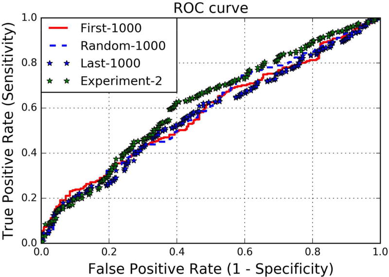
ROC curve for all three cases, along with that of experiment 2 is shown in Figure 8. Prediction score for our 3 experiments are shown in Table IV, where 1st, 2nd and 3rd values correspond to first 1000, random 1000 and last 1000 variant of each chromosome, each separated by ‘/’. The results of all the three techniques of data preprocessing with our machine learning model are identical. The ROC curves indicate the model’s predictions being significantly affected by the absence of the variants across these chromosomes. Therefore, the model needs all the variants to replicate the winning performance at the CAGI challenge. Had there been artifacts present in the dataset, the models might have performed without a drop in the performance and that would have been a consistent signal of case and control sets across the variants and chromosomes.

Figure 8. ROC Curves for Experiment I & II.

Figure 8 plots three ROC curves for the experiments that we performed i.e. giving the DeepBipolar classifier only the first 1000 variants/random 1000 variants and the last 1000 variants across each chromosome as three separate experiments.

TABLE IV. Prediction Score for Experiment-I.

Table IV provides the confusion matrix for DeepBipolar convolutional neural network classifier when the number of variants across each chromose is restricted to first 1000 – random 1000 and last 1000. The “/“ indicate the first value is the metric for the first 1000 variants, the value between two “/“ is the metric for the random 1000 variants and the last value is the metric for the last 1000 variants.

Class	Predict-Unaffected	Predict-Bipolar Disorder
Unaffected-0	137/131/130	112/118/119
Bipolar Disorder-1	114/106/98	137/145/153

2) Experiment-2 Training with Chromosome 1 and 2 / Testing with Chromosome 5,6,7 & 8

In this experiment, we train the deep learning models with variants only from the chromosomes 1 & 2. During the testing time, we show the variants only from chromosomes 5,6,7 and 8. Given that an artifact signal would be consistent, even without showing the model all the chromosomes, the model should be able to replicate the winning performance, i.e. a model that trains with all variants. As we see, there is a huge drop in performance. Any differences that might arise due to sequencing should be uniform across chromosomes and the models would have expected to work similarly well in training on one set of chromosomes and testing on another set. Given the significant drop in performances, the likelihood of the presence of such signals being picked up by the neural network models for classification is quite remote as the performance takes a considerable hit on these experiments.

IV. OBSERVATIONS

We initially suspected the neural networks of picking up signals arising out of different sequencing technologies, but the experimental results suggest otherwise. The experiments were designed to show the presence of signal in the datasets to distinguish the case from the control case. The results from the experiment sufficiently prove the existence of such a signal and have shown that the neural networks are picking up signals that are not differences in sequencing technologies. Given the lack of interpretability with neural networks, we had to rely on the input signal and the changes it effects on the output performance. Given that convolutional neural networks excel at picking interlinked features, the models might be picking up complex patterns across the samples to classify the diseases and rely less on noise. Recently there have been significant advances in interpreting neural networks and, hence, as a future work, we plan to analyze and score each of the variants with respect to its impact on classifying the variants as benign or pathogenic.

V. CONCLUSION

We propose a deep learning based framework called DeepBipolar and analyse the genotype information to predict the bipolar phenotype using convolutional neural networks. The technique described in this paper achieved the winning results in the CAGI-4 bipolar prediction challenge. Given the lack of need for hand-engineering the feature set for classifying the disease samples, such a technique might be a useful tool in computational biology.

References

- 1.Alexander Morgan. Bipolar Assessors presentation, CAGI conference.2016. [Google Scholar]
- 2.Alloy Lauren B, et al. The psychosocial context of bipolar disorder: environmental, cognitive, and developmental risk factors. Clinical psychology review. 2005;25(8):1043–1075. doi: 10.1016/j.cpr.2005.06.006. [DOI] [PubMed] [Google Scholar]
- 3.Babak Alipanahi, Delong Andrew, Weirauch Matthew T, Frey Brendan J. Predicting the sequence specificities of DNA and RNA-binding proteins by deep learning. Nature Biotechnology. 2015 Aug; doi: 10.1038/nbt.3300. [DOI] [PubMed] [Google Scholar]
- 4.Bipolar Disorder (NHS) National Institute of Mental Health and Education portal. https://www.nimh.nih.gov/health/topics/bipolar-disorder/index.shtml.
- 5.Bipolar disorder statistics. http://www.bipolar-lives.com/bipolar-disorder-statistics.html.
- 6.Bodmer W, Bonilla C. Common and rare variants in multifactorial susceptibility to common diseases. Nature genetics. 2008;40:695–701. doi: 10.1038/ng.f.136. [DOI] [PMC free article] [PubMed] [Google Scholar]
- 7.CAGI -4. 2016 https://genomeinterpretation.org/content/4-bipolar-exomes.
- 8.Cirulli ET, Goldstein DB. Uncovering the roles of rare variants in common disease through whole-genome sequencing. Nature reviews Genetics. 2010;11:415–425. doi: 10.1038/nrg2779. [DOI] [PubMed] [Google Scholar]
- 9.Craddock Nick, Jones Ian. Genetics of bipolar disorder. Journal of medical genetics. 1999;36(8):585–594. doi: 10.1136/jmg.36.8.585. [DOI] [PMC free article] [PubMed] [Google Scholar]
- 10.Craddock Nick, Sklar Pamela. Genetics of bipolar disorder. The Lancet. 2013;381(9878):1654–1662. doi: 10.1016/S0140-6736(13)60855-7. [DOI] [PubMed] [Google Scholar]
- 11.Lee C, Ripke SH, Neale S, Faraone BM, Purcell SV, Perlis SM, Mowry RH, Thapar A BJ, Goddard ME, et al. Cross-Disorder Group of the Psychiatric Genomics. Genetic relationship between five psychiatric disorders estimated from genome-wide SNPs. Nature genetics. 2013;45:984–994. doi: 10.1038/ng.2711. [DOI] [PMC free article] [PubMed] [Google Scholar]
- 12.Psychiatric GWAS Consortium Bipolar Disorder Working Group. Large-scale genome-wide association analysis of bipolar disorder identifies a new susceptibility locus near ODZ4. Nature genetics. 2011;43(10):977–983. doi: 10.1038/ng.943. [DOI] [PMC free article] [PubMed] [Google Scholar]
- 13.Sullivan Patrick F, Daly Mark J, O'donovan Michael. Genetic architectures of psychiatric disorders: the emerging picture and its implications. Nature Reviews Genetics. 2012;13(8):537–551. doi: 10.1038/nrg3240. [DOI] [PMC free article] [PubMed] [Google Scholar]
- 14.Hochreiter Sepp, Schmidhuber Jürgen. Long short-term memory. Neural computation. 1997;9(8):1735–1780. doi: 10.1162/neco.1997.9.8.1735. [DOI] [PubMed] [Google Scholar]
- 15.Genome-wide finding. Disorders Share Risk Gene Pathways for Immune, Epigenetic Regulation. 2015 https://www.nimh.nih.gov/news/science-news/2015/disorders-share-risk-gene-pathways-for-immune-epigenetic-regulation.shtml.
- 16.Shih Regina A, Belmonte Pamela L, Zandi Peter P. A review of the evidence from family, twin and adoption studies for a genetic contribution to adult psychiatric disorders. International review of psychiatry. 2004;16(4):260–283. doi: 10.1080/09540260400014401. [DOI] [PubMed] [Google Scholar]
- 17.Sullivan Patrick F, Daly Mark J, O'donovan Michael. Genetic architectures of psychiatric disorders: the emerging picture and its implications. Nature Reviews Genetics. 2012;13(8):537–551. doi: 10.1038/nrg3240. [DOI] [PMC free article] [PubMed] [Google Scholar]
- 18.Hinton GE, Salakhutdinov RR. Reducing the Dimensionality of Data with Neural Networks. Science. 2006 doi: 10.1126/science.1127647. [DOI] [PubMed] [Google Scholar]
- 19.Guze SB, Robins E. Suicide and primary affective disorders. The British journal of psychiatry: the journal of mental science. 1970;117:437–438. doi: 10.1192/bjp.117.539.437. [DOI] [PubMed] [Google Scholar]
- 20.Hinton G, et al. Deep neural networks for acoustic modeling in speech recognition. IEEE Signal Processing Magazine. 2012;29:8297. [Google Scholar]
- 21.Xiong Hui Y, Alipanahi Babak, Lee Leo J, Bretschneider Hannes, Merico Daniele, Yuen Ryan KC, Hua Yimin, Gueroussov Serge, Najafabadi Hamed S, Hughes Timothy R, Morris Quaid, Barash Yoseph, Krainer Adrian R, Jojic Nebojsa, Scherer Stephen W, Blencowe Benjamin J, Frey Brendan J. The human splicing code reveals new insights into the genetic determinants of disease. Science Express, Science. 2015 Jan;347(6218) doi: 10.1126/science.1254806. [DOI] [PMC free article] [PubMed] [Google Scholar]
- 22.Jian Zhou, Troyanskaya Olga G. Predicting the Effects of Noncoding Variants with Deep learning-based Sequence Model. Nature Methods. 2015 doi: 10.1038/nmeth.3547. [DOI] [PMC free article] [PubMed] [Google Scholar]
- 23.Krizhevsky A, Sutskever I, Hinton G. ImageNet classification with deep convolutional neural networks. Proc. Advances in Neural Information Processing Systems. 2012;25:10901098. [Google Scholar]
- 24.Manolio TA, Collins FS, Cox NJ, Goldstein DB, Hindorff LA, Hunter DJ, McCarthy MI, Ramos EM, Cardon LR, Chakravarti A, et al. Finding the missing heritability of complex diseases. Nature. 2009;461:747–753. doi: 10.1038/nature08494. [DOI] [PMC free article] [PubMed] [Google Scholar]
- 25.Merikangas KR, Akiskal HS, Angst J, Greenberg PE, Hirschfeld RM, Petukhova M, Kessler RC. Lifetime and 12-month prevalence of bipolar spectrum disorder in the National Comorbidity Survey replication. Archives of general psychiatry. 2007;64:543–552. doi: 10.1001/archpsyc.64.5.543. [DOI] [PMC free article] [PubMed] [Google Scholar]
- 26.Huertas-company M, gravet R, Cabrera-Vives G, Pérez-González PG, Kartaltepe JS, Barro G, Bernardi M, Mei S, Shankar F, Dimauro P, Bell EF, Kocevski D, Koo DC, Faber SM, Mcintosh DH. A catalog of visual-like morphologies in the 5 candels fields using deep learning. Astrophysical Journal 2015 [Google Scholar]
- 27.Psychiatric, G.C.C.C. Cichon S, Craddock N, Daly M, Faraone SV, Gejman PV, Kelsoe J, Lehner T, Levinson DF, Moran A, et al. Genome wide association studies: history, rationale, and prospects for psychiatric disorders. The American journal of psychiatry. 2009;166:540–556. doi: 10.1176/appi.ajp.2008.08091354. [DOI] [PMC free article] [PubMed] [Google Scholar]
- 28.Schizophrenia Working Group of the Psychiatric Genomics, C. Biological insights from 108 schizophrenia-associated genetic loci. Nature. 2014;511:421–427. doi: 10.1038/nature13595. [DOI] [PMC free article] [PubMed] [Google Scholar]
- 29.Tomas Mikolov, Karafiat Martin, Burget Luka, Cernock Jan Honza, Khudanpur Sanjeev. Recurrent neural network based language model. Interspeech 2010 [Google Scholar]
- 30.Vincent Pascal, et al. Proceedings of the 25th international conference on Machine learning. ACM; 2008. Extracting and composing robust features with denoising autoencoders. [Google Scholar]
- 31.Yann LeCun, Bottou Leon, Bengio Yoshua, Haffner Patrick. Gradient-Based Learning Applied to Document Recognition. Proceedings of the IEEE 2002 [Google Scholar]
- 32.Yann LeCun, Bengio Yoshua, Hinton Geoffrey. Deep Learning Review. Nature. 2015 doi: 10.1038/nature14539. [DOI] [PubMed] [Google Scholar]