

Abstract
A concern for researchers planning multisite studies is that scanner and T1-weighted sequence-related biases on regional volumes could overshadow true effects, especially for studies with a heterogeneous set of scanners and sequences. Current approaches attempt to harmonize data by standardizing hardware, pulse sequences, and protocols, or by calibrating across sites using phantom-based corrections to ensure the same raw image intensities. We propose to avoid harmonization and phantom-based correction entirely. We hypothesized that the bias of estimated regional volumes is scaled between sites due to the contrast and gradient distortion differences between scanners and sequences. Given this assumption, we provide a new statistical framework and derive a power equation to define inclusion criteria for a set of sites based on the variability of their scaling factors. We estimated the scaling factors of 20 scanners with heterogeneous hardware and sequence parameters by scanning a single set of 12 subjects at sites across the United States and Europe. Regional volumes and their scaling factors were estimated for each site using Freesurfer’s segmentation algorithm and ordinary least squares, respectively. The scaling factors were validated by comparing the theoretical and simulated power curves, performing a leave-one-out calibration of regional volumes, and evaluating the absolute agreement of all regional volumes between sites before and after calibration. Using our derived power equation, we were able to define the conditions under which harmonization is not necessary to achieve 80% power. This approach can inform choice of processing pipelines and outcome metrics for multisite studies based on scaling factor variability across sites, enabling collaboration between clinical and research institutions.
1. Introduction
The pooled or meta-analysis of regional brain volumes derived from T1-weighted MRI data across multiple sites is reliable when data is acquired with similar acquisition parameters [1, 2, 3]. The inherent scanner- and sequence-related noise of MRI volumetrics under heterogeneous acquisition parameters has prompted many groups to standardize protocols across imaging sites [1, 4, 5]. However, standardization across multiple sites can be prohibitively expensive and requires a significant effort to implement and maintain. At the other end of the spectrum, multisite studies without standardization can also be successful, albeit with extremely large sample sizes. The ENIGMA consortium, for example, combined scans of over 10,000 subjects from 25 sites with varying field strengths, scanner makes, acquisition protocols, and processing pipelines. The unusually large sample size enabled this consortium to provide robust phenotypic traits despite the variability of non-standardized MRI volumetrics and the power required to run a genome wide association study (GWAS) to identify modest effect sizes [6]. These studies raise the following question: Is there a middle ground between fully standardizing a set of MRI scanners and recruiting thousands of subjects across a large number of sites? Eliminating the harmonization requirement for a multisite study would facilitate inclusion of retrospectively acquired data and data from sites with ongoing longitudinal studies that would not want to adjust their acquisition parameters.
Towards this goal, there is a large body of literature addressing the correction of geometric distortions that result from gradient non-linearities. These corrections fall into two main categories: phantom-based deformation field estimation and direct magnetic field gradient measurement-based deformation estimation, the latter of which requires extra hardware and spherical harmonic information from the manufacturer [7]. Calibration phantoms, such as the Alzheimer’s Disease Neuroimaging Initiative (ADNI) [8] and LEGO® phantoms [9], have been used by large multisite studies to correct for these geometric distortions, which also affect regional volume measurements. These studies have outlined various correction methods that significantly improve deformation field similarity between scanners. However, the relationship between the severity of gradient distortion and its effect on regional volumes, in particular, remains unclear. In the case of heterogeneous acquisitions, correction becomes especially difficult due to additional noise sources. Gradient hardware differences across sites are compounded with contrast variation due to sequence parameter changes. In order to properly evaluate the reproducibility of brain segmentation algorithms, these phantoms should resemble the humain brain in size, shape, and tissue distribution. Droby and colleagues evaluated the stability of a post-mortem brain phantom and found similar reproducibility of volumetric measurements to that of a healthy control [10]. In this study, we propose to measure between-site bias through direct calibration of regional volumes by imaging 12 common healthy controls at each site. Quantifying regional bias allows us to overcome between-site variability by increasing sample size to an optimal amount, rather than employing a phantom-based voxel-wise calibration scheme that corrects both contrast differences and geometric distortions.
We hypothesized that all differences in regional contrast and geometric distortion result in regional volumes that are consistently and linearly scaled from their true value. For a given region of interest (ROI), two mechanisms simultaneously impact the final boundary definition: (1) gradient nonlinearities cause distortion and (2) hardware (including scanner, field strength, and coils) and acquisition parameters modulate tissue contrast. Based on the results of Tardiff and colleagues, who found that contrast-to-noise ratio and contrast inhomogeneity from various pulse sequences and scanner strengths cause regional biases in VBM[11, 12], we hypothesized that each ROI will scale differently at each site. Evidence for this scaling property can also be seen in the overall increase of gray matter volume and decrease of white matter volume of the ADNI-2 compared to the ADNI-1 protocols despite attempts to maintain compatibility between these protocols [13]. It was also observed that hippocampal volumes were 1.17% larger on 3T scanners compared to the 1.5T scanners in the ADNI study [14]. By imaging 12 subjects in 20 different scanners using varying acquisition schemes, we were able to estimate the scaling factor for each regional volume at each site. We also defined a framework for calculating the power of a multisite study as a function of the scaling factor variability between sites. This enables us to power a cross-sectional study, and to outline the conditions under which harmonization could be replaced by sample size optimization. This framework can also indicate which regional volumes are sufficiently reliable to investigate using a multisite approach.
Regional brain volumes are of interest in most neurological conditions, including healthy aging, and typically indicates the degree of neuronal degeneration. In this study, we investigate a number of well-defined regional brain volumetrics related to multiple sclerosis disease progression. Even though focal white matter lesions seen on MRI largely characterize multiple sclerosis (MS), lesion volumes are not strongly correlated with clinical disability [15, 16, 17]. Instead, global gray matter atrophy correlates better with clinical disability (for a review, see [18]), along with white matter volume, to a lesser extent [19]. In addition, regional gray matter atrophy measurements, such as thalamus [20, 21, 22, 23] and caudate [24, 25] volumes, appear to be better predictors of disability [26, 27, 28, 29].
2. Theory
Linear mixed models are common in modeling data from multisite studies because metrics derived from scanner, protocol, and population heterogeneity may not have uncorrelated error terms when modeled in a general linear model (GLM), which violates a key assumption [30]. In fact, Fennema-Notestine and colleagues found that a mixed model, with scanner as a random effect, outperformed pooling data via GLM[31] on a study on hippocampal volumes and aging. Since we are only interested in the effect of scanner-related heterogeneity, we assume that the relationship between the volumetrics and clinical factors of interest are the same at each site. This causes error terms to cluster by scanner and sequence type due to variation in field strengths, acquisition parameters, scanner makes, head coil configurations, and field inhomogeneities, to name a few [1]. Linear mixed models, which include random effects and hierarchical effects, appropriately integrate observation-level data based on their clustering characteristics [30]. The model we propose in this study is similar to a mixed model, with a multiplicative effect instead of an additive effect. Our goal is to incorporate an MRI bias-related term in our model in order to optimize sample sizes.
We first defined the true, unobserved model for subject i at site j as:
| (1) |
Where Ui,j is the unobserved value of the regional brain volume of interest (without any effects from the scanner), and β00, β10 and β20 are the true, unobserved, effect sizes. The covariates are Zi,j, residuals are εi,j, and the contrast vector, Xi,j, is given the weights Xhigh, Xlow = 0.5, −0.5 so that β10 is computed as the average difference between the high and low groups. For this derivation we assume an equal number of subjects observed at each site in the high and low groups with balanced covariates. ε is normally distributed with mean 0 and standard deviation σ0.
We defined a site-level model using the notation of [32], to express the relationship between a brain metric that is scaled by aj as Yi,j = aj * Uij and high or low disease group Xi,j for subject i = 1, …, n at site j as
| (2) |
The site mean, disease effect, and covariate effect randomly vary between sites so the intercept and slope coefficients become dependent variables [32] and we assume:
| (3) |
where the true underlying coefficient, βk,0 for k = 0, 1, 2 is scaled randomly by each site. The major contributors to brain structure region of interest (ROI) boundary variability are contrast differences and gradient distortions, both of which adjust the boundary of the whole ROI rather than add a constant term. To reflect this property, we modeled the systematic error from each MRI sequence as a multiplicative (Yi,j = aj * Yi) rather than additive (Yij = Yi + aj) error term. Similarly, the residual term is also scaled by site, , and the scaling factor, aj, is sampled from a normal distribution with mean μa and variance .
| (4) |
For identifiability, let μa = 1. The mean disease effect estimate, β1,j is defined as the mean brain metric volume difference in the high and low groups.
| (5) |
The unconditional variance of the disease effect estimate at site j is can be written in terms of the unobserved difference between groups before scaling, DU,j = DY,j/aj:
| (6) |
Where we are assuming that DU,j and aj are independent, meaning that MRI-related biases are independent of the biological effects being studied. For the derivation of this formula, see the Appendix. Given the distribution of scaling factors and the variance of the true disease effect, , the equation simplifies to
| (7) |
We standardize the equation by defining the coefficient of variability for the scaling factors as , and the standardized true effect size as .
| (8) |
Finally, the coefficients are averaged over J sites to produce the overall estimate , and
| (9) |
Note that this estimator is asympototically normally distributed when the number of centers, J, is fixed, because it is the average of asymptotically normal estimators. When the number of subjects per site is not equal, the maximum likelihood estimator is the average of the site-level estimates weighted by the standard error, and this is shown in the Appendix. The variance of the overall estimate can be expressed as
| (10) |
In order to test the average disease effect under the null hypothesis that β1 = 0, the non-central F distribution, F(1, J − 1; λ) [32] is applied, with the non-centrality parameter defined as
| (11) |
Figure 1 shows power curves for small to medium effect sizes (δ = 0.2, 0.3, defined in [32]), and a false positive rate of α = 0.002, which allows for 25 comparisons under Bonferroni correction, where the corrected α = 0.05. Power increases for larger λ and maximizes at as CVa approaches 0. In this case, the power equation is dominated by the total number of subjects, as is the case for the GLM. However, even as the number of subjects per site, n, approaches infinity and for non-negligible CVa, λ is still bounded by . At this extreme, the power equation is largely influenced by the number of sites. This highlights the importance of the site-level sample size (J) in addition to the subject-level sample size (n) for power analyses, especially when there is larger variability between sites for metrics of interest. In the methods section, the acquisition protocols and the standard processing pipelines that were used to calculate CVa values of relevant regional brain volumes for MS are described, though this framework could be applied to any MRI derived metric.
Figure 1.

A. Power contours for total number of subjects (nJ) over various effect sizes (d), p= 0.002, CVa = 5%. B. # of sites required for effect sizes and # subjects per site (n). C effect of CVa on # sites for various effect sizes, where n = 200 subjects per site
We emphasize that the use of phantom subjects does not directly contribute to the power equation in Figure 1, as it does not account for any sort of calibration or scaling. However, it requires an estimate for CVa, which is the variability of scaling biases between sites. The goal of this study is to provide researchers with estimates of CVa from our set of calibration phantoms and our set of non-standardized MRI acquisitions. For a standardized set of scanners, the values of CVa may be considered an upper bound.
3. Methods
3.1. Acquisition
T1-weighted 3D-MPRAGE images were acquired from 12 healthy subjects (3 Male, 9 Female, ages 24–57) in 20 scanners across Europe and the United States. Institutional approval was acquired and signed consent was obtained for each subject at each site. These scanners varied in make and model, including all three major manufacturers: Siemens, GE, Philips. Two scans were acquired from each subject, where the subject got out of the scanner between scans for a couple minutes, and was repositioned and rescanned by the scanning technician of that particular site. Previously, Jovicich and colleagues showed that reproducible head positioning along the z axis significantly reduced image intensity variability across sessions [3]. By repositioning in our study, a realistic measure of test-retest variability, which includes the repositioning consistency of each site’s scanning procedure, was captured. Because gradient distortion effects correspond to differences in z-positioning [9], the average translation in the Z-direction between the two runs of each subject at each site was estimated with a rigid body registration.
Tables 1 through 4 show the acquisition parameters for all 20 scanners. Note that the definitions of repetition time (TR), inversion time (TI) and echo time (TE) vary by scanner make. For example, the TR in a Siemens scanner is the time between preparation pulses, while for Philips and GE, the TR is the time between excitation pulses. We decided to report the parameters according to the scanner make definition, rather than trying to make them uniform, because slightly different pulse programming rationales would make a fair comparison difficult. In addition, a 3D-FLASH sequence (TR=20ms, TE=4.92ms, flip angle=25 degrees, resolution=1mm isotropic) was acquired on healthy controls and MS patients at site 12, in order to compare differences in scaling factor estimates between patients and healthy controls.
Table 1.
Top: Acquisition parameters for the four 1.5T scanners. Si = Siemens, Ph = Philips, GE= General Electric. Bottom: Test-retest reliabilities for selected ROIs, processed by Freesurfer. The ROIs are gray matter volume (GMV), subcortical gray matter volume (scGMV), cortex volume (cVol), cortical white matter volume (cWMV), and the volumes of the lateral ventricle (LV), amygdala (Amyg), thalamus (Thal), hippocampus (Hipp), caudate (Caud), and finally the estimated total intracranial volume (eTIV). Test-retest reliability is computed as within-site ICC(1,1).
| 1 | 2 | 3 | 4 | |
|---|---|---|---|---|
| TR (ms) | 8.18 | 7.10 | 2130 | 2080 |
| TE (ms) | 3.86 | 3.20 | 2.94 | 3.10 |
| Strength (T) | 1.50 | 1.50 | 1.50 | 1.50 |
| TI (ms) | 300 | 862.90 | 1100 | 1100 |
| Flip Angle (°) | 20 | 8 | 15 | 15 |
| Make | GE | Ph | Si | Si |
| Voxel Size (mm) | .94×.94×1.2 | 1×1×1 | 1×1×1 | .97×.97×1 |
| Distortion Correction | N | N | N | Y |
| Parallel Imaging | - | 2 | 2 | - |
| FOV (mm) | 240×240×200 | 256×256×160 | 256×256×176 | 234×250×160 |
| Read Out Direction | HF | AP | HF | HF |
| Head coil # channels | 2* | 8 | 20 | 12 |
| Model | Signa LX | Achieva | Avanto | Avanto |
| OS | 11x | 2.50 | VD13B | B17A |
| Acq. Time (min) | 06:24 | 05:34 | 04:58 | 08:56 |
| orientation | sag | sag | sag | sag |
| # scans | 24/24 | 24/24 | 24/24 | 18/18 |
|
| ||||
| Amyg (L) | .93 | .89 | .61 | .96 |
| Amyg (R) | .93 | .90 | .83 | .88 |
| Caud (L) | .96 | .96 | .98 | .99 |
| Caud (R) | .96 | .97 | .90 | .96 |
| GMV | .96 | .99 | .98 | .99 |
| Hipp (L) | .94 | .95 | .89 | .93 |
| Hipp (R) | .93 | .91 | .94 | .95 |
| Thal (L) | .77 | .93 | .59 | .82 |
| Thal (R) | .91 | .90 | .76 | .82 |
| cVol | .95 | .99 | .97 | .99 |
| cWMV | .99 | 1 | .99 | .99 |
| eTIV | 1 | 1 | 1 | 1 |
| scGMV | .98 | .97 | .98 | .93 |
signifies a quadrature coil
Table 4.
Top: Acquisition parameters for 3T Siemens (Si) Trio scanners. Bottom: Test-retest reliabilities for selected ROIs, processed by Freesurfer. The ROIs are gray matter volume (GMV), subcortical gray matter volume (scGMV), cortex volume (cVol), cortical white matter volume (cWMV), and the volumes of the lateral ventricle (LV), amygdala (Amyg), thalamus (Thal), hippocampus (Hipp), caudate (Caud), and finally the estimated total intracranial volume (eTIV). Test-retest reliability is computed as within-site ICC(1,1)
| 16 | 17 | 18 | 19 | 20 | |
|---|---|---|---|---|---|
| TR (ms) | 2300 | 2150 | 1900 | 1900 | 1800 |
| TE (ms) | 2.98 | 3.40 | 3.03 | 2.52 | 3.01 |
| Strength (T) | 3 | 3 | 3 | 3 | 3 |
| TI (ms) | 900 | 1100 | 900 | 900 | 900 |
| Flip Angle (°) | 9 | 8 | 9 | 9 | 9 |
| Make | Si | Si | Si | Si | Si |
| Voxel Size (mm) | 1×1×1 | 1×1×1 | 1×1×1 | 1×1×1 | .86×.86×.86 |
| Distortion Correction | N | N | N | N | N |
| Parallel Imaging | 2 | 2 | 2 | 2 | 2 |
| FOV (mm) | 256×256×176 | 256×256×192 | 256×256×176 | 256×256×192 | 220×220×179 |
| Read Out Direction | HF | RL | AP | FH | FH |
| Head coil # channels | 12 | 12 | 12 | 32 | 32 |
| Model | Trio | Trio | Trio | Trio | Trio |
| OS | MRB17 | VB17 | VB17A | VB17 | MRB19 |
| Acq. Time (min) | 05:03 | 04:59 | 04:26 | 05:26 | 06:25 |
| orientation | sag | ax | sag | sag | sag |
| # scans | 24/24 | 23/24 | 23/24 | 24/24 | 24/24 |
|
| |||||
| Amyg (L) | .55 | .88 | .77 | .88 | .91 |
| Amyg (R) | .85 | .93 | .81 | .94 | .93 |
| Caud (L) | .99 | .95 | .97 | .97 | .97 |
| Caud (R) | .97 | .92 | .98 | .91 | .95 |
| GMV | .99 | .99 | .98 | .99 | 1 |
| Hipp (L) | .71 | .96 | .94 | .93 | .96 |
| Hipp (R) | .94 | .94 | .92 | .83 | .96 |
| Thal (L) | .45 | .85 | .80 | .80 | .88 |
| Thal (R) | .61 | .95 | .85 | .96 | .79 |
| cVol | .99 | .98 | .96 | .99 | 1 |
| cWMV | 1 | .99 | .99 | 1 | 1 |
| eTIV | .97 | 1 | 1 | 1 | 1 |
| scGMV | .98 | .98 | .98 | .98 | .98 |
3.2. Processing
A neuroradiologist reviewed all images to screen for major artifacts and pathology. The standard Freesurfer [33] version 5.3.0 cross-sectional pipeline (recon-all) was run on each site’s native T1-weighted protocol, using the RedHat 7 operating system on IEEE 754 compliant hardware. Both 1.5T and 3T scans were run with the same parameters (without using the −3T flag), meaning that the non-uniformity correction parameters were kept at the default values. All Freesurfer results were quality controlled by evaluating the cortical gray matter segmentation and checking the linear transform to MNI305 space which is used to compute the estimated total intracranial volume [34]. Scans were excluded from the study if the cortical gray matter segmentation misclassified parts of the cortex, or if the registration to MNI305 space was grossly innaccurate. Three scans were excluded for misregistration. Two exclusions were because of data transfer errors. Because of time constraints, some subjects were not able to be scanned. One of the 12 subjects could not travel to all the sites, and that subject was replaced by another of the same age and gender. The details of this are provided in the supplemental materials and the total number of scans is shown in tables 1 – 4. 46 Freesurfer ROIs, including the left and right subcortical ROIs, from the aparc.stats tables, were studied. In this study we report on the ROIs relevant to the disease progression of MS, which include the gray matter volume (GMV), subcortical gray matter volume (scGMV), cortex volume (cVol), cortical white matter volume (cWMV), and the volumes of the lateral ventricle (LV), amygdala (amyg), thalamus (thal), hippocampus (hipp), caudate (caud). The remaining ROIs are reported in the supplemental materials.
Test-retest reliability, defined as ICC(1,1) [35], was computed across each site and protocol for the selected metrics using the “psych” package in R [36]. The between-site ICC(2,1) values were computed following the procedure from previous studies on multisite reliability [35, 1]. Variance components were calculated for a fully crossed random effects model for subject, site, and run using the “lme4” package in R. Using the variance components, between site ICC was defined as
| (12) |
and an overall within-site ICC was defined as
| (13) |
Scaling factors between sites were estimated using ordinary least squares from the average of the scan-rescan volumes, referenced to average scan-rescan volumes from the UCSF site. The OLS was run with the intercept fixed at 0. CVa for each metric was calculated from the sampling distribution of scaling factor estimates â as follows:
| (14) |
3.3. Scaling Factor Validation
Scaling factor estimates were validated under the assumption of scaled, systematic error, in 2 ways: first, by simulating power curves that take into account the uncertainty of the scaling factor estimate, and second, by a leave-one-out calibration. For the simulation, we generate data for each of the 20 sites included in this study. Subcortical gray matter volumes (scGMV) for each site were generated for two subject groups based on a small standardized effect size (Cohen’s d) of 0.2, which reflects the effect sizes seen in genomics studies. Age and gender were generated as matched covariates, where age was sampled from a normal distribution with mean and standard deviation set at 41 and 10 years, respectively. Gender was sampled from a binomial distribution with a probability of 60% female to match typical multiple sclerosis cohorts.
Coefficients were set on the intercept as 63.135 cm3, β10 as −.95 cm3, covariates ZAge as −.25 cm3/year and ZGender as 4.6 cm3. scGM volumes were generated in a linear model using these coefficients and additional noise was added from the residuals, which were sampled from a normal distribution with zero mean and standard deviation 5.03 cm3. Next, the scGM volumes were scaled by each site’s calculated scaling factor and gaussian noise from the residuals of the scaling factor fit of that particular site were added.
| (15) |
The simulated dataset of each individual site was modeled via OLS, and an F score on XGroup was calculated following our proposed statistical model:
| (16) |
A power curve was constructed by running the simulation 5000 times, where power for a particular p-value was defined as the average number of F values greater than the critical F for a set of false positive rates ranging from 1e−4 – 1e−2. The critical F was calculated with degrees of freedom of the numerator and denominator as 1 and 19 respectively. The simulated power curve was compared to the derived theoretical power curve to evaluate how scaling factor uncertainty influences power estimates. If the scaling factors of each site, which were calculated from the 12 subjects, were not accurate, then the added residual noise from the scaling factor estimate would result in the simulated power curve deviating largely from the theoretical curve.
The scaling factors were also validated by calibrating the regional volumes of each site in a leave-one-out cross-validation. The calibrated volume for a particular subject i and site j was scaled by the scaling factor estimated from all subjects excluding subject i. Within- and between-site ICC’s were calculated for the calibrated volumes. If the scaling factor estimates were inaccurate, the between-site ICCs of calibrated regional volumes would be worse than the between-site ICCs of the original regional volumes. Additionally, the between-site ICC’s after calibration should be similar to those found for harmonized studies, such as [1].
Finally, to address the concern about whether these scaling factors could apply to a disease population, we calculated scaling factors from 12 healthy controls and 14 MS patients between 2 different sequences (3D-MPRAGE versus 3D-FLASH) at the UCSF scanner (site 12). The patients had a mean age of 51 years with standard deviation of 11 years, mean disease duration of 15 years with a standard deviation of 12 years, and mean Kurtzke Expanded Disability Status Scale (EDSS) [37] score of 2.8 with a standard deviation of 2.2.
The accuracy of our scaling factor estimates depends on the accuracy of tissue segmentation, but the lesions in MS specifically impact white matter and pial surface segmentations. Because of the effect of lesions on Freesurfer’s tissue classification, all images were manually corrected for lesions on the T1-weighted images by a neurologist after editing by Freesurfer’s quality assurance procedure, which included extensive topological white matter corrections, white matter mask edits, and pial edits on images that were not lesion filled. These manual edits altered the white matter surface so that white matter lesions were not misclassified as gray matter or non-brain tissue. The errors in white matter segmentations most typically occurred at the border of white matter and gray matter and around the ventricles. The errors in pial surface segmentations most typically occurred near the eyes (orbitofrontal) and the superior frontal or medial frontal lobes. Images that were still misclassified after thorough edits were removed from the analysis, because segmentations were not accurate enough to produce realistic scaling factor estimates.
4. Results
Scan-rescan reliability for the 20 scanners is shown in tables 1 through 4. The majority of scan-rescan reliabilities were greater than 80% for the selected Freesurfer-derived volumes, which included gray matter volume (GMV), cortical white matter volume (cWMV), cortex volume (cVol), lateral ventricle (LV), thalamus (thal), amygdala (amyg), caudate (caud), hippocampus (hipp), and estimated total intracranial volume (eTIV). However, the thalamus at sites 3 and 16 had low scan-rescan reproducibility, below 70%. The left hippocampus and amygdala at site 5 were also below 70%, and the left amygdala at site 16 was also low, at 55%. In addition, the average translation in the Z-direction across all sites was 3.5mm±3.7mm, which falls within the accuracy range reported by [9]. The repositioning Z-translation measurements for each site separately is reported in the supplemental materials.
Between- and within-site ICC’s are plotted with the calibrated ICC’s in Figure 2. The between-site ICC’s of the 46 ROIs improved, with the exception of the right lateral ventricle, which did not change after calibration, and the fifth ventricle, which had very low scanrescan reliability, and is shown in the supplemental materials. The within-site ICC’s of the thalamus, hippocampus, and amygdala decreased slightly after calibration. Both calibrated and uncalibrated within-site ICC’s were greater than 90% for the MS related ROIs listed in this paper. For the full set of within- and between- site ICC’s of the Freesurfer aseg regions, see the Supplemental Materials.
Figure 2.

Leave-one-out calibration improvement on within- (WI) and between- (BW) site ICCs for gray matter volume (GMV), subcortical gray matter volume (scGMV), cortex volume (cVol), cortical white matter volume (cWMV), lateral ventricle (LV), Thalamus (Thal), Hippocampus (Hipp), Amygdala (Amyg), Caudate (Caud)
Simulation results are shown in Figure 3. The simulated and theoretical curves align closely when power is equal to 80%, but the simulated curve is slightly lower than the theoretical curve for power below 80%. This is probably due to the uncertainty in our scaling factor estimates.
Figure 3.
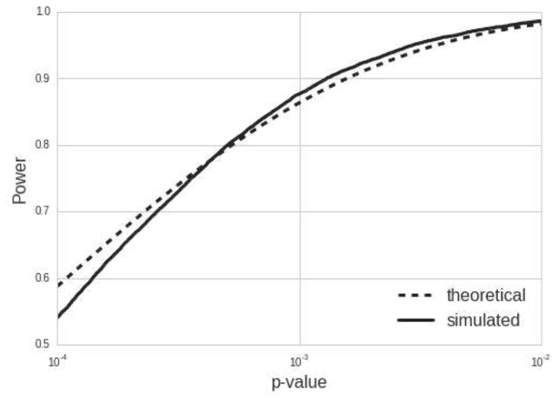
Theoretical power vs. simulated power with scaling factor uncertainty
Table 5 shows the scaling factor variability (CVa) for the selected ROIs, which range from 2 to 8 %. The full distribution of CVa for all the Freesurfer ROIs is shown in Figure 7. To derive the maximum acceptable CVa for 80% power, the theoretical power equation was solved at various subject and site sample sizes with the standardized effect size we detected in our local single center cohort (0.2). The distribution of CVa across all ROIs was plotted adjacent to the power curves (Figure 7) to understand how many ROIs would need to be calibrated for each case. Finally, figures 4, 5, and 6 show the scaling factors from the calibration between two scanners with different sequences at UCSF. Scaling factors derived from the healthy controls (HC) and MS subjects were identical for subcortical gray matter volume (1.05) and very similar for cortical gray matter volume (1, 1.002 for HC, MS) and white matter volume (.967, .975 for HC, MS).
Table 5.
Coefficient of variability (CVa) values for selected ROIs. CVa was defined in equation 14. The ROIs are gray matter volume (GMV), subcortical gray matter volume (scGMV), cortex volume (cVol), cortical white matter volume (cWMV, which does not include cerebellar white matter), and the volumes of the lateral ventricle (LV), amygdala (Amyg), thalamus (Thal), hippocampus (Hipp), caudate (Caud), and finally the estimated total intracranial volume (eTIV)
| CVa | |
|---|---|
| variable | |
| LV (L) | 0.03 |
| LV (R) | 0.03 |
| cWMV | 0.02 |
| cVol | 0.04 |
| scGMV | 0.02 |
| GMV | 0.04 |
| Caud (L) | 0.02 |
| Caud (R) | 0.07 |
| Amyg (R) | 0.09 |
| Amyg (L) | 0.07 |
| Hipp (L) | 0.03 |
| Hipp (R) | 0.03 |
| Thal (L) | 0.05 |
| Thal (R) | 0.05 |
Figure 7.

Shows power curves for 80% power for 2260 – 3000 total subjects, where the false positive rate is 0.002, and the effect size is 0.2. The lowest point of each curve shows the minimum number of sites required for a given number of subjects on the x-axis and the y-axis corresponds to the maximum acceptable coefficient of variability (CVa, defined in 14) for that case. The right-hand side of the chart shows the distribution of CVa values across all sites and all Freesurfer ROIs. When minimizing the total number of sites for a set number of subjects, the maximum allowable CVa is around 5%, meaning that if the CVa is higher than 5% for a particular ROI, the power of the model will fall below 80%. The shaded section on the bottom of the chart called the “Harmonization Zone” which indicates the regions of the graph where the maximum acceptable CVa is below the largest CVa across all freesurfer ROIs (which is the right amygdala at 9%). If site- and subject- level sample sizes fall within the harmonization zone, efforts to harmonize between sites is required to guarantee power for all ROIs.
Figure 4.

Sub-cortical gray matter volume (scGMV) calibration between 2 scanners/sequences at UCSF. The trendline fit shows the slopes (scaling factors) are identical for the healthy control and MS populations
Figure 5.

Cortex gray matter volume (cVol) calibration between 2 scanners/sequences at UCSF. The trendline fit shows the slopes (scaling factors) are very close for the healthy control and MS populations
Figure 6.

White matter volume (WMV) calibration between 2 scanners/sequences at UCSF. The trendline fit shows the slopes (scaling factors) are very close for the healthy control and MS populations
5. Discussion
In this study we proposed a statistical model based on on the physics of MRI volumetric biases using the key assumption that biases between sites are scaled linearly. Variation in scaling factors could explain why a study may estimate different effect sizes based on the pulse sequence used. For example, [38] found significant effects of RF head coils, pulse sequences, and resolution on VBM results. The estimation of scaling factors in our model depends on good scan-rescan reliability. In our study, scan-rescan reliabilities for each scanner were generally > 0.8 for Freesurfer-derived regional volumes. Volumes of cortex, cortical gray, subcortical gray, and cortical white matter parcellation had greater than 90% reliability for all 20 sites. The subcortical regions and estimated total intracranial volume had an average reliability of over 89%, however, some sites had much lower scan-rescan reliability. For example, the thalamus at sites 3 and 16 had test-retest reliabilities between 41 and 63 %. This could be explained by the visual quality control process of the segmented images, which focused on the cortical gray matter segmentation and the initial standard space registration only, due to time restrictions. Visually evaluating all regional segmentations may be unrealistic for a large multisite study. On the other hand, Jovicich and colleagues [39] reported a low within-site ICC of the thalamus across sessions (0.765 ± 0.183) using the same freesurfer cross-sectional pipeline as this study. The poor between-site reliability (61%) of the thalamus is consistent with findings from [40], in which a multisite VBM analysis showed poor consistency in that region. Other segmentation algorithms may be more robust for subcortical regions in particular. Using FSL’s FIRST segmentation algorithm, Cannon and colleagues [1] report a between-site ICC of the thalamus of 0.95, compared to our calibrated between-site ICC of 0.78. FSL’s FIRST algorithm [41] uses a Bayesian model of shape and intensity features to produce a more precise segmentation. Nugent and colleagues reported the reliability of the FIRST algorithm across 3 platforms. Their study of subcortical ROIs found a good scan-rescan reliability of 83%, but lower between-site ICCs ranging from 57% to 93% [42]. The LEAP algorithm proposed by Wolz and colleagues [43] was shown to be extremely reliable with strong ICCs > 0.97 for hippocampal segmentations [14]. Another factor not accounted for in our segmentation results was the effect of partial voluming, which adds uncertainty to tissue volume estimates. In [44], researchers developed a method to more accurately estimate partial volume effects using only T1-weighed images from the ADNI dataset. This approach resulted in higher classification accuracy between Alzheimer’s disease (AD) patients and mild cognitively impaired (MCI) patients from normal controls (NL). Designing optimized pipelines that are robust for each site, scanner make, and metric, is outside the scope of this paper. However, Kim and colleagues have developed a robust technique for tissue classification of heterogeneously acquired data that incorporates iterative bias field correction, registration, and classification [45]. Wang and colleagues developed a method to reduce systematic errors of segmentation algorithms relative to manual segmentations by training a wrapper method that learns spatial patterns of systematic errors [46]. Methods such as those employed by Wang and colleagues may be preferred over standard segmentation pipelines when data acquisition is not standardized. Due to its wide range of acquisition parameters and size of the dataset, our approach could be used to evaluate such generalized pipelines in the future.
The above derivation of power for a multisite study defines hard thresholds for the amount of acceptable scaling factor variability (CVa) using scaled, systematic error from MRI. Many factors contribute to the CVa cut-off, such as the total number of subjects, total number of sites, effect size, and false positive rate. In Figure 7, we show the distribution of experimental CVa values across all Freesurfer aseg ROIs to reference while comparing power curves of various sample sizes. The maximum CVa value is 9% which, with enough subjects and sites, falls well below the maximum acceptable CVa value. However, with the minimum number of subjects and sites, the power curves of figure 7 show that the maximum acceptable CVα must be below 5% for 80% power. If we minimize the total number of subjects to 2260 for the 20 sites in our study, the CVa of the amygdala does not meet this requirement (see table 5). One option to address this is to harmonize protocols, which may reduce CVa values below those estimated from our sites such that they satisfy the maximum CVa requirement. The other option is to recruit more subjects per site. The number of additional subjects needed to overcome a large CVa can be estimated using our power equation. In the case of the parameters defined in figure 7 (a small effect size of 0.2, false positive rate of 0.002), 40 additional subjects beyond the initial 2260 are needed to adequately power the study. This is easily visualized in figure 7: the point on the curve for the initial 2260 subjects over 20 sites lies below the harmonization zone, while that of 2300 total subjects lies above. The number of additional subjects needed to achieve an adequately powered multisite study depends on effect sizes, false positive rates, power requirements, and site-level sample size.
We have validated our scaling factors by demonstrating that a leave-one-out calibration resulted in increased absolute agreement between sites compared to the original, uncalibrated values for 44 out of 46 ROIs studied. Tables 6 and 7 compare these calibrated and original values to the ICC findings of other harmonization efforts. Table 6 compares our between-site ICCs before and after scaling factor calibration to those of [1]. [1] used a cortical pattern matching segmentation algorithm [47] for the cortical ROIs and FSL’s FIRST algorithm for the subcortical ROIs. The between-site ICC for gray matter volume (GMV) for our study was 0.78 while [1] reported an ICC of 0.85. This difference could be explained by the harmonization of scanners in [1]. After using the scaling factors to calibrate GMV, the between-site ICC increased to 0.96, indicating that the estimated CVa of GMV (4%) is an accurate representation of the true between-site bias variability. Scaling calibration of the hippocampus also outperformed the between-site ICC of [1] (0.84 versus 0.79), validating the CVa estimate of 3% for both hemispheres. For the amygdala and caudate volumes, scaling calibration showed improvement to nearly the same value as [1]. The amygdala increased from 0.54 to 0.74 (versus 0.76 in the [1]), and the ICC of the caudate increased from 0.82 to 0.91 (versus 0.92 in the [1]). The CVa of the left and right amygala were the highest in our study, at 7 and 9 percent, respectively. The most extreme asymmetry in the scaling factors was between the left and right caudate (2% and 7%, respectively), which demonstrates regional contrast to noise variation. Even after scaling factor calibration, the between-site ICC produced by our approach varied widely from that of [1] in two ROIs. The between-site ICC of white matter volume (WMV) was very high (0.96 versus 0.774) and that of thalamus volume was very low (.61 versus .95), compared to [1]. This could be due to differences algorithm differences (FIRST vs. Freesurfer). It should also be noted that the scan-rescan reliability of the thalamus was particularly low in some sites, which propagated errors to scaling factor estimates. Therefore, the 5% CVa estimate for the thalamus in both hemispheres may not be reproducible and would need to be recalculated using a different algorithm.
Table 6.
Between-site ICC comparison to the study by [1], where MRI sequences were standardized and subcortical segmentation was performed using FIRST, and cortical segmentation using cortical pattern matching. ICC BW and ICC BW Cal were calculated using our multisite healthy control data, where ICC BW Cal was calculated as the between site ICC of volumes after applying the scaling factor from a leave-one-out calibration. Other than the thalamus (Thal), we found that the between-site ICCs were comparable to [1] for the amygdala (Amyg), caudate (Caud), and even higher for the hippocampus (Hipp), gray matter volume (GMV) and white matter volume (WMV)
| ROI | ICC BW | ICC BW Cal | [1] ICC BW |
|---|---|---|---|
| GMV | .78 | .96 | .854 |
| WMV | .96 | .98 | .774 |
| Thal | .61 | .73 | .95 |
| Hipp | .75 | .84 | .79 |
| Amyg | .56 | .74 | .76 |
| Caud | .82 | .91 | .92 |
Table 7.
Comparing the within-site ICC before and after leave-one-out scaling factor calibration with the cross-sectional freesurfer results of [39], where scanners were standardized, and the average within-site ICC is shown. The within-site ICCs of our study fall within the range of [39], which shows the that sites in this study are as reliable as those in [39].
| ROI | ICC WI | ICC WI Cal | [39] ICC WI Average |
|---|---|---|---|
| LV | 1 | 1 | .998 ± 0.002 |
| Thal | .86 | .84 | 0.765 ± .183 |
| Hipp | .93 | .93 | 0.878 ± .132 |
| Amyg | .89 | .86 | 0.761 ± .134 |
| Caud | .97 | .97 | 0.909 ± 0.092 |
Table 7 shows comparisons of our within-site ICCs to the average within-site ICCs reported by [39]. Similar to our study, scanners were not strictly standardized and the freesurfer cross-sectional algorithm was run. All within site ICCs (both before and after scaling factor calibration) fall within the range described by [39], including the thalamus. Our last attempt to validate this statistical model and accompanying scaling factor estimates was to simulate multisite data using scaling factor estimates and their residual error from the estimate. We found that the power curves align closely, and match when power is at least 80%. We believe that the small deviations from the theoretical model result from scaling factor estimation error and a non-normal scaling factor distribution due to a relatively small sampling of scaling factors (J = 20 sites).
The data acquisition of our study is similar to that of [48], in which the researchers acquired T1-weighted images from 8 consistent human phantoms across 5 sites with non-standardized protocols. These scanners were all 1.5T except for one 1T scanner. [48] calibrated the intensity histograms of the images before segmentation with a calibration factor estimated based on the absolute agreement of volumes to the reference site (ICC). After applying their calibration method, the ICC of the lateral ventricle was ≥ 0.96, which is similar to our pre- and post- calibrated result of 0.97. The ICC for the intensity calibrated gray matter volume in [48] was ≥ 0.84, compared to our calibrated between-site ICC of 0.78 (uncalibrated), and 0.96 (calibrated). Our between-site ICCs for white matter volume (0.96 and 0.98 for the pre- and post- calibrated volumes, respectively) were much higher than those of the intensity calibrated white matter volume in [48] (≥ .78). This could be explained by the fact that our cohort of sites is a consortium studying multiple sclerosis, which is a white matter disease, so there may be a bias toward optimizing scan parameters for white matter. Most importantly, the calibration method of [48] requires re-acquisition of a human phantom cohort at each site for each multisite study. Alternatively, multisite studies employing our approach can use the results of our direct-volume calibration (the estimates of CVa for each ROI) to estimate sample sizes based on our proposed power equation and bias measurements without acquiring their own human phantom dataset to use in calibration.
To our knowledge, this is the first study measuring scaling factors between sites with non-standardized protocols using a single set of subjects, and deriving an equation for power that takes this scaling into account via mixed modeling. This study builds on the work of [31], which investigated the feasibility of pooling retrospective data from three different sites with non-standardized sequences using standard pooling, mixed effects modeling, and fixed effects modeling. [31] found that mixed effects and fixed effects modeling outperformed standard pooling. Our statistical model specifies howMRI bias between sites affects the cross-sectional mixed effects model, so it is limited to powering cross-sectional study designs. Jones and colleagues have derived sample size calculations for longitudinal studies acquired under heterogeneous conditions without the use of calibration subjects [49]. This can be useful for studies measuring longitudinal atrophy over long time periods, during which scanners and protocols may change. For the cross-sectional case, the use of random effects modeling enables us to generalize our results to any protocol with acquisition parameters similar to those described here (primarily MPRAGE). If protocols change drastically compared to our sample of 3D MPRAGE-type protocols, a small set of healthy controls should be scanned before and after any major software, hardware, or protocol change so that the resulting scaling factors can be compared to the distribution of scaling factors (CVa) reported in this study. A large CVa can severely impact the power of a multisite study, so it is important not to generalize the results in this study to non-MPRAGE sequences without validation. Potentially, new 3D-printed brain-shaped phantoms with similar regional contrast to noise ratios as human brains may become an excellent option for estimating CVa.
A limitation of our model is the assumption of independence between the unobserved effect (DU,j) at a particular site, j, with the scaling factor of that site (aj). This assumption does not hold if patients with more severe disease have tissue with different properties that, when scanned, shows different regional contrast than that of healthy controls. As shown in the Appendix, the calculation of the unconditional variance of the observed estimate (equation 7) can get quite complicated. We addressed this issue for multiple sclerosis patients by showing that the scaling factors from healthy controls are very similar to those derived from an MS population. The largest difference in scaling factors between healthy controls and multiple sclerosis patients was in white matter volume, where aMS = 0.967 and aHC = 0.975. A two-sample T test between the scaling factors produced a p-value of 0.88, showing that we could not detect a significant difference between scaling factors of HC and MS. This part of the study was limited in that we only scanned MS patients at two scanners, while the healthy controls were scanned at 20, so we could not estimate a patient-derived CVa (the direct input to the power equation). However, the similarity between scaling factors for the subcortical gray matter, cortical gray matter, and white matter volumes between the MS and HC populations suggests that, given careful editing of volumes in the disease population, the independence assumption holds for MS. We recommend that researchers studying other diseases validate our approach by scanning healthy controls and patients before and after an upgrade or sequence change to test the validity of the independence assumption.
Even though we did not standardize the protocols and scanners within this study, the consortium is unbalanced in that there are 16 3T scanners, 11 of which are Siemens. Of the Siemens 3T scanners, there is little variability in TR, TE, and TI, however, there is more variance in the use of parallel imaging, the number of channels in the head coil (12, 20 or 32), and the field of view. Similar to the findings of [50], we could not detect differences in scan-rescan reliability between field strengths. Wolz and colleagues could not detect differences in scan-rescan reliabilities of the hippocampus volumes estimated by the LEAP algorithm, but they detected a small bias between field strengths. They found that the hippocampus volumes measured from the 3T ADNI scanners were 1.17 % larger than those measured from the 1.5T [14]. A two-sample T-test with unequal variances was run between the scaling factors of the 1.5T versus 3T scanners. This test could not detect differences in any ROI except for the left- and right-amydgala. We found that the scaling factors were lower for the 1.5T scanners than for the 3T scanners (0.9 versus 1.02), suggesting that the amygdala volume estimates from the 1.5T were larger than those of the 3T. It should be noted that this interpretation is limited due to the small sample size of 1.5T scanners in this consortium.
Another limitation of this study is that we were under-powered to accurately estimate both the scaling and intercept for a linear model between two sites, and that we did not take the intercept into account when deriving power. We excluded the intercept from our analysis for two reasons: (1) we believe that the nature of systematic error from MRI segmentation is not additive, meaning that offsets in metrics between sites for different subjects is scaled with ROI size instead of a constant additive factor and (2) the model becomes more complicated if site-level effects are both multiplicative and additive. The other limitation of this study is that we assumed that subjects across all sites will come from the same population, and that stratification occurs solely from systematic errors within each site. In reality, sites may recruit from different populations and the true disease effect will vary even more. For example, in a comparison study between the matched ADNI cohort and a matched Mayo Clinic Study of Aging cohort, researchers found different rates of hippocampal atrophy even though no differences in hippocampal volume was detected [51]. This could be attributed to sampling from two different populations. This added site-level variability requires a larger site-level sample size, for an example of modeling this, see [52].
In this study, we reported reliability using both between-site ICC and CVa because these two metrics have complementary advantages. ICC depends on the true subject-level variability studied. Since we scanned healthy controls, our variance component estimates of subject variability may be lower than that of our target population (patients with multiple sclerosis related atrophy). As a result, ICCs may be lower than expected in MS based on the results of healthy controls. We tried to address this issue by scanning subjects in a large age range, capturing the variability in gray and white matter volume due to atrophy from aging. On the other hand, CVa is invariant to true subject variability, but is limited by the accuracy of between-site scaling estimates. Both between-site ICC and CVa should be reported when evaluating multisite reliability datasets to understand a given algorithm’s ability to differentiate between subjects (via the ICC) and the magnitude of systemic error between sites (via the CVa), which could be corrected using harmonization.
6. Conclusion
When planning a multisite study, there is an emphasis on acquiring data from more sites because the estimated effect sizes from each site are sampled from a distribution and averaged. Understanding how much of the variance in the distribution is due to scanner noise as opposed to population heterogeneity is an important part of powering a study. For the purposes of this study, we estimated the effect size variability of Freesurfer-derived regional volumes, but this framework could be generalized to any T1-weighted segmentation algorithm, and any modality for which systematic errors are scaled. Scaling factor calibration of metrics resulted in higher absolute agreement of metrics between sites, which showed that the scaling factor variabilities for the ROIs in this study were accurate. The equation for power we outlined in this study along with our measurements of variability between sites should help researchers undestand the trade-off between protocol harmonization and sample size optimization, along with the choice of outcome metrics. Our statistical model and bias measurements enables collaboration between research institutions and hospitals when hardware and software adaptation are not feasible. We provide a comprehensive framework for assessing and making informed quantitative decisions for MRI facility inclusion, pipeline and metric optimization, and study power.
Supplementary Material
Table 2.
Top: Acquisition parameters for the 3T Philips and GE scanners. Ph = Philips, GE= General Electric. Bottom: Test-retest reliabilities for selected ROIs, processed by Freesurfer. The ROIs are gray matter volume (GMV), subcortical gray matter volume (scGMV), cortex volume (cVol), cortical white matter volume (cWMV), and the volumes of the lateral ventricle (LV), amygdala (Amyg), thalamus (Thal), hippocampus (Hipp), caudate (Caud), and finally the estimated total intracranial volume (eTIV). Test-retest reliability is computed as within-site ICC(1,1)
| 5 | 6 | 7 | 8 | 9 | |
|---|---|---|---|---|---|
| TR (ms) | 8.21 | 7.80 | 9 | 8.21 | 6.99 |
| TE (ms) | 3.22 | 2.90 | 4.00 | 3.81 | 3.16 |
| Strength (T) | 3 | 3 | 3 | 3 | 3 |
| TI (ms) | 450 | 450 | 1000 | 1016.30 | 900 |
| Flip Angle (°) | 12 | 12 | 8 | 8 | 9 |
| Make | GE | GE | Ph | Ph | Ph |
| Voxel Size (mm) | .94×.94×1 | 1×1×1.2 | 1×1×1 | 1×1×1 | 1×1×1 |
| Distortion Correction | N | Y | Y | Y | Y |
| Parallel Imaging | 2 | 2 | 3 | 2 | - |
| FOV (mm) | 240×240×172 | 256×256×166 | 240×240×170 | 240×240×160 | 256×256×204 |
| Read Out Direction | HF | FH | AP | FH | FH |
| Head coil # channels | 8 | 8 | 16 | 32 | 8 |
| Model | MR750 | Signa HDxt | Achieva | Achieva TX | Intera |
| OS | DV24 | HD23.0 V01 1210a | 3.2.3.2 | 5.1.7 | 3.2.3 |
| Acq. Time (min) | 5:02 | 7:11 | 05:55 | 05:38 | 08:30:00 |
| orientation | sag | sag | sag | sag | sag |
| # scans | 24/24 | 24/24 | 24/24 | 24/24 | 21/22 |
|
| |||||
| Amyg (L) | .67 | .89 | .66 | .85 | 0.97 |
| Amyg (R) | .88 | .79 | .91 | .94 | 0.94 |
| Caud (L) | .96 | .98 | .98 | .97 | 0.98 |
| Caud (R) | .95 | .96 | .98 | .93 | 0.96 |
| GMV | 1 | .99 | .99 | .98 | 0.99 |
| Hipp (L) | .51 | .97 | .83 | .90 | 0.99 |
| Hipp (R) | .95 | .96 | .93 | .96 | 0.99 |
| Thal (L) | .97 | .81 | .94 | .80 | 0.88 |
| Thal (R) | .70 | .87 | .96 | .96 | 0.97 |
| cVol | .99 | .99 | .98 | .98 | 0.99 |
| cWMV | 1 | .99 | 1 | 1 | 1.00 |
| eTIV | 1 | 1 | 1 | .92 | 0.99 |
| scGMV | .98 | .99 | .96 | .98 | 0.99 |
Table 3.
Top: Acquisition parameters for the 3T Siemens (Si) Skyra and Prisma scanners. Bottom: Test-retest reliabilities for selected ROIs, processed by Freesurfer. The ROIs are gray matter volume (GMV), subcortical gray matter volume (scGMV), cortex volume (cVol), cortical white matter volume (cWMV), and the volumes of the lateral ventricle (LV), amygdala (Amyg), thalamus (Thal), hippocampus (Hipp), caudate (Caud), and finally the estimated total intracranial volume (eTIV). Test-retest reliability is computed as within-site ICC(1,1)
| 10 | 11 | 12 | 13 | 14 | 15 | |
|---|---|---|---|---|---|---|
| TR (ms) | 2300 | 2300 | 2300 | 2300 | 2300 | 2000 |
| TE (ms) | 2.96 | 2.98 | 2.98 | 2.96 | 2.96 | 3.22 |
| Strength (T) | 3 | 3 | 3 | 3 | 3 | 3 |
| TI (ms) | 900 | 900 | 900 | 900 | 900 | 900 |
| Flip Angle (°) | 9 | 9 | 9 | 9 | 9 | 8 |
| Make | Si | Si | Si | Si | Si | Si |
| Voxel Size (mm) | 1×1×1 | 1×1×1.1 | 1×1×1 | 1×1×1 | 1×1×1 | 1×1×1 |
| Distortion Correction | Y | N | Y | Y | Y | N |
| Parallel Imaging | 2 | - | 2 | 2 | 2 | 2 |
| FOV (mm) | 256×256×176 | 240×256×176 | 240×256×176 | 240×276×156 | 256×256×176 | 256×208×160 |
| Read Out Direction | HF | RL | HF | HF | HF | RL |
| Head coil # channels | 20 | 32 | 20 | 20 | 20 | 32 |
| Model | Prisma | Prisma fit | Skyra | Skyra | Skyra | Skyra |
| OS | D13D | VD13D | VD13 | VD13 | VD13C | VD13 |
| Acq. Time (min) | 05:09 | 07:46 | 05:12 | 05:12 | 05:09 | 04:56 |
| orientation | sag | sag | sag | sag | sag | ax |
| # scans | 22/22 | 24/24 | 25/25 | 23/24 | 23/24 | 22/22 |
|
| ||||||
| Amyg (L) | .83 | .89 | .80 | .85 | .98 | .89 |
| Amyg (R) | .94 | .92 | .93 | .85 | .93 | .84 |
| Caud (L) | .99 | .99 | .98 | .99 | .98 | .98 |
| Caud (R) | .99 | .96 | .95 | .95 | .98 | .97 |
| GMV | .99 | .98 | .99 | 1 | .99 | .97 |
| Hipp (L) | .94 | .98 | .99 | .95 | .97 | .98 |
| Hipp (R) | .91 | .94 | .97 | .98 | .95 | .96 |
| Thal (L) | .92 | .87 | .87 | .76 | .91 | .89 |
| Thal (R) | .74 | .93 | .80 | .91 | .93 | .89 |
| cVol | .99 | .98 | .98 | 1 | .99 | .96 |
| cWMV | 1 | 1 | 1 | 1 | 1 | .97 |
| eTIV | 1 | 1 | 1 | 1 | 1 | .97 |
| scGMV | .98 | .99 | .98 | .98 | .99 | .99 |
Highlights.
We hypothesize that biases of MRI regional volumes between scanners are scaled based on regional constrast and gradient distortions
Given this scaling property, we define a statistical model and provide a power equation
We measured the variability between regional volumes estimated from 12 subjects scanned in 20 nonstandardized scanners
Our statistical model combined with our bias measurements allows researchers to optimize sample sizes rather than harmonize protocols for future multisite MRI studies on regional volumes.
Acknowledgments
We thank the study participants, MR technicians, and acknowledge Stephane Lehéricy, Eric Bardinet, Frédéric Humbert and Antoine Burgos from the ICM IRM facility (CENIR) and the CIC Pitié-Salpêtrière for their expertise. Funding was provided by R01 NS049477. Additional support was provided by ICM F-75013 Paris, INSERM and IHU-A-ICM (ANR-10-IAIHU-06). BD is a Clinical Investigator of the Research Foundation Flanders (FWO-Vlaanderen). AG and BD are supported by the Research Fund KU Leuven (OT/11/087) and the Research Foundation Flanders (G0A1313N). MRI acquisitions in Hospital Clinic of Barcelona were funded by a “Proyecto de Investigación en Salut” grant (PI15/00587. PIs Albert Saiz and Sara Llufriu) from the Instituto de Salud Carlos III.
10. Appendix
10.1. Variance of a Product of Random Variables
The proof for this is found in Introduction to the Theory of Statistics (1974) by Mood, Graybill and Boes [53], section 2.3, Theorem 3:
Let X and Y be two random variables where var[XY] exists, then
| (17) |
which can be obtained by computing E[XY] and E[(XY)2] when XY is expressed as
| (18) |
If X and Y are independent, then E[XY] = μXμY, the covariance terms are 0, and
| (19) |
and
| (20) |
| (21) |
Which gives
| (22) |
10.2. Maximum Likelihood
Note that the estimator defined in 9 is a maximum likelihood estimator under the condition of equal unexplained variance at each site and an equal number of subjects at each site. In the case with different number of subjects at each site, the maximum likelihood estimator for the disease effect, β̂10, is not the average of the site-level coefficients, but instead is the average weighted by the inverse error variance. This is a common method to run meta-analyses, for example, see [52, 6]. To show this, we follow the procedure from [52], and define the likelihood of the alternate hypotheses as
| (23) |
for a non-zero μ and Vj defined as the unscaled error variance on . The maximum likelihood estimator μ̂ is found by taking the derivative of the log of (23), setting it equal to 0, and solving for μ,
| (24) |
which shows that the inverse variance weighted average is the maximum likelihood estimator for the overall treatment effect. If we assume that the unexplained variance (σ0) is the same across all sites, which is a valid assumption if subjects are from the same population, the estimate can be expressed as
| (25) |
where is the total number of subjects in the study. The variance of the estimate is
| (26) |
and it follows that the noncentrality parameter is
| (27) |
which should be used for a more accurate power analysis if the specific number of subjects per site and the site’s scaling factors are known.
Footnotes
Publisher's Disclaimer: This is a PDF file of an unedited manuscript that has been accepted for publication. As a service to our customers we are providing this early version of the manuscript. The manuscript will undergo copyediting, typesetting, and review of the resulting proof before it is published in its final citable form. Please note that during the production process errors may be discovered which could affect the content, and all legal disclaimers that apply to the journal pertain.
References
- 1.Cannon TD, Cadenhead K, Cornblatt B, Woods SW, Addington J, Walker E, Seidman LJ, Perkins D, Tsuang M, McGlashan T, et al. Reliability of neuroanatomical measurements in a multisite longitudinal study of youth at risk for psychosis. Human Brain Mapping. 2014;35(5):2424–2434. doi: 10.1002/hbm.22338. URL http://dx.doi.org/10.1002/hbm.22338. [DOI] [PMC free article] [PubMed] [Google Scholar]
- 2.Ewers M, Teipel S, Dietrich O, Schönberg S, Jessen F, Heun R, Scheltens P, van de Pol L, Freymann N, Moeller H-J, et al. Multicenter assessment of reliability of cranial MRI. Neurobiology of Aging. 2006;27(8):1051–1059. doi: 10.1016/j.neurobiolaging.2005.05.032. [DOI] [PubMed] [Google Scholar]
- 3.Jovicich J, Czanner S, Greve D, Haley E, van der Kouwe A, Gollub R, Kennedy D, Schmitt F, Brown G, MacFall J, Fischl B, Dale A. Reliability in multi-site structural MRI studies: Effects of gradient non-linearity correction on phantom and human data. Neuro Image. 2006;30(2):436– 443. doi: 10.1016/j.neuroimage.2005.09.046. URL http://www.sciencedirect.com/science/article/B6WNP-4HM7S0B-2/2/4fa5ff26cad90ba3c9ed12b7e12ce3b6. [DOI] [PubMed] [Google Scholar]
- 4.Boccardi M, Bocchetta M, Ganzola R, Robitaille N, Redolfi A, Duchesne S, Jack C, Jr, Frisoni G. EADC-ADNI Working Group on The Harmonized Protocol for Hippocampal Volumetry and for the Alzheimer’s Disease Neuroimaging Initiative: Operationalizing protocol differences for EADC-ADNI manual hippocampal segmentation. Alzheimers Dement [Google Scholar]
- 5.Weiner MW, Veitch DP, Aisen PS, Beckett LA, Cairns NJ, Green RC, Harvey D, Jack CR, Jagust W, Liu E, et al. The Alzheimer’s Disease Neuroimaging Initiative: A review of papers published since its inception. Alzheimer’s & Dementia. 2012;8(1):S1–S68. doi: 10.1016/j.jalz.2011.09.172. [DOI] [PMC free article] [PubMed] [Google Scholar]
- 6.Thompson PM, Stein JL, Medland SE, Hibar DP, Vasquez AA, Renteria ME, Toro R, Jahanshad N, Schumann G, Franke B, et al. The ENIGMA Consortium: large-scale collaborative analyses of neuroimaging and genetic data. Brain imaging and behavior. 2014;8(2):153–182. doi: 10.1007/s11682-013-9269-5. [DOI] [PMC free article] [PubMed] [Google Scholar]
- 7.Fonov VS, Janke A, Caramanos Z, Arnold DL, Narayanan S, Pike GB, Collins DL. Medical Imaging and Augmented Reality. Springer; 2010. Improved precision in the measurement of longitudinal global and regional volumetric changes via a novel MRI gradient distortion characterization and correction technique; pp. 324–333. [Google Scholar]
- 8.Gunter JL, Bernstein MA, Borowski BJ, Ward CP, Britson PJ, Felmlee JP, Schuff N, Weiner M, Jack CR. Measurement of MRI scanner performance with the ADNI phantom. Medical physics. 2009;36(6):2193–2205. doi: 10.1118/1.3116776. [DOI] [PMC free article] [PubMed] [Google Scholar]
- 9.Caramanos Z, Fonov VS, Francis SJ, Narayanan S, Pike GB, Collins DL, Arnold DL. Gradient distortions in MRI: characterizing and correcting for their effects on SIENA-generated measures of brain volume change. Neuro Image. 2010;49(2):1601–1611. doi: 10.1016/j.neuroimage.2009.08.008. [DOI] [PubMed] [Google Scholar]
- 10.Droby A, Lukas C, Schänzer A, Spiwoks-Becker I, Giorgio A, Gold R, De Stefano N, Kugel H, Deppe M, Wiendl H, et al. A human post-mortem brain model for the standardization of multi-centre MRI studies. Neuro Image. 2015;110:11–21. doi: 10.1016/j.neuroimage.2015.01.028. [DOI] [PubMed] [Google Scholar]
- 11.Tardif CL, Collins DL, Pike GB. Regional impact of field strength on voxel-based morphometry results. Human brain mapping. 2010;31(7):943–957. doi: 10.1002/hbm.20908. [DOI] [PMC free article] [PubMed] [Google Scholar]
- 12.Tardif CL, Collins DL, Pike GB. Sensitivity of voxel-based morphometry analysis to choice of imaging protocol at 3 T. Neuroimage. 2009;44(3):827–838. doi: 10.1016/j.neuroimage.2008.09.053. [DOI] [PubMed] [Google Scholar]
- 13.Brunton S, Gunasinghe C, Jones N, Kempton M, Westman E, Simmons A. A voxel-based morphometry comparison of the 3.0T ADNI-1 and ADNI-2 MPRAGE protocols. Alzheimer’s & Dementia. 9(4):2013, P581. doi: 10.1016/j.jalz.2013.05.1154. URL http://dx.doi.org/10.1016/j.jalz.2013.05.1154. [DOI] [PMC free article] [PubMed] [Google Scholar]
- 14.Wolz R, Schwarz AJ, Yu P, Cole PE, Rueckert D, Jack CR, Raunig D, Hill D. Robustness of automated hippocampal volumetry across magnetic resonance field strengths and repeat images. Alzheimer’s & Dementia. 2014;10(4):430–438.e2. doi: 10.1016/j.jalz.2013.09.014. URL http://dx.doi.org/10.1016/j.jalz.2013.09.014. [DOI] [PubMed] [Google Scholar]
- 15.Filippi M, Paty D, Kappos L, Barkhof F, Compston D, Thompson A, Zhao G, Wiles C, Mc-Donald W, Miller D. Correlations between changes in disability and T2-weighted brain MRI activity in multiple sclerosis A follow-up study. Neurology. 1995;45(2):255–260. doi: 10.1212/wnl.45.2.255. [DOI] [PubMed] [Google Scholar]
- 16.Furby J, Hayton T, Altmann D, Brenner R, Chataway J, Smith K, Miller D, Kapoor R. A longitudinal study of MRI-detected atrophy in secondary progressive multiple sclerosis. Journal of neurology. 2010;257(9):1508–1516. doi: 10.1007/s00415-010-5563-y. [DOI] [PubMed] [Google Scholar]
- 17.Kappos L, Moeri D, Radue EW, Schoetzau A, Schweikert K, Barkhof F, Miller D, Guttmann CR, Weiner HL, Gasperini C, et al. Predictive value of gadolinium-enhanced magnetic resonance imaging for relapse rate and changes in disability or impairment in multiple sclerosis: a meta-analysis. The Lancet. 1999;353(9157):964–969. doi: 10.1016/s0140-6736(98)03053-0. [DOI] [PubMed] [Google Scholar]
- 18.Horakova D, Kalincik T, Dusankova JB, Dolezal O. Clinical correlates of grey matter pathology in multiple sclerosis. BMC neurology. 2012;12(1):10. doi: 10.1186/1471-2377-12-10. [DOI] [PMC free article] [PubMed] [Google Scholar]
- 19.Sanfilipo MP, Benedict RH, Weinstock-Guttman B, Bakshi R. Gray and white matter brain atrophy and neuropsychological impairment in multiple sclerosis. Neurology. 2006;66(5):685–692. doi: 10.1212/01.wnl.0000201238.93586.d9. [DOI] [PubMed] [Google Scholar]
- 20.Cifelli A, Arridge M, Jezzard P, Esiri MM, Palace J, Matthews PM. Thalamic neurodegeneration in multiple sclerosis. Annals of neurology. 2002;52(5):650–653. doi: 10.1002/ana.10326. [DOI] [PubMed] [Google Scholar]
- 21.Zivadinov R, Bergsland N, Dolezal O, Hussein S, Seidl Z, Dwyer M, Vaneckova M, Krasensky J, Potts J, Kalincik T, et al. Evolution of cortical and thalamus atrophy and disability progression in early relapsing-remitting MS during 5 years. American Journal of Neuroradiology. 2013;34(10):1931–1939. doi: 10.3174/ajnr.A3503. [DOI] [PMC free article] [PubMed] [Google Scholar]
- 22.Houtchens M, Benedict R, Killiany R, Sharma J, Jaisani Z, Singh B, Weinstock-Guttman B, Guttmann C, Bakshi R. Thalamic atrophy and cognition in multiple sclerosis. Neurology. 2007;69(12):1213–1223. doi: 10.1212/01.wnl.0000276992.17011.b5. [DOI] [PubMed] [Google Scholar]
- 23.Wylezinska M, Cifelli A, Jezzard P, Palace J, Alecci M, Matthews P. Thalamic neurodegeneration in relapsing-remitting multiple sclerosis. Neurology. 2003;60(12):1949–1954. doi: 10.1212/01.wnl.0000069464.22267.95. [DOI] [PubMed] [Google Scholar]
- 24.Bermel RA, Innus MD, Tjoa CW, Bakshi R. Selective caudate atrophy in multiple sclerosis: a 3D MRI parcellation study. Neuroreport. 2003;14(3):335–339. doi: 10.1097/00001756-200303030-00008. [DOI] [PubMed] [Google Scholar]
- 25.Tao G, Datta S, He R, Nelson F, Wolinsky JS, Narayana PA. Deep gray matter atrophy in multiple sclerosis: a tensor based morphometry. Journal of the neurological sciences. 2009;282(1):39–46. doi: 10.1016/j.jns.2008.12.035. [DOI] [PMC free article] [PubMed] [Google Scholar]
- 26.Fisher E, Lee J-C, Nakamura K, Rudick RA. Gray matter atrophy in multiple sclerosis: a longitudinal study. Annals of neurology. 2008;64(3):255–265. doi: 10.1002/ana.21436. [DOI] [PubMed] [Google Scholar]
- 27.Fisniku LK, Chard DT, Jackson JS, Anderson VM, Altmann DR, Miszkiel KA, Thompson AJ, Miller DH. Gray matter atrophy is related to long-term disability in multiple sclerosis. Annals of neurology. 2008;64(3):247–254. doi: 10.1002/ana.21423. [DOI] [PubMed] [Google Scholar]
- 28.Dalton CM, Chard DT, Davies GR, Miszkiel KA, Altmann DR, Fernando K, Plant GT, Thompson AJ, Miller DH. Early development of multiple sclerosis is associated with progressive grey matter atrophy in patients presenting with clinically isolated syndromes. Brain. 2004;127(5):1101–1107. doi: 10.1093/brain/awh126. [DOI] [PubMed] [Google Scholar]
- 29.Giorgio A, Battaglini M, Smith SM, De Stefano N. Brain atrophy assessment in multiple sclerosis: importance and limitations. Neuroimaging clinics of North America. 2008;18(4):675–686. doi: 10.1016/j.nic.2008.06.007. [DOI] [PubMed] [Google Scholar]
- 30.Garson GD. Fundamentals of hierarchical linear and multilevel modeling, Hierarchical linear modeling: guide and applications. Sage Publications Inc; 2013. pp. 3–25. [Google Scholar]
- 31.Fennema-Notestine C, Gamst AC, Quinn BT, Pacheco J, Jernigan TL, Thal L, Buckner R, Killiany R, Blacker D, Dale AM, et al. Feasibility of multi-site clinical structural neuroimaging studies of aging using legacy data. Neuroinformatics. 2007;5(4):235–245. doi: 10.1007/s12021-007-9003-9. [DOI] [PubMed] [Google Scholar]
- 32.Raudenbush SW, Liu X. Statistical power and optimal design for multisite randomized trials. Psychological methods. 2000;5(2):199–213. doi: 10.1037/1082-989x.5.2.199. URL http://view.ncbi.nlm.nih.gov/pubmed/10937329. [DOI] [PubMed] [Google Scholar]
- 33.Fischl B, Salat DH, Busa E, Albert M, Dieterich M, Haselgrove C, van der Kouwe A, Killiany R, Kennedy D, Klaveness S, Montillo A, Makris N, Rosen B, Dale AM. Whole brain segmentation: automated labeling of neuroanatomical structures in the human brain. Neuron. 2002;33:341–355. doi: 10.1016/s0896-6273(02)00569-x. [DOI] [PubMed] [Google Scholar]
- 34.Buckner RL, Head D, Parker J, Fotenos AF, Marcus D, Morris JC, Snyder AZ. A unified approach for morphometric and functional data analysis in young, old, and demented adults using automated atlas-based head size normalization: reliability and validation against manual measurement of total intracranial volume. Neuroimage. 2004;23(2):724–738. doi: 10.1016/j.neuroimage.2004.06.018. [DOI] [PubMed] [Google Scholar]
- 35.Friedman L, Stern H, Brown GG, Mathalon DH, Turner J, Glover GH, Gollub RL, Lauriello J, Lim KO, Cannon T, et al. Test–retest and between-site reliability in a multicenter fMRI study. Human brain mapping. 2008;29(8):958–972. doi: 10.1002/hbm.20440. [DOI] [PMC free article] [PubMed] [Google Scholar]
- 36.Revelle W. psych: Procedures for Psychological, Psychometric, and Personality Research, Northwestern University, Evanston, Illinois. r package version 1.5.8. 2015 URL http://CRAN.R-project.org/package=psych.
- 37.Kurtzke JF. Rating neurologic impairment in multiple sclerosis: An expanded disability status scale (EDSS) Neurology. 1983;33(11):1444–1444. doi: 10.1212/wnl.33.11.1444. URL http://dx.doi.org/10.1212/wnl.33.11.1444. [DOI] [PubMed] [Google Scholar]
- 38.Streitbürger D-P, Pampel A, Krueger G, Lepsien J, Schroeter ML, Mueller K, Möller HE. Impact of image acquisition on voxel-based-morphometry investigations of age-related structural brain changes. Neuroimage. 2014;87:170–182. doi: 10.1016/j.neuroimage.2013.10.051. [DOI] [PubMed] [Google Scholar]
- 39.Jovicich J, Marizzoni M, Sala-Llonch R, Bosch B, Bartrés-Faz D, Arnold J, Benninghoff J, Wiltfang J, Roccatagliata L, Nobili F, et al. Brain morphometry reproducibility in multi-center 3T MRI studies: a comparison of cross-sectional and longitudinal segmentations. Neuroimage. 2013;83:472–484. doi: 10.1016/j.neuroimage.2013.05.007. [DOI] [PubMed] [Google Scholar]
- 40.Schnack HG, van Haren NE, Brouwer RM, van Baal GCM, Picchioni M, Weisbrod M, Sauer H, Cannon TD, Huttunen M, Lepage C, et al. Mapping reliability in multicenter MRI: Voxel-based morphometry and cortical thickness. Human Brain Mapping. 2010;31(12):1967–1982. doi: 10.1002/hbm.20991. [DOI] [PMC free article] [PubMed] [Google Scholar]
- 41.Patenaude B, Smith SM, Kennedy DN, Jenkinson M. A Bayesian model of shape and appearance for subcortical brain segmentation. Neuroimage. 2011;56(3):907–922. doi: 10.1016/j.neuroimage.2011.02.046. [DOI] [PMC free article] [PubMed] [Google Scholar]
- 42.Nugent AC, Luckenbaugh DA, Wood SE, Bogers W, Zarate CA, Drevets WC. Automated subcortical segmentation using FIRST: Test–retest reliability, interscanner reliability, and comparison to manual segmentation. Human brain mapping. 2013;34(9):2313–2329. doi: 10.1002/hbm.22068. [DOI] [PMC free article] [PubMed] [Google Scholar]
- 43.Wolz R, Aljabar P, Hajnal JV, Hammers A, Rueckert D. LEAP: Learning embeddings for atlas propagation. Neuro Image. 2010;49(2):1316–1325. doi: 10.1016/j.neuroimage.2009.09.069. URL http://dx.doi.org/10.1016/j.neuroimage.2009.09.069. [DOI] [PMC free article] [PubMed] [Google Scholar]
- 44.Roche A, Forbes F. Medical Image Computing and Computer-Assisted Intervention – MICCAI 2014. Springer Science + Business Media; 2014. Partial Volume Estimation in Brain MRI Revisited; pp. 771–778. URL http://dx.doi.org/10.1007/978-3-319-10404-1_96. [DOI] [PubMed] [Google Scholar]
- 45.Kim EY, Johnson HJ. Robust Multi-site MR Data Processing: Iterative Optimization of Bias Correction, Tissue Classification, and Registration. Frontiers in Neuroinformatics. 7(29) doi: 10.3389/fninf.2013.00029. URL http://www.frontiersin.org/neuroinformatics/10.3389/fninf.2013.00029/abstract. [DOI] [PMC free article] [PubMed] [Google Scholar]
- 46.Wang H, Das SR, Suh JW, Altinay M, Pluta J, Craige C, Avants B, Yushkevich PA. A learning-based wrapper method to correct systematic errors in automatic image segmentation: Consistently improved performance in hippocampus, cortex and brain segmentation. Neuro Image. 2011;55(3):968– 985. doi: 10.1016/j.neuroimage.2011.01.006. doi: http://dx.doi.org/10.1016/j.neuroimage.2011.01.006. URL http://www.sciencedirect.com/science/article/pii/S1053811911000243. [DOI] [PMC free article] [PubMed] [Google Scholar]
- 47.Thompson PM, Mega MS, Vidal C, Rapoport JL, Toga AW. Information Processing in Medical Imaging. Springer; 2001. Detecting Sisease-Specific Patterns of Brain Structure Using Cortical Pattern Matching and a Population-Based Probabilistic Brain Atlas; pp. 488–501. [DOI] [PMC free article] [PubMed] [Google Scholar]
- 48.Schnack HG, van Haren NE, Pol HEH, Picchioni M, Weisbrod M, Sauer H, Cannon T, Huttunen M, Murray R, Kahn RS. Reliability of brain volumes from multicenter MRI acquisition: A calibration study. Human Brain Mapping. 2004;22(4):312–320. doi: 10.1002/hbm.20040. URL http://dx.doi.org/10.1002/hbm.20040. [DOI] [PMC free article] [PubMed] [Google Scholar]
- 49.Jones BC, Nair G, Shea CD, Crainiceanu CM, Cortese IC, Reich DS. Quantification of multiple-sclerosis-related brain atrophy in two heterogeneous MRI datasets using mixed-effects modeling. Neuro Image: Clinical. 2013;3:171–179. doi: 10.1016/j.nicl.2013.08.001. [DOI] [PMC free article] [PubMed] [Google Scholar]
- 50.Jovicich J, Czanner S, Han X, Salat D, van der Kouwe A, Quinn B, Pacheco J, Albert M, Killiany R, Blacker D. MRI-derived measurements of human subcortical ventricular and intracranial brain volumes: Reliability effects of scan sessions, acquisition sequences, data analyses, scanner upgrade, scanner vendors and field strengths. Neuro Image. 2009;46(1):177–192. doi: 10.1016/j.neuroimage.2009.02.010. URL http://dx.doi.org/10.1016/j.neuroimage.2009.02.010. [DOI] [PMC free article] [PubMed] [Google Scholar]
- 51.Whitwell JL. Comparison of Imaging Biomarkers in the Alzheimer Disease Neuroimaging Initiative and the Mayo Clinic Study of Aging. Arch Neurol. 2012;69(5):614. doi: 10.1001/archneurol.2011.3029. URL http://dx.doi.org/10.1001/archneurol.2011.3029. [DOI] [PMC free article] [PubMed] [Google Scholar]
- 52.Han B, Eskin E. Random-effects model aimed at discovering associations in meta-analysis of genome-wide association studies. The American Journal of Human Genetics. 2011;88(5):586–598. doi: 10.1016/j.ajhg.2011.04.014. [DOI] [PMC free article] [PubMed] [Google Scholar]
- 53.Boes DC, Graybill F, Mood A. Introduction to the Theory of Statistics. Series in probabili [Google Scholar]
Associated Data
This section collects any data citations, data availability statements, or supplementary materials included in this article.