

Abstract
New treatments for organic aerosol (OA) formation have been added to a modified version of the CESM/CAM5 model (CESM‐NCSU). These treatments include a volatility basis set treatment for the simulation of primary and secondary organic aerosols (SOAs), a simplified treatment for organic aerosol (OA) formation from glyoxal, and a parameterization representing the impact of new particle formation (NPF) of organic gases and sulfuric acid. With the inclusion of these new treatments, the concentration of oxygenated organic aerosol increases by 0.33 µg m−3 and that of primary organic aerosol (POA) decreases by 0.22 µg m−3 on global average. The decrease in POA leads to a reduction in the OA direct effect, while the increased OOA increases the OA indirect effects. Simulations with the new OA treatments show considerable improvement in simulated SOA, oxygenated organic aerosol (OOA), organic carbon (OC), total carbon (TC), and total organic aerosol (TOA), but degradation in the performance of HOA. In simulations of the current climate period, despite some deviations from observations, CESM‐NCSU with the new OA treatments significantly improves the magnitude, spatial pattern, seasonal pattern of OC and TC, as well as, the speciation of TOA between POA and OOA. Sensitivity analysis reveals that the inclusion of the organic NPF treatment impacts the OA indirect effects by enhancing cloud properties. The simulated OA level and its impact on the climate system are most sensitive to choices in the enthalpy of vaporization and wet deposition of SVOCs, indicating that accurate representations of these parameters are critical for accurate OA‐climate simulations.
Keywords: CESM/CAM5, secondary organic aerosol, volatility basis set, organic new particle formation, aerosol indirect effects, earth system modeling
Key Points
VBS and other OA updates significantly improve OA model performance
OA‐climate interactions are the most sensitive to enthalpy of vaporization and semivolatile organic compounds wet deposition
The updated CESM‐NCSU OA treatments reasonably simulate OA in the current climate
1. Introduction
Organic aerosol (OA) comprises a significant portion (18–70%) of submicron aerosol [Zhang et al., 2007; Jimenez et al., 2009]. As a result, OA, especially secondary organic aerosol (SOA), plays a role as a significant health hazard [von Stackelberg et al., 2013]. OA can impact climate through direct radiative effects or indirectly by acting as either cloud condensation nuclei (CCN) or ice nuclei. Simulated CCN from OA varies with assumptions about the OA hygroscopicity parameter “κ” and uncertainties in κ have been shown to result in variations of 40–80% in CCN [Liu and Wang, 2010]. Recent model estimates showed direct radiative forcing of SOA between −0.12 and −0.5 W m−2 and the direct forcing of primary organic aerosol (POA) between −0.06 and −0.11 W m−2 [Lin et al., 2014; Shrivastava et al., 2015], while indirect forcing of SOA alone varies from −0.22 to −0.29 W m−2 [Lin et al., 2014]. Organic vapors have also been shown to enhance new particle formation [Zhang et al., 2004].
Traditionally atmospheric OA has been classified as either SOA, which forms through the partitioning of low‐volatility organic vapors into the particulate phase, or POA that is nonvolatile and directly emitted into the atmosphere from combustion. However, this classification does not account for many observed phenomena including: the high oxygen content of ambient OA [Zhang et al., 2005; Aiken et al., 2008], small gradients in OA between urban areas and the surrounding environment [Zhang et al., 2007; Donahue et al., 2009], and large increases in OA during periods of intense photochemical activity [Donahue et al., 2009]. Grieshop et al. [2009] showed that significant amounts (50–80%) of the POA from the combustion of diesel and wood evaporate when diluted to clean or atmospheric conditions. It is also speculated that in past experiments semivolatile organic compounds (SVOCs) are misclassified as POA [Donahue et al., 2009]. Smog chamber experiments revealed that the SVOCs generated from the evaporation of POA or emitted in the presence of POA can undergo oxidation in the presence of the OH radical and repartition into the particulate phase as a more oxygenated OA [Grieshop et al., 2009]. This photochemical aging mechanism helps to explain many of the phenomena that cannot be explained by the traditional OA framework [Donahue et al., 2006, 2009; Robinson et al., 2007]. These findings coupled with aerosol mass spectrometer (AMS) measurements indicate that OA may be better categorized as hydrocarbon‐like organic aerosol (HOA) that corresponds to traditional POA or oxygenated organic aerosol (OOA) that includes traditional SOA, oxidized POA (OPOA), and also OA from the partitioning of SVOCs (SVOA) (i.e., OOA = SOA + OPOA + SVOA) [Zhang et al., 2005, 2007; Donahue et al., 2009; Jimenez et al., 2009].
OA formation also occurs via aqueous reactions and oligomerization in cloud and aerosol waters [Ervens et al., 2008; Fu et al., 2008; Hennigan et al., 2008; G. Liu et al., 2012; Y. Liu et al., 2012; Li et al., 2013]. As Hennigan et al. [2008] showed, subsaturated particle‐phase water enhances partitioning of water‐soluble organic compounds. Meanwhile, Li et al. [2013] observed similar levels of OA oxygenation during both photochemically active days and foggy, photochemically inactive days. Glyoxal, an important VOC precursor, forms OA from either oligomerization after hydration in aerosol water or acid‐catalyzed heterogeneous reactions; Volkamer et al. [2007] proposed these mechanisms could remove glyoxal comparably to gas‐phase losses. Moreover, glyoxal OA formation partially explains the high oxygen content observed in ambient OA [Ervens and Volkamer, 2010].
As summarized in supporting information Table S1, three major methods are currently used for the simulation of OA in chemical transport models (CTMs): the traditional approach [Odum et al., 1996; Schell et al., 2001; Zhang et al., 2004; 2010; 2012bb], the volatility basis set (VBS) approach [Donahue et al., 2006; Murphy and Pandis, 2009; Tsimpidi et al., 2010; Ahmadov et al., 2012; Wang et al., 2015], and the molecular approach [Couvidat et al., 2012; Couvidat and Sartelet, 2014]. Comparing to the traditional approach, the VBS and the molecular approaches are more advanced because they provide a better representation of OA due to additional pathways for OA formation [Donahue et al., 2006; Couvidat et al., 2012]. The VBS approaches can be implemented in the one‐dimensional version (1‐D) (in which the products from VOC oxidation are lumped into different bins that represent the products volatility with an effective saturation concentration (C*)) or 2‐D (in which the oxygen‐to‐carbon ratio is explicitly tracked) [Donahue et al., 2011; Murphy et al., 2011]. The VBS approach may be a better choice than the molecular approach in global CTMs because of its simplicity relative to the molecular approach and flexibility to allow varying degrees of complexity. A more detailed review of the three approaches is provided in supporting information Text S1.
The VBS approach has been adapted into many 3‐D CTM studies at the local [Tsimpidi et al., 2010; Shrivastava et al., 2011, 2013], regional [Lane et al., 2008; Shrivastava et al., 2008; Murphy and Pandis, 2009; Ahmadov et al., 2012; Bergstrom et al., 2012]; and global [Farina et al., 2010; Jathar et al., 2011; Jo et al., 2013; Shrivastava et al., 2015] scales. Table 1 compares different VBS treatments used in several studies. The skill of these treatments in simulating OA will be discussed in detail along with the new OA treatment developed in this work in sections 5.1 and 5.2. In this study, several new OA treatments are implemented into a modified version of the Community Atmosphere Model version 5.1 (CAM5.1) that is part of the Community Earth System Model version 1.0.5 (CESM1.0.5) released by the National Center for Atmospheric Research (NCAR). These include (1) a VBS approach for SOA formed from VOCs (VSOA); (2) a VBS treatment for the volatility of POA and SVOA; (3) a simplified treatment for SOA formed from glyoxal; and (4) NPF from sulfuric acid and organics. As shown in Table 1, the VBS treatments in this work differ from many previous studies by including both functionalization and fragmentation processes, and biogenic aging. These processes are not accounted for in many global modeling studies except for Shrivastava et al. [2015]. This study implements VBS treatments into CESM/CAM5 that are similar to the work of Shrivastava et al. [2015]. However, there are some key differences in this work. First, this work uses CESM/CAM5 with different configurations for the gas‐phase mechanism, aerosol module, and aerosol activation parameterization. Second, the VBS treatment of Shrivastava et al. [2015] treats POA as nonvolatile and assumes a rapid oligomerization process for SOA making it effectively nonvolatile, whereas this work treats both POA and SOA as semivolatile. Third, Shrivastava et al. [2015] neglects organic NPF, while this work includes a simplistic representation of the organic NPF process. Fourth, the two studies were completed independently with different methodologies and data sets for model evaluation. Shrivastava et al. [2015] focused primarily on the performance against OC measurements from the Interagency Monitoring of Protected Visual Environments (IMPROVE), aerosol mass spectrometer OA measurements from Zhang et al. [2007] and Jimenez et al. [2009], aircraft OA measurements from the NASA Arctic Research of the composition of the Troposphere from Aircraft and Satellites (ARCTAS) campaign, biomass burning OA measurements taken over the Amazon rainforest and South Africa, and AOD retrievals over regions with high OA levels. This study focuses more on the surface performance across the NH using data from various networks, including IMPROVE and aerosol mass spectrometer measurements, to determine if the model can represent current atmosphere, and evaluates the impact of OA on cloud parameters that was not performed in Shrivastava et al. [2015]. Finally, the two studies applied CESM/CAM5 using different modes. The simulations of Shrivastava et al. [2015] are carried out in a retrospective air quality simulation mode using real meteorological fields for the year 2009, whereas this study applies CESM/CAM5 in a climate modeling mode using meteorology and emissions representative of current climate, similar to the approaches of Farina et al. [2010] and Jathar et al. [2011].
Table 1.
Comparison of VBS Treatments in the Literaturea
| Study | Model | Scale | Location | Period | GPM | AM | POV | PES | OAV | Func. | Frag. | BA | SDD | SWD |
|---|---|---|---|---|---|---|---|---|---|---|---|---|---|---|
| A12 | WRF/Chem | R | CONUS | Aug‐Sep 2006 | RACM | MADE | NT | N/A | SV | 1 | NT | T | 25% HNO3 | NT |
| B12 | EMEP MSC‐W | R | Europe | 2002–2007 | EmChem09 | EmChem09 | T | U | SV | 1 | NT | T | Higher aldehydes | NT |
| F10 | UGISS GCM II | G | Globe | Climatology | M99, W00 | A99, N99 | NT | N/A | SV | 0 | NT | NT | Organic diacids | T |
| J11 | UGISS GCM II | G | Globe | Climatology | L03 | A99, CS02, L04, F10 | T | U | SV | 0 | NT | NT | Organic diacids | T |
| J13 | GEOS‐Chem | G | Globe | 2009 | UCx | UCx | T | U | SV | 1 | NT | NT | IN | IN |
| L08 | PMCAMX | R | Eastern U.S. | Jul 2001 | SAPRC99 | G07 | NT | N/A | SV | 0 | NT | T | IN | IN |
| MP09 | PMCAMX | R | Eastern U.S. | Jul 2001 | SAPRC99 | G07 | T | U | SV | 1 | NT | NT | HL 2700 | IN |
| S08 | PMCAMX | R | Eastern U.S. | Jul 2001 to Jan 2002 | CB4 | G07 | T | U | N/A | 1 | NT | NT | G07 | T |
| S11 | WRF/Chem | L | Mexico | Mar 2006 | SAPRC99 | MOSAIC | T | S | SV | 2P | NT | T | HL 2700 | NT |
| S13 | WRF/Chem | L | Mexico | Mar 2006 | SAPRC99 | MOSAIC | T | S | RO | 2 | T | T | HL 2700 | NT |
| S15 | CESM‐CAM5 | G | Globe | 2007–2011 | MOZART‐4 | MAM3 | NT* | S | RO | 2 | T | T | Methyl hydroperoxide | IN |
| T10 | PMCAMX | L | Mexico | Apr 2003 | SAPRAC99 | G07, K03 | T | U | SV | 1 | NT | T | HL 2700 | IN |
| W15 | WRF/Chem | R | CONUS | Jul 2006 | CB05 | MADE | NT | N/A | SV | 1 | NT | T | 25% HNO3 | NT |
| This work | CESM‐NCSU | G | Globe | Climatology | CB05_GE | MAM7 | T | S | SV | 2 | T | T | 25% HNO3 | T |
GPM, gas‐phase mechanism; AM, aerosol module; POV, primary organic volatility; PES, POA emissions spectrum; OAV, organic aerosol volatility; Func., functionalization; Frag., fragmentation; BA, biogenic aging; SDD, SVOC dry deposition; SWD, SVOC wet deposition; R, regional; G, global; L, local; CONUS, conterminous U.S.; RACM, Regional Atmospheric Chemistry Mechanism; CB4, Carbon Bond Mechanism version 4; CB05, 2005 Carbon Bond Mechanism; CB05_GE, 2005 Carbon Bond Mechanism with Global Extension, MOZART‐4, Model of Ozone and Related Chemical Tracers version 4; UCx, Universal Tropospheric‐Stratospheric Chemistry Extension Mechanism; MADE, Aerosol Dynamic Model for Europe; MOSAIC, Model for Simulating Aerosol Interactions and Chemistry; MAM3, 3 Mode Modal Aerosol Model; MAM7, 7 Mode Modal Aerosol Model; T, treated in study; NT, not treated in study; NT*, POA is not volatile but primary IVOCs are treated; IN, insufficient information in text and supplement; N/A, not available; U, uniform emissions spectrum for POA; S, separated emission spectrum of POA between anthropogenic and biomass burning sources; SV, semivolatile; RO, considers rapid oligomerization of SOA making it effectively nonvolatile; 0, no functionalization; 1, addition of one oxygen atom; 2, addition of two oxygen atoms; 2P, addition of two oxygen atoms for only POA; HL 2700, Wesely [1989] deposition assuming a Henry's Law constant of 2700 M atm−1; A99, Adams et al. [1999]; A12, Ahmadov et al. [2012]; B12, Bergstrom et al. [2012]; CS02, Chung and Seinfeld [2002]; F10, Farina et al. [2010]; G07, Gaydos et al. [2007]; J11, Jathar et al. [2011]; J13, Jo et al. [2013]; K03, Koo et al. [2003]; L08, Lane et al. [2008]; L03, Liao et al. [2003]; L04, Liao et al. [2004]; M99, Mickley et al. [1999]; MP09, Murphy and Pandis [2009]; N99, Nenes et al. [1999]; S08, Shrivastava et al. [2008]; S11, Shrivastava et al. [2011]; S13, Shrivastava et al. [2013]; S15, Shrivastava et al. [2015]; T10, Tsimpidi et al. [2010]; W15, Wang et al. [2015]; and W00, Wild et al. [2000].
The objectives of this work are to evaluate the performance for OA of the improved CESM/CAM5 with new OA treatments under current atmospheric conditions to determine the appropriateness of the model for future climate and air quality projections, and to investigate the impacts of some uncertainties associated with the model treatments on OA and aerosol‐cloud interactions.
2. Model Development and Improvement
CESM 1.0.5 is a state of the art online‐coupled earth system model that simulates the Earth's atmosphere, oceans, sea ice, and land surface and their interactions. This study focuses on its atmosphere component model, i.e., the CAM5 and uses a version of CESM1.0.5/CAM5.1 that has been modified at the North Carolina State University (hereafter CESM‐NCSU) [He and Zhang, 2014; Gantt et al., 2014]. CESM‐NCSU includes several new gas and aerosol treatments compared to the standard version of CESM for public release. As described in He and Zhang [2014] and Gantt et al. [2014], these updates include (1) the addition of the Carbon Bond 2005 mechanism with global extension (CB05_GE) of Karamchandani et al. [2012] for gas‐phase chemistry; (2) the addition of the computationally efficient inorganic aerosol thermodynamic model ISORROPIA II of Fountoukis and Nenes [2007] that allows for the simulation of and and the explicit treatment of Na+, Cl–, Mg2+, K+, Ca2+ ions from dust and sea salt; (3) the inclusion of the ion‐mediated nucleation scheme (IMN) of Yu [2010] and that the use of the maximum NPF rate (J) between the IMN and existing NPF schemes as the simulated J; and (4) the inclusion of the Fountoukis and Nenes [2005] aerosol activation scheme with additional treatments for the activation of giant CCN [Barahona et al., 2010] and the adsorptive activation of insoluble aerosols [Kumar et al., 2009] (hereafter the FN series). Supporting information Table S2 [Zhang and MacFarlane, 1995; Barth et al., 2000; Iacono et al., 2004; Fountoukis and Nenes, 2005; 2007; Iacono et al., 2008; Morrison and Gettelman, 2008; Neale et al., 2008; Bretherton and Park, 2009; Kumar et al., 2009; Park and Bretherton, 2009; Barahona et al., 2010; Karamchandani et al., 2012; X. Liu et al., 2012; Park et al., 2014] summarizes major chemical and physics options used. In this work, the original OA treatments are modified to include several new treatments to enhance the model's capability to simulate OA, in particular, SOA. The original and new OA treatments are described below and a flow chart in Figure 1 indicates the differences between both treatments.
Figure 1.

Flow chart that summarizes the differences between the CESM‐NCSU Base organic aerosol treatment and the CESM‐NCSU new organic aerosol treatments. Tier 1 illustrates the differences between the base OA treatments and the new OA treatments, Tier 2 (green box) provides greater details on how the gas‐aerosol partitioning is handles in the new OA treatments, and Tier 3 (dashed boxes) provides greater details on the partitioning calculations. Light blue boxes indicate VSOA specific calculations, red boxes indicate POA specific calculations, orange boxes indicate glyoxal specific calculations, and brown boxes indicate SVOA specific calculations.
2.1. Original Organic Aerosol Treatments in the Standard Version of CESM1.05/CAM5.1
Organic and inorganic aerosols are both treated in the standard version using either the 3 or 7 mode Modal Aerosol Model (MAM3 or MAM7) [X. Liu et al., 2012]. In this study, the new OA treatments have been implemented into MAM7. MAM7 treats OA in a manner consistent with the traditional approach using two species representing POA and SOA. Fresh POA is emitted directly into the atmosphere in the primary carbon mode along with black carbon where they are treated as externally mixed particles. These particles then age and grow into the internally mixed accumulation mode either through condensations of H2SO4, NH3, HNO3, HCl, and SVOCs or through coagulation with sulfate, nitrate, ammonium, sea salt, or SOA in the Aiken mode.
SOA is generated from a lumped SOA gas precursor (SOAG). This precursor is treated as an emitted species with emissions based on assumed mass yields of the alkanes, alkenes, toluene, isoprene, and monoterpene species from the Model for Ozone and Related Chemical Tracers version 4 (MOZART‐4) [Emmons et al., 2010]. However, with the addition of CB05_GE in CESM‐NCSU, SOAG has been modified to represent the lumped CB05_GE SOA precursor products from the oxidation of the monoterpenes (i.e., α‐pinene (APIN), β‐pinene (BPIN), limonene (LIM), ocimine (OCI), and terpinene (TER)), sesquiterpene (i.e., humulene (HUM)), isoprene (ISOP)), anthropogenic aromatics (i.e., toluene (TOL) and xylene (XYL)), polycyclic aromatic hydrocarbons (PAHs), and long chain alkanes (ALKH) [Karamchandani et al., 2012; He and Zhang, 2014]. There is high uncertainty in SOAG in either the standard version or the CESM‐NCSU of He and Zhang [2014]. For example, in the standard version, the mass yields used from the MOZART‐4 species were artificially scaled up by a factor of 1.5 to achieve better agreement for anthropogenic aerosol indirect forcing [X. Liu et al., 2012] and no SOA mass yields were used to constrain the SOA forming potential of the SOA precursors from CB05_GE.
SOAG undergoes condensation and evaporation in accumulation or Aiken mode of MAM7 following Raoult's Law. Its equilibrium partial pressure in each mode m ( ) is
| (1) |
where and are SOA and POA molar fractions, respectively, in mode m (10% is assumed to be oxygenated), and is SOAG mean saturation vapor pressure. The temperature dependence of is based on the Clausius‐Clapeyron equation with a reference of 1 × 10⁻¹⁰ atm at 298 K and an enthalpy of vaporization (ΔHvap) of 156 kJ mol−1 [X. Liu et al., 2012].
2.2. The New OA Treatments Implemented Into CESM‐NCSU
2.2.1. The Volatility Basis Set Approach
The VBS approach implemented in CESM‐NCSU consists of two major components. The first is a VBS approach for simulating VSOA from the oxidation of VOCs and the second is a VBS approach for simulating the volatility of POA and the formation of SVOA from the oxidation of the evaporated POA vapors and primary SVOC/IVOC emissions. The VSOA treatment in CESM‐NCSU is adapted from one of the methods used in the Weather Research and Forecasting Model with Chemistry (WRF/Chem) [Grell et al., 2005] that utilizes either the CB05 or Regional Atmospheric Chemistry Mechanism (RACM) gas‐phase mechanisms and the Model Aerosol Dynamics Model for Europe (MADE) aerosol mechanism [Ahmadov et al., 2012; Wang et al., 2015]. In this treatment, the products of VOC oxidation by OH, O3, and NO3 are mapped onto a four‐bin volatility basis set with C*'s ranging from 10° to 103 μg m−3 at 298°C. Supporting information Table S3 lists the mass yields for these products in each volatility bin [Murphy and Pandis, 2009; Ahmadov et al., 2012]. The yields for all VOC species except PAH are mapped to the species in CB05_GE based on those used for the SAPRC‐99 mechanism as described in Murphy and Pandis [2009]. This mapping to SAPRC‐99 species was also used for RACM in Ahmadov et al. [2012]. The mass yields for PAHs in each volatility bin are derived following Stanier et al. [2008] using data from the smog chamber experiments of Chan et al. [2009], in which the SOA mass yields of naphthalene, 1‐methylnaphthalene, and 2‐methylnaphthalene are averaged as surrogates for PAHs. The PAH mass yields had to be generated separately as no mass yields for this species are available for this volatility basis set from previous studies.
In the CESM‐NCSU approach, SOA partitions using the following equation:
| (2) |
where is the SOA concentration in volatility bin n, is the sum of the SOA and anthropogenic and biogenic SVOCs capable of forming SOA in bin n, is the saturation concentration calculated using the Clausius‐Clapeyron equation with a ΔHvap value of 30 kJ mol−1 in bin n, and M is the total OA mass available for partitioning [Ahmadov et al., 2012]. In this framework, we assume that all OA species are capable of mixing, thus M is the sum of POA, SOA, and SVOA. However, to avoid double counting the mass available for absorption, the partitioning of POA, SOA, and SVOA is calculated separately and M is the total of the other two types of OA. The amount of anthropogenic and biogenic SVOCs from the VOC precursor i available to form SOA in each volatility bin n ( ) is calculated as
| (3) |
where is the SOA mass yield of VOC species i in volatility bin n and is the reaction product of VOC species i from the oxidation pathways of OH, O3, or NO3 [Ahmadov et al., 2012]. The value of depends on the ambient NOx level and varies between high and low NOx conditions. is calculated based on the following equation in the standard version of CESM:
| (4) |
where B is the branching ratio, and are the SOA mass yields of VOC species i in volatility bin n under high and low NOx conditions, respectively. The branching ratio in CESM‐NCSU is generated using the formula [Ahmadov et al., 2012]:
| (5) |
where , , and are the reaction rates of organic radicals against NO, the self‐destruction of organic radicals, and the loss of organic radicals from reaction with HO2.
In the 1‐D VBS framework, both anthropogenic and biogenic SVOCs are allowed to undergo photochemical aging against the OH radical. In order to represent this process without the so called “zombie” effect mentioned in Bergstrom et al. [2012] where the SVOCs constantly reduce volatility, the functionalization (i.e., the addition of oxygen atoms from oxidation that increases the mass of the SVOCs) and fragmentation (i.e., the breaking of carbon bonds during oxidation that causes an increase in the volatility of the SVOCs) (FT‐FG) processes described in Shrivastava et al. [2013] are employed. The FT‐FG treatment in CESM‐NCSU is based on Shrivastava et al. [2013] but simplified by neglecting to separate the oxygen and nonoxygen components of OA and by simulating only one aerosol phase OA species per volatility bin. For the CESM‐NCSU FT‐FG treatment, the 1‐D VBS structure is modified by adding a dimension of oxidation generation (g) to the gas‐phase SVOCs. This effectively makes the original 1‐D VBS method a “1.5‐D VBS” framework (i.e., there are two dimensions in the gas‐phase (e.g., volatility and oxidation generation) but only one dimension in the particulate phase (e.g., volatility)). This differs from the 2‐D VBS frameworks that have two dimensions in both the gas and particulate phases (typically volatility and oxygen‐to‐carbon ratio) [Donahue et al., 2011; Murphy et al., 2011] and also differs from the 1.5‐D VBS method of Koo et al. [2014] that describes a simplified 2‐D VBS structure. In the modified 1‐D VBS framework, the first two generations of oxidized SVOC undergo the following photochemical aging reaction:
| (6) |
where is the SVOC of generation g in volatility bin n and is the SVOC with a higher oxidation generation and a lower volatility bin. The factor 1.15 represents an increase in mass of 15% from the addition of oxygen atoms. This 15% corresponds to an assumption of two oxygen atoms added during oxidation for a precursor of C15H32 [Shrivastava et al., 2013]. However, there are some uncertainties in this quantity as fragmentation reactions have been shown to add 0–2 oxygen atoms [Jimenez et al., 2009; Shrivastava et al., 2013] and previous VBS modeling studies have assumed only the addition of a single oxygen atom (i.e., 7.5%) [Shrivastava et al., 2008]. All oxidation generations from the third generation forward are lumped together into an nth generation (gn). In this nth generation there is both an addition of mass from additional oxygen atoms but also an increase in volatility for some portion of the SVOCs in order to represent the process of breaking the carbon bonds (fragmentation). Thus, in these generations, the aging is represented using the following reaction:
| (7) |
where is the SVOC in the smaller volatility of the lumped oxidation generations and is the SVOC in the highest volatility bin, , of the lumped nth oxidation generations. This is the moderate fragmentation case from Shrivastava et al. [2013] and it represents a case where 57.5% of the mass is transferred to the lower volatility bin, 40% is lost to the highest volatility level, and the remainder is assumed to be lost to species of volatilities beyond the VBS framework. The exact values of FT‐FG fractions are not constrained by measurements as mentioned in Shrivastava et al. [2013] and are merely generated from box model sensitivity studies. However, the FT‐FG processes are documented to occur, with fragmentation shown to occur after 1–4 generations of oxidation in conjunction with the addition of functional groups [Kroll et al., 2011]. In all photochemical aging cases, the reactions proceed with a rate constant of 1.0 × 10⁻¹¹ cm3 mol−1 s−1, which is a rate assumed to be characteristic of the OH degradation of products of aromatic VOC oxidation [Murphy and Pandis, 2009; Ahmadov et al., 2012].
The method for representing the volatility of POA and SVOA utilizes the same partitioning method as the VSOA treatment and simulates a similar aging process. The treatment for POA and SVOA is adapted from that of Shrivastava et al. [2008] (S08) with a few minor updates. These updates include a new emission fraction spectrum for mapping the POA emissions into different volatility bins and the assumption that all the mass from volatility bins with C* of 105 and 106 μg m−3 remain in the gas‐phase. Supporting information Table S4 lists these new emission fractions as well as the emission fractions of S08 and ΔHvap from both S08 and the parameterization of Epstein et al. [2010] (E10). The E10 parameters are listed as an alternative to the S08 values and model performance using the E10 values will explored in a sensitivity experiment. The emissions fractions in this work differ between anthropogenic and biomass burning sources. The anthropogenic emission fractions (EFA) and the biomass burning emission fractions (EFBB) are based on the recommended emission fractions for gasoline vehicle exhaust from the work of May et al. [2013a] and for biomass burning from the work of May et al. [2013b], respectively. This updated emission spectrum is used because the S08 emissions spectrum is too volatile as will be demonstrated in section 4.1. However, the updated emission spectrum does use the same factors as S08 to generate the additional unaccounted for IVOC emissions in the emission inventory representing 1.5 of the existing POA mass. It is important to note that these emissions are poorly constrained and could vary between 0.25 and 2.8 times the existing POA emissions [Shrivastava et al., 2008]. The particulate phase of the two highest volatility bins has been shown to be negligible and is thus neglected to save computational cost [Shrivastava et al., 2008]. Once the POA is emitted and undergoes gas/aerosol partitioning, the POA vapors can undergo the following oxidation reaction:
| (8) |
where is the POA vapor in volatility bin n and is the SVOC vapor in the lower volatility bin. After this initial oxidation step, the SVOC from the POA proceeds with the same FT‐FG method as the SVOC from VOC oxidation with a slightly higher rate constant of 4.0 × 10⁻¹¹ cm3 mol−1 s−1, that corresponds to OH degradation of long chain hydrocarbons [Murphy and Pandis, 2009]. The SVOCs that have been added to the CESM‐NCSU undergo both dry and wet deposition. The dry deposition velocity of SVOCs is assumed to be 0.25 times that of nitric acid in a manner consistent with WRF/Chem [Ahmadov et al., 2012]. This assumption maintains consistency with WRF‐Chem but does not take into account the effects of organic vapor solubility and volatility on dry deposition, meaning uncertainties in these properties on mesophyllic, soil, and water resistances cannot be explored. This assumption is the first step in including this parameterization in CESM‐NCSU and can be refined in the future. There is insufficient data readily available to describe the wet deposition of the specific species included in VBS and as a result wet deposition is sometimes neglected [Ahmadov et al., 2012]. In order to represent this process in the CESM‐NCSU, the Henry's Law constants of 3.5 × 10⁵ M atm−1 for the SVOCs from anthropogenic volatile organic compounds (AVOCs) and oxidized POA and 1.9 × 10⁶ M atm−1 for SVOCs from biogenic volatile organic compounds (BVOCs) are used. These correspond to nondissociative anthropogenic and biogenic organic vapors, respectively [Bessagnet et al., 2010]. The choice of these nondissociative acid species as surrogates for the SVOCs in CESM‐NCSU is somewhat arbitrary, but because they are moderately hydrophilic they may represent a middle ground between the hydrophobic and hydrophilic species lumped in the VBS framework.
2.2.2. Glyoxal and Glyoxal SOA Formation
Glyoxal is not an explicit species in CB05_GE but it has been added as an explicit species in the updated version 6 of the Carbon Bond Mechanism (CB6) [Yarwood et al., 2010]. In order to overcome the limitation of CB05_GE, glyoxal and its reactions as well as several relevant reactions from CB6 are updated or included in CB05_GE in the CESM‐NCSU. These modifications include updating all reactions involving toluene, xylene, and isoprene and their products to the reactions from CB6 and also adding glyoxal as a product in CB05_GE based on CB6. Additional species including benzene, ethyne, and glycolaldehyde and their reactions are also added into the CB05_GE mechanism based on CB6 as they are glyoxal precursors.
Glyoxal is converted into SOA following the simple irreversible surface uptake approximation used in WRF/Chem expressed as
| (9) |
where = 1.0 × 10⁻³ is the uptake coefficient, A is the aerosol surface area concentration (cm2 cm−3), and is the mean gas‐phase velocity of glyoxal (cm s−1) [Knote et al., 2014]. This is similar to the approach commonly used in global glyoxal modeling [Fu et al., 2008; Stavrakou et al., 2009]. However, because this approach does not account for any properties of the underlying particles, it represents an upper limit of SOA formation of glyoxal and has been shown to predict glyoxal SOA levels 10–14% larger than more complex methods involving aerosol water [Knote et al., 2014].
2.2.3. Organic Vapor‐Sulfuric Acid New Particle Formation
In order to better represent the impacts of OA on aerosol‐cloud interactions which are driven partially by the aerosol number concentration, a simple treatment for the NPF of organic vapors and sulfuric acid has been added to CESM‐NCSU. This treatment is supported in part by laboratory work that shows NPF is enhanced in the presence of organic acids [Zhang et al., 2004]. The simple parameterization of Fan et al. [2006] represents this process with the following the equation:
| (10) |
where J is the NPF rate in m−3 s−1, is the sulfuric acid concentration in molec. m−3, is the concentration of organic SVOCs from all volatility bins in molec. m−3, and C is a constant of 3.0 × 1025 m3 s−1. Although this parameterization is simplistic, the large uncertainties in understanding NPF make this a reasonable approach for representing this process in current modeling studies. It therefore has been added into the model as one of the options in the parameterization of He and Zhang [2014] that selects the highest NPF rate, J, calculated from parallel calculations of all available NPF schemes. However, it is important to acknowledge that the use of SVOCs from all volatility bins likely overestimates the influence of organic compounds on NPF and equation (2) thus provides as an upper estimate for the importance of this process.
3. Model Configurations and Evaluation Protocols
3.1. Model Setup and Simulation Design
A simulation of CESM‐NCSU with the new OA treatments, described in section 2, is conducted for current climate conditions that represent the year 2001 (hereafter New_OA). This simulation serves as a baseline for 14 sensitivity experiments that are carried out to examine the uncertainties in the new OA treatments. Table 2 summarizes the configuration of these sensitivity experiments and their purposes. All sensitivity simulations are performed for the year 2001 and all OA treatment parameters are the same as those in the New_OA simulation unless otherwise specified in Table 2. The overall purpose of simulations 1–9 is to understand the uncertainty and impact of parameters that affect OA and simulation 10 is to test the best combination for improving model performance. OA_HGLY explores the sensitivity to glyoxal by scaling up its emissions. The comparison of New_OA against OA_POA_SH08 illustrates some of the uncertainties caused by allocating the total POA emissions to different volatility bins through comparing the updated emissions fractions to those from S08. The uncertainties in photochemical aging are explored in OA_NO_FT‐FG_BIOAGE, OA_HI_Fragmentation, OA_LOW_Fragmentation, and OA_NO_Fragmentation. A comparison of New_OA against OA_NO_FT‐FG_BIOAGE provides some insights into how the OA treatments in CESM‐NCSU deviate from other global models that do not treat FT‐FG or photochemical aging of biogenic SVOCs [Farina et al., 2010; Jathar et al., 2011]. A comparison of New_OA against OA_NO_Fragmentation illustrates the impact of fragmentation, while OA_LOW_Fragmentation and OA_HI_Fragmentation estimate the uncertainty from different choices in amount of fragmentation. OA_HVAP illustrates the uncertainty of using a volatility bin dependent ΔHvap based on E10 following [Jathar et al., 2011] compared against those from S08 and the constant ΔHvap value of 30 kJ mol−1 used for the VSOA. OA_NO_WDEP and OA_LOW_WDEP explore the impact of the wet deposition assumptions by examining the impact of neglecting and reducing SVOC wet deposition. OA_Final_Mix examines the impact from combining OA_HVAP, OA_LOW_Fragmentation, and OA_LOW_WDEP configurations to improve OA performance within CESM‐NCSU. This combination was selected since the three configurations all lead to improvements in model performance independently as shown in section 4. Sensitivity simulations 11–14 target at understanding the uncertainty and impact of the OA treatments on aerosol‐cloud interactions. Such uncertainty is explored in OA_HI_κ and OA_LOW_κ, which represent the upper and lower possible hygroscopicities for different types of OA. Lastly, the OA_NO_ONPF and OA_SOA_ONPF simulations both illustrate the uncertainty in the organic NPF treatment in CESM‐NCSU. The first illustrates the full impact of the organic NPF treatment, while the second illustrates some of the uncertainty in the treatment by allowing only the SVOCs formed from BVOCs and AVOCs to participate in the NPF process.
Table 2.
Sensitivity Simulation Design and Purpose
| No. | Run I.D. | Process or Parameter Adjusted | Purpose |
|---|---|---|---|
| 1 | OA_HGLY | Simulation using artificially high glyoxal emissions. This includes the addition of biofuel emissions generated from the POET project [Granier et al., 2005], and CO emissions and the scaling factor used in Fu et al. [2008]. The total biofuel + biomass burning emissions are then scaled up by a factor of 3, corresponding to the missing continental glyoxal source as discussed in Stavrakou et al. [2009] | Illustrates the uncertainty in simulating OA and glyoxal due to uncertain glyoxal sources |
| 2 | OA_POA_SH08 | Simulation where the POA emissions are distributed based on the emissions spectrum of Shrivastava et al. [2008] | Illustrates the uncertainty in OA predictions due to uncertainty in the volatility of POA |
| 3 | OA_NO_FT‐FG_BIOAGE | Simulation without the functionalization and fragmentation treatments and biogenic aging. This follows the conservative assumptions of Farina et al. [2010] and Jathar et al. [2011] | Illustrates the differences between the traditional VBS aging approach and the functionalization and fragmentation approach on OA |
| 4 | OA_HI_Fragmentation | Simulation assuming that 75% of the organic vapors undergo fragmentation once they reach the third generation of oxidation, 17.25% is functionalized to the lower volatility bin, and the remainder is lost to volatilities higher than the VBS structure. This is the high fragmentation case of Shrivastava et al. [2013] | Illustrates the uncertainty in OA formation based on assumptions about carbon bond fragmentation |
| 5 | OA_LOW_Fragmentation | Simulation assuming that 17.5% of the organic vapors undergo fragmentation once they reach the third generation of oxidation, 90% is functionalized to the lower volatility bin, and the remainder is lost to volatilities higher than the VBS structure. This is the low fragmentation case of Shrivastava et al. [2013] | Illustrates the uncertainty in OA formation based on assumptions about carbon bond fragmentation |
| 6 | OA_NO_Fragmentation | Simulation without fragmentation of semivolatile vapors | Illustrates the impact of the fragmentation treatment |
| 7 | OA_HVAP | Simulation using the volatility bin dependent enthalpy of vaporizations from Epstein et al. [2010] for all OA species | Illustrates the uncertainty in OA predictions and temperature dependence due to uncertainty in the enthalpy of vaporization parameter |
| 8 | OA_NO_WDEP | Simulation with no wet deposition of the OA forming semivolatile organic vapors | Provides some insights into the impact of organic vapor wet deposition on OA, especially in the tropics |
| 9 | OA_LOW_WDEP | Simulation with 25% of the original wet deposition of the OA forming semivolatile vapors | Provides some insights into the impact of organic vapor wet deposition on OA, especially in the tropics |
| 10 | OA_Final_Mix | Simulation combining the configurations of OA_HVAP, OA_LOW_Fragmentation, and OA_LOW_WDEP | Provides best possible configuration to simulate OA |
| 11 | OA_HI_κ | Simulates OA using a kappa value of 0.21 for BSOA and SVOA hygroscopicity based on [Liu and Wang, 2010] | Examines the sensitivity of simulated aerosol activation of OA to OA hygroscopicity by using the upper limit of OA hygroscopicity |
| 12 | OA_LOW_κ | Simulates OA with kappa values of 0.06 for BSOA, ASOA, and SVOA hygroscopicity and 0.0 for POA hygroscopicity [Liu and Wang, 2010] | Examines sensitivity of simulated aerosol activation of OA to OA hygroscopicity by using the lower limit of OA hygroscopicity |
| 13 | OA_NO_ONPF | Simulation without the NPF treatment | Illustrates the impact of the organic NPF treatment on particle number concentrations and CCN |
| 14 | OA_SOA_ONPF | Simulation where only semivolatile vapors from the oxidation of AVOCs and BVOCs participate in organic NPF | Illustrates the impact of the organic NPF treatment in a manner that is more comparable to is the method of implementation in Fan et al. [2006], which does not include SVOC from oxidized POA |
To elucidate the impact of the OA updates on model performance over a longer current climate period from 2001 to 2010, additional simulations are performed for 2006 and 2010 using the same configurations as OA_Final_Mix and New_OA (hereafter Final_OAC and New_OAC, respectively). Because of limited computational resources, the longer time period consists of three discretely simulated years (i.e., 2001, 2006, and 2010) (rather than a continuous 10 year period). The three simulated years correspond to the three emission periods of He et al. [2015] and thus represent the changing emissions of the current climate. The Final_OAC simulations represent an alternative “best possible” performance case of the new OA treatments. Simulations of 2001, 2006, and 2010 are also conducted with the version of CESM‐NCSU described in Gantt et al. [2014] that does not include the OA updates from section 2.2. The simulations using the Gantt et al. [2014] version serve as the baseline case (hereafter Base_OAC) for the New_OAC and Final_OAC simulations. All simulations are conducted at a horizontal resolution of 0.9° × 1.25° and a vertical resolution consisting of 30 layers from the surface to roughly 3 hPa with approximately seven layers in the planetary boundary layer (PBL). The model configuration is described in detailed in supporting information [Martensson et al., 2003; Zender et al., 2003; Liu and Penner, 2005; Guenther et al., 2006; Shrivastava et al., 2008; Epstein et al., 2010; Liu and Wang, 2010; Pye and Seinfeld, 2010; Karamchandani et al., 2012; X. Liu et al., 2012; He et al., 2015].
3.2. Available Measurements and Evaluation Protocol
A number of observational data sets from surface networks and field campaigns as well as satellite retrievals are used for model performance evaluation. Supporting information Table S5 provides a list of these data sets [Bennartz, 2007; Zhang et al., 2007; O'dell et al., 2008; Jimenez et al., 2009; Lewondowski et al., 2013]. The surface layer species evaluated include organic carbon (OC), total carbon (TC), HOA, OOA, SOA, total organic aerosol (TOA), VSOA precursors (ISOP, XYL, and TOL), particulate matter with an aerodynamic diameter less than or equal to 2.5 and 10 µm (PM2.5 and PM10). The data sets included IMPROVE, Chemical Speciation Network (CSN), the Air Quality System (AQS), the Photochemical Assessment Monitoring Stations (PAMS), and Lewandowski et al. [2013] (L13) over CONUS; the European Monitoring and Evaluation Programme (EMEP), Base de Donnẻes sur la Qualite de I'Air (BDQA), and AirBase over Europe; the Ministry of Environmental Protection in China (MEPC), the Taiwan Air Quality Monitoring Network (TAQMN), and the Korean Ministry of the Environment (KMOE) in East Asia; and Zhang et al. [2007] (Z07) and Jimenez et al. [2009] (J09) in the Northern Hemisphere (NH). Column variables evaluated include aerosol optical depth (AOD), cloud condensation nuclei at a supersaturation of 0.5% (CCN5), cloud droplet number concentration (CDNC), cloud optical thickness (COT), cloud liquid water path (LWP), shortwave cloud forcing (SWCF), and downwelling shortwave radiation flux at the earth's surface (FSDS). Satellite data sets including the Moderate Resolution Imaging Spectroradiometer (MODIS), the Clouds and Earth's Radiant Energy System (CERES), and Bennartz [2007] (B07). A passive microwave‐derived climatology [O'Dell et al., 2008] is also used to evaluate LWP. More details on those data sets are provided in supporting information [Bennartz, 2007; Yittri et al., 2007; Zhang et al., 2007; O'dell et al., 2008; Jimenez et al., 2009; Zhang et al., 2011; Lewondowski et al., 2013].
The protocols for model evaluation primarily focus on statistical comparisons similar to the method of Zhang et al. [2012a] and He et al. [2015]. The statistical analysis focuses on mean bias (MB), normalized mean bias (NMB), normalized mean error (NME), and correlation coefficient (R). All performance statistics from the New_OA and sensitivity simulations are compared against observations in 2001. The only exception is the aforementioned variables that have limited resolution and are assumed to be climatological. The BASE_OAC, New_OAC, and Final_OAC simulations, consisting of the average simulation results of 2001, 2006, and 2010, are compared against a 10 year averaged data spanning the period of 2001–2010 for satellite retrievals and the 3 year average (i.e., 2001, 2006, and 2010) of the surface network data. In terms of spatial comparisons, all surface observations inside the same model grid cell are average for comparison with simulations. The model performance is considered acceptable if most of the bulk statistics are comparable to previous VBS modeling studies or if there is improvement in model performance compared to the unmodified CESM‐NCSU.
Model performance of seasonal trends in OA is also evaluated based on the comparison of simulated and observed time series of OC and TC at selected sites in the IMPROVE, EMEP, and CSN networks. Two IMPROVE sites: Great Smokey Mountains National Park, TN (GRSM) and Lostwood Wildlife Refuge, ND (LOWR) are selected from IMPROVE because both sites represent rural CONUS conditions in a high and low BVOC environment, respectively. The CSN sites of Phoenix, AZ (PHO) and Birmingham, AL (BHM) are selected as they are both urban locations with low and high BVOC environment, respectively. Thus, these selected sites should provide some insights into model performance in these four regimes over CONUS. The European sites Birkenes, Norway (BIR) and Ispra, Italy (ISP) are selected since they have fairly continuous temporal coverage during the 10 year period of interest compared to many of the other EMEP sites and they represent relatively low and high OC conditions, respectively.
Pie charts are also used to evaluate the relative contributions of POA and OOA to the amount of TOA at selected sites in the Z07 and J09 data set. The sites selected represent a range of seasons, locations (e.g., sites located in East Asia, North America, and Europe), and air quality and emission regimes (e.g., urban, urban downwind, and rural/remote). Thus, they provide a fairly diverse group of stations representing conditions in the NH. Similar pie chart analysis is performed comparing the fractions of ASOA and BSOA to total SOA from the L13 data set at selected sites. The Research Triangle Park (RTP), NC and Pensacola, Florida sites are selected because they are in regions with relatively high BVOCs and the Detroit, MI and Bakersfield, CA sites are selected as they are in relatively low BVOC environments.
4. Uncertainty and Sensitivity Studies of Parameters Within the New OA Treatments
4.1. Sensitivity of Organic Aerosol
In order to better understand the impact of important parameters that control the formation of OA in the new OA treatment, the absolute differences in POA and OOA between sensitivity simulations 1–14 from Table 2 and the baseline (i.e., New_OA) simulation are shown in Figures 2 and 3, respectively. Similar absolute difference plots for SOA, SVOA, and TOA are shown in supporting information Figures S1, S2, and S3, respectively. Table 3 summarizes NMBs for OA and cloud/radiative parameters for the baseline and sensitivity simulations. Supporting information Table S6 lists the probability values from a Student's t test analysis on OA and climate‐related fields from the sensitivity simulations compared to New_OA. In most of the sensitivity experiments, changes in OOA are statistically significant at the 95% confidence level, but only POA changes from OA_POA_SH08 and OA_Final_Mix are statistically significant.
Figure 2.

The absolute difference in the concentration of POA between the new OA simulation and sensitivity simulations 1–14 from Table 2.
Figure 3.

The absolute difference in the concentration of OOA between the new OA simulation and sensitivity simulations 1–14 from Table 2.
Table 3.
Performance Statistics in Terms of NMBs for Baseline (New_OA) and OA Sensitivity Simulations
| Run Indexa | ||||||||||||||||
|---|---|---|---|---|---|---|---|---|---|---|---|---|---|---|---|---|
| Variables | Coverage | 0 | 1 | 2 | 3 | 4 | 5 | 6 | 7 | 8 | 9 | 10 | 11 | 12 | 13 | 14 |
| OC (µg m−3) | CONUSb | −0.3 | 5.1 | −11.8 | −18.6 | −3.1 | 7.8 | 9.0 | 30.4 | 35.8 | 17.6 | 45.7 | 4.8 | 5.3 | −0.3 | −1.2 |
| Europec | −52.4 | −52.1 | −64.2 | −56.6 | −51.8 | −51.5 | −46.6 | −40.4 | −38.7 | −51.1 | −29.2 | −52.0 | −48.7 | −51.8 | −50.5 | |
| TC (µg m−3) | CONUSc | −37.4 | −34.1 | −42.7 | −46.7 | −38.7 | −34.3 | −33.8 | −21.2 | −17.8 | −26.6 | −12.3 | −33.9 | −33.9 | −34.0 | −38.4 |
| HOA (µg m−3) | NH | −36.4 | −35.9 | −70.8 | −35.6 | −34.0 | −32.9 | −32.6 | −30.4 | −37.0 | −34.6 | −31.5 | −35.8 | −38.8 | −36.7 | −37.3 |
| OOA (µg m−3) | NH | −45.9 | −41.0 | −45.4 | −61.8 | −48.8 | −37.8 | −38.2 | −40.2 | −22.0 | −42.8 | −27.0 | −48.6 | −50.1 | −50.4 | −49.3 |
| TOA (µg m−3) | NH | −51.5 | −48.4 | −59.5 | −61.5 | −53.2 | −45.9 | −45.9 | −47.1 | −35.4 | −49.7 | −38.6 | −53.0 | −54.6 | −54.2 | −53.8 |
| SOA (µg m−3) | CONUS | −0.5 | 10.2 | −3.5 | −31.1 | −1.4 | 8.0 | 12.1 | 23.2 | 83.7 | 44.5 | 46.8 | 10.5 | 14.4 | 2.6 | −1.6 |
| AOD | Global | −24.7 | −24.6 | −23.0 | −25.4 | −26.1 | −22.7 | −22.8 | −21.8 | −18.0 | −22.9 | −18.9 | −23.3 | −25.1 | −26.6 | −24.2 |
| COT | Global | −40.3 | −41.1 | −40.4 | −41.2 | −40.2 | −40.3 | −41.1 | −40.9 | −38.5 | −39.6 | −39.7 | −41.5 | −41.1 | −43.0 | −41.5 |
| CCN (cm−2) | Ocean | −75.9 | −75.5 | −75.4 | −76.0 | −76.0 | −75.1 | −74.7 | −73.8 | −69.9 | −74.5 | −72.3 | −74.8 | −76.9 | −76.3 | −75.8 |
| CDNC (cm−3) | Global | 80.2 | 78.8 | 82.5 | 80.7 | 80.6 | 80.5 | 80.7 | 78.6 | 87.8 | 83.1 | 80.5 | 79.5 | 77.3 | 68.9 | 79.0 |
| LWP (g m−2) | Ocean | −34.1 | −34.3 | −34.5 | −34.5 | −34.6 | −34.2 | −35.0 | −33.9 | −29.9 | −33.2 | −33.4 | −33.6 | −33.5 | −36.4 | −34.9 |
| SWCF (W m−2) | Global | 1.6 | 2.0 | 2.5 | 2.3 | 2.3 | 2.3 | 2.5 | 3.1 | 5.0 | 3.2 | 3.3 | 1.7 | 1.8 | 1.3 | 1.6 |
| FSDS (W m−2) | Global | 0.5 | 0.5 | 0.3 | 0.4 | 0.6 | 0.3 | 0.2 | 0.1 | −0.7 | −0.3 | −0.1 | 0.6 | 0.6 | 0.7 | 0.0.6 |
Run Index: 0, baseline simulation (New_OA); 1–14, sensitivity simulations as described in Table 2.
Assumes an OM:OC ratio of 1.8.
Assumes an OM:OC ratio of 1.4.
4.1.1. Sensitivity to Glyoxal
The enhanced glyoxal level in OA_HGLY does not have a global scale impact on either POA or SVOA. The enhanced glyoxal level increases the SOA level on global average by 0.03 μg m−3 with the largest increases ranging from 1.0 to 4.6 μg m−3 in South Asia and East Asia (supporting information Figure S1). These large increases are related to the large biofuel emissions in these regions that were scaled up to represent the potential missing continental glyoxal source [Stavrakou et al., 2009] for the enhanced glyoxal emissions and the large amount of aerosol in these regions for glyoxal uptake.
4.1.2. Sensitivity to POA Emissions Spectrum
The emission factors based on Shrivastava et al. [2008] used in OA_POA_SH08 to map POA emissions to the volatility basis set are far too volatile, resulting in much more evaporation of POA to the gas‐phase. This reduces the POA level by 0.07 μg m−3 on global average and up to 30.3 μg m−3 in biomass burning regions compared to the factors used in New_OA (Figure 2). Using these factors further degraded HOA model performance (i.e., NMB of −70.8%), thus justifying the use of the factors in New_OA (Table 3). OOA increases on global average by 0.03 μg m−3 and up to 18.0 μg m−3 in regions with large anthropogenic and biomass burning POA emissions (Figure 3). The increases in OOA are due to increases in SVOA from increases in gaseous POA. The high POA volatility dominates the TOA changes with decreases of ∼0.04 μg m−3 on global average. The emissions factors of S08 are likely not applicable to global OA simulations, since they degrade HOA performance.
4.1.3. Sensitivity to Photochemical Aging and Fragmentation
OA_NO_FT‐FG_BIOAGE uses similar conservative photochemical aging assumptions as both Farina et al. [2010] and Jathar et al. [2011], which shows little impact on POA at the global scale. However, under the conservative photochemical aging assumption, OOA is reduced globally by 0.05 μg m−3. The decreases in OOA are the largest in the NH industrial regions (NHIR) (e.g., North America, Europe, South Asia, and East Asia), central Africa, and central South America (0.4–10.7 μg m−3) (Figure 3), where BVOCs are the largest. The conservative photochemical aging assumptions degrade model performance of many OA parameters compared to New_OA, illustrating the benefit of using biogenic aging in conjunction with FT‐FG over the conservative aging assumption.
Changes in the amount of fragmentation (i.e., simulations 4–6 in Table 2) do not substantially impact POA on a global scale but result in localized perturbations, generally due to changes in absorbing material (Figures 2.4−2.6). OOA is reduced on global average by 0.03 μg m−3 and up to 5.3 μg m−3 in regions with high OA and photochemical activity (Figure 3.4), such as South Asia, East Asia, and the tropical Southern Hemisphere (SH). OA_LOW_Fragmentation and OA_NO_Fragmentation lead to global average increases in OOA of 0.06 and 0.11 µg m−3, with maximum increases of 9.9 and 9.1 µg m−3 in the SH, respectively (Figures 3.5 and 3.6, respectively). Changes in OOA due to fragmentation are dominated by changes in SVOA. This is likely because SVOA formation is primarily controlled by the photochemical aging, unlike SOA formation which is controlled by both the photochemical aging process and the oxidation of VOCs. The overall impact of higher fragmentation on TOA is a global average reduction of 0.03 μg m−3 (supporting information Figure S3.4). This is smaller in magnitude than the global average increases of 0.07 µg m−3 (supporting information Figure S3.5) and 0.11 µg m−3 (supporting information Figure S3.6) that occur in OA_LOW_Fragmentation and OA_HI_Fragmentation, respectively. There are some notable improvements in model performance with OA_LOW_Fragmentation and OA_NO_Fragmentation. These improvements include reductions in the NMBs of TC over CONUS from −37.4% to −34.3% and −33.8%, OOA over the NH from −45.9% to −37.8% and −38.2%, and TOA over the NH from −51.5% to −45.9% and −45.9%, respectively (Table 3). There is slight improvement in European OC with OA_NO_Fragmentation, reducing the NMB from −52.4% to −46.6%. However, model performance in both OA_LOW_Fragmentation and OA_NO_Fragmentation is degraded for both CONUS OC and SOA. Since the reduced fragmentation cases both result in improved performance across most of the OA species, the configurations in both simulations are candidates for the final OA treatment. However, OA_LOW_Fragmentation is likely a better choice as it will avoid the VBS “zombie effect” discussed in Bergstrom et al. [2012]. The amount of fragmentation needed to explain OA observations implicitly depends on the choice of the ratio of SVOC/IVOC with respect to POA emissions. Thus, uncertainty in amount of fragmentation is not independent of the uncertainties in SVOC/IVOC emissions [Shrivastava et al., 2016]. As a result, the amount of fragmentation in Shrivastava et al. [2013] is based on comparing different fragmentation parameters to OA observations, and is therefore an indirect parameterization of fragmentation.
Figure 4.

The zonally averaged cross‐sectional absolute differences in the concentration of OOA, CCN at a supersaturation of 0.5%, cloud droplet number, and particle number between the (left) OA_HVAP, (middle) OA_NO_WDEP, and (right) OA_Final_Mix simulations and the new OA simulation.
Figure 5.

The zonally averaged cross‐sectional absolute differences in CCN at a supersaturation of 0.5%, cloud droplet number concentration, and COT between the (left) OA_HI_κ and (right) OA_LOW_κ simulations and the new OA simulation.
4.1.4. Sensitivity to Enthalpy of Vaporization
In OA_HVAP, the ΔHvap values of each volatility bin from the E10 parameterization are larger than those of S08 used in New_OA and much greater than the 30 kJ mol−1 used for the anthropogenic and biogenic SOA. Increased ΔHvap values strengthen the temperature dependence of gas‐to‐particle partitioning in each volatility bin. Since the annual average temperature in the model's surface layer is approximately 300 K or less, this decreases the saturation concentrations of each volatility bin in nearly every grid cell on annual average. The result is an increase in model POA on global average of 8.8 × 10⁻³ µg m−3 and up to 12.7 µg m−3 in regions with large ambient POA levels (Figure 2.7). This is most likely the effect of ΔHvap but could also be due to general increases in OOA that functions as absorbing material. The OOA mass is increased by 0.06 on global average, with increases of up to 6.7 µg m−3 in the NHIR (Figure 3.7). The impact is the strongest across the entire NH, with general increases of 0.1 µg m−3 or greater, owing to the relatively high SVOC level and colder temperatures that shift more mass to the particulate phase. This results in a global average increase in TOA of 0.07 µg m−3 (supporting information Figure S3.7). The increase in OOA and TOA is dominated by SOA, with negligible increases in SVOA (supporting information Figures S1.7 and S2.7). The use of the E10 ΔHvap values tends to improve model performance of most OA related variables except OC and SOA over CONUS, which become moderately overpredicted (NMBs of 30.4% and 23.2%, respectively). The OA_HVAP simulation also shows the best improvement in HOA compared to the other sensitivity experiments, reducing the NMB from −36.4% to −30.4%. However, the changes in POA from this simulation are not statistically significant, indicating that this improvement is also likely not statistically significant. These differences in model performance indicate that overall E10 may be a better choice than the S08 values in CESM‐NCSU. The low ΔHvap values for SOA formation are used as an estimation of effective ΔHvap to match the temperature dependence of SOA observed in smog chamber studies, where there was insufficient information to determine the individual ΔHvap value for each surrogate species [Lane et al., 2008]. However, other studies [Tsigaridis and Kanakidou, 2003] and the default treatment in CESM used much higher ΔHvap values, indicating that the use of volatility bin dependent ΔHvap for SOA is likely within the range of acceptable uncertainties.
Figure 7.

The absolute difference in the concentrations of POA, SOA, OOA, TOA, PM2.5, AOD, NUM, CCN, CDNC, COT, SWCF, and FSDS between the Base_OAC and Final_OAC simulations for the average current time period.
4.1.5. Sensitivity to S/IVOC Wet Deposition
In OA_NO_WDEP and OA_LOW_WDEP, POA is increased slightly on global average due to increases in OOA absorbing material. The lack of SVOC wet deposition in the OA_NO_WDEP simulation strongly increases OOA level by 0.18 µg m−3 on global average, and up to 21.8 µg m−3 in regions with high biogenic OA levels and precipitation rates (Figure 3.8). This enhanced OOA is dominated by enhanced SOA (∼0.12 µg m−3 on global average) (supporting information Figure S1.8), which is roughly double the contribution from SVOA (∼0.06 µg m−3 on global average) (supporting information Figure S2.8). The net impact is the largest global average increase in TOA among all sensitivity experiments of 0.19 µg m−3 (supporting information Figure S3.8). The reduced SVOC wet deposition in OA_LOW_WETD leads to weaker enhancements in OOA compared to OA_NO_WDEP of 0.06 µg m−3 on global average, and up to 7.8 µg m−3 in regions with high OA and precipitation levels (Figure 3.9). One of the key differences in OA_NO_WDEP and OA_LOW_WDEP, is the amount of OOA formed in the SH rainforests. For example, OA_NO_WDEP leads to increased OOA in excess of 1.0 µg m−3 over the Amazon, while OA_LOW_WDEP results in negligible or slight decreases in this region. This indicates that the use of the wet deposition scheme in CESM‐NCSU for SVOCs may be problematic (i.e., there is overly efficient wet removal) in these areas, as even a 75% reduction in SVOC wet deposition cannot impact the OOA level. OA_NO_WDEP and OA_LOW_WDEP have better performance against many of the OA metrics than New_OA, with the exception of CONUS OC and SOA which become largely overpredicted. These findings appear to indicate that wet deposition of SVOCs is overpredicted in New_OA, but completely ignoring wet deposition is not a viable option. There are some indications that the wet deposition scheme of Horowitz et al. [2003] used in this version of the model is inaccurate, as later versions of CESM have replaced it with the Neu and Prather [2012] scheme, a more advanced scheme that treats both in‐cloud and below‐cloud scavenging of trace gases. It contains a detailed treatment for scavenging by ice crystals, and a more realistic representation of precipitation and cloud spatial distributions within a model column compared to the Horowitz et al. [2003] scheme that uses the bulk diagnostic precipitation rates from the model and an effective Henry's Law constant [Lamarque et al., 2012]. It is likely that the bulk approach used in CESMv1.0.5 overpredicts wet deposition since in reality the clouds within each column would not cover the entire grid cell. Thus, it is possible that OA_LOW_WDEP somewhat approximates the reductions that would occur with the Neu and Prather [2012] scheme.
Figure 8.
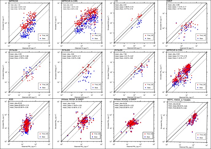
Scatterplots of observations versus simulation results from the averaged current time period Base_OAC and Final_OAC simulations for OC, TC, SOA, HOA, OOA, TOA, PM2.5, and PM10.
Figure 9.

A comparison of the monthly time series of OC and its components from selected sites in the IMPROVE and EMEP networks and monthly time series of TC and its components from the select sites in the CSN network from the Base_OAC, New_OAC, and Final_OAC simulations.
4.1.6. Multiple Parameter Sensitivity
OA_Final_Mix combines the configurations of the OA_LOW_Fragmentation, OA_LOW_WDEP, and OA_HVAP, because in general each configuration leads to the improvement of simulated OA against most evaluation metrics. POA levels are enhanced by 1.6 × 10⁻² µg m−3 on global average and by as much as 38.2 µg m−3 in the biomass burning regions of central Africa and South America (Figure 2.10). Unlike the majority of the sensitivity experiments, the changes in POA from OA_Final_Mix are statistically significant. The increases in POA lead to slight improvements in HOA performance, reducing the NMB from −36.4% in New_OA to −31.5%. OOA is enhanced by 0.17 µg m−3 on global average (Figure 3.10) with OA_Final_Mix. OOA is enhanced in the range of 0.2–1.0 µg m−3 across most continental areas. The enhancements are even larger (e.g., in the range of 1.0–12.4 µg m−3) over central Africa, central South America, Europe, East Asia, and eastern U.S. The increase in OOA leads to significantly improved OOA performance, reducing the NMB from −45.9% in New_OA to −27.0%. OA_Final_Mix provides a significant enhancement in the TOA level of 0.19 µg m−3 on global average, which is comparable to TOA increases from OA_NO_WDEP. This leads to increased model performance in most total OA metrics compared to New_OA. These include, a reduction in the underpredictions of European OC (its NMB changes from −52.4% to −29.2%), CONUS TC (its NMB changes from −37.4% to 12.3%), and NH TOA (its NMB changes from −51.5% to −38.6%) (Table 3). However, there is a degradation of CONUS OC performance from IMPROVE, with the NMB increasing from −0.3% to 45.7%. Nonetheless, the improvements across multiple OA metrics indicate that the configurations of OA_Final_Mix are an appropriate final configuration for the OA treatments. The remaining sensitivity simulations do not substantially impact the surface OA level but a detailed analysis of this sensitivity is presented in the supporting information.
Figure 10.

The relative contributions of HOA and OOA from selected sites in the Zhang et al. [2007] and Jimenez et al. [2009] data set and the relative contribution of the OA species from the CESM‐NCSU Base_OAC, New_OAC, and Final_OAC simulations.
4.2. Sensitivity of Aerosol/Climate Interactions
4.2.1. Impact of OOA Levels on Aerosol/Climate Interactions
The assumptions tested in OA_HVAP, OA_NO_WDEP, and OA_Final_Mix show a strong impact on cloud/radiative parameters. In order to examine this impact in greater detail, Figure 4 shows the zonally averaged vertical cross section of the absolute differences in OOA, CCN, CDNC, and particle number concentration between these simulations and New_OA. OOA increases by 0.05, 0.14, and 0.12 µg m−3 on vertical domain average in the OA_HVAP, OA_NO_WDEP, and OA_Final_Mix simulations, respectively. In OA_HVAP, the increases are the largest increases in the NH midlatitudes (e.g., 0.2–0.3 µg m−3 from the surface to roughly 750 mb). In the OA_NO_WDEP and OA_Final_Mix simulations OOA increases are largest from the surface to approximately 600 mb throughout most of the NH and tropics (15°S–60°N). Enhanced OOA increases CCN by 5.8, 17.8, and 13.1 cm−3 on vertical domain average in the OA_HVAP, OA_NO_WDEP, and OA_Final_Mix simulations, respectively.
Despite increasing CCN in all three simulations, there are different trends in the CDNC. In OA_NO_WDEP, the lack of SVOC wet deposition increases CDNC through increasing the size and hygroscopicity of preexisting aerosols and increases in the aerosol number (e.g., 2.9 × 102 cm−3 on vertical domain average) because of enhanced organic NPF from larger SVOC levels. The combination of these effects increases CDNC by 0.4 cm−3 on vertical domain average. OA_HVAP shows a very different impact on CDNC, with CDNC decreasing by 0.08 cm−3 on vertical domain average from a reduction of 1.6 × 102 cm−3 in particle number on vertical domain average. The particle number is reduced due to reductions in SVOCs from greater partitioning to the particulate phase, which decreases the rate of organic NPF. The overall impact on CDNC indicates that although the aerosols in OA_HVAP are likely larger in size and more hygroscopic, the reductions in particle number dominate the changes of CDNC. In OA_Final_Mix, the effect of the greater partitioning due to the use of E10 ΔHvap dominates, leading to a vertical domain average reduction of 1.5 × 102 cm−3 in particle number concentration. However, the greater increases in OOA in OA_Final_Mix compensate these reductions, leading to a complicated pattern in CDNC perturbations.
The combined impact of the CDNC, particle number concentration, and OOA enhancements in OA_NO_WDEP are global average increases in COT, SWCF, and AOD of 0.3, 1.4 W m−2, and 8.8 × 10⁻³, respectively, as shown in supporting information Figure S4. Compared to New_OA, these changes reduce underpredictions of AOD, COT, CCN, and LWP but increase overpredictions of CDNC and SWCF. In OA_HVAP, the increase in OOA increases AOD on global average by 3.7 × 10⁻³, however, decreases in CDNC decrease COT on global average. OA_Final_Mix also increases COT, SWCF, and AOD on global average by 0.19, 0.69 W m−2, and 7.7 × 10⁻³, respectively. Enhancements in cloud and radiative parameters in all three simulations indicate that both SVOC deposition and the choice of ΔHvap generate a strong climate signal by controlling both the direct and indirect OA effect.
4.2.2. Impact of OA κ Values on Aerosol/Climate Interactions
The OA_HI_κ and OA_LOW_κ simulations are performed to explore the impact of the OA hygroscopicity parameter κ on aerosol‐cloud interactions. The κ value changes the solubility of OA for the calculations of both aerosol activation and wet removal. Figure 5 shows the zonally averaged absolute differences in CCN, CDNC, and COT between OA_HI_κ or OA_LOW_κ and New_OA. The increased κ values in OA_HI_κ increase CCN on vertical domain average by 6.2 cm−3, while the reductions in κ values in OA_LOW_κ reduce CCN by 9.2 cm−3. Changes in CCN in both the OA_HI_κ and OA_LOW_κ simulations are the largest in the regions spanning the latitude range 15°S–60°N from the surface to 700 mb.
Changes in CDNC are more complex than changes in CCN; even though some of the patterns are discernible. In OA_HI_κ, the increased κ values increase CDNC by up to 3.9 cm−3 in clouds over the SH midlatitudes, largely from 40°S to 60°S, and the higher latitudes of the NH, from 60°N to 75°N. Increases in CCN in OA_HI_κ do not necessarily mean the CCN will activate to form cloud droplets. In OA_HI_κ, thermodynamic perturbations in the model result in decreased cloud fractions over much of the NH midlatitudes (figure not shown). This reduces the CDNC in this region even though CCN are increased. The reduced κ values for all of the OA species from OA_LOW_κ has a stronger impact on CDNC changes compared to OA_HI_κ, with reductions of 0.19 cm−3 on average and the largest reductions (1.5–5.8 cm−3) in clouds over the NH. The reductions in cloud fraction in OA_HI_κ dominate the changes in COT, leading to vertical domain average reductions. In OA_LOW_κ, COT is reduced by 9.1 × 10⁻³ on vertical domain average but up to 0.1–0.5 in midlatitude cloud of the NH and the lower latitudes of the SH. Although some patterns exist from changes in these vertical cross sections, the spatial distributions of the changes in COT, LWP, and SWCF shown in supporting information Figure S5 are highly complex and have a “noisy” appearance.
Interestingly the changes in CDNC, COT, LWP, and SWCF between both the OA_HI_κ and OA_LOW_κ simulations are very similar despite applying different forcing to the CCN concentration. This could potentially indicate that the original κ values for OA in CESM‐NCSU are the most optimum for aerosol activation and thus any change to the κ value will lead to similar results. CDNC is a function of many factors including updraft velocity, temperature, and aerosol properties. Therefore, even with different forcing applied to the κ value, similar changes could occur in thermodynamic and dynamic variables impacting simulated clouds. A more detailed study of the individual microphysical processed impacting CDNC would be needed to elucidate the reason for the similarity of the results in both simulations, which is an area of potential future work.
4.2.3. Impact of Organic NPF on Aerosol/Climate Interactions
The zonal‐averaged vertical cross section of the absolute difference in particle number, CCN, and CDNC between New_OA and OA_NO_ONPF or OA_SOA_ONPF is plotted in Figure 6 to illustrate the impact of the organic NPF treatment. The annual average nucleation rate (J) from the New_OA, OA_NO_ONPF, and OA_SOA_ONPF simulations with overlaid observations compiled in He and Zhang [2014] is shown in supporting information Figure S6. The overlay plots show that the organic NPF increases J over the continents bringing it closer toward the observations, however, caution must be executed in this comparison. The observed J values represent limited time periods on the order of days and thus are not representative of the annual average J which may vary substantially.
Figure 6.

The zonally averaged cross‐sectional differences in particle number concentrations, CCN at a supersaturation of 0.5%, and cloud droplet number concentrations between new OA simulation and (left) the OA_NO_ONPF simulation and (right) the OA_SOA_ONPF simulation.
In Figure 6, the sensitivity experiments are subtracted from the New_OA base simulation, unlike the other figures where the New_OA simulation is subtracted from the sensitivity experiment. The NPF treatment increases the number concentration by 5.6 × 102 cm−3 on vertical domain average with the greatest increases in lower latitudes and the NH midlatitudes of 1.0 × 10³ to 2.5 × 103 cm−3 from the surface to 500 mb. The impact of the SVOCs from oxidation of POA and IVOCs (POA‐based S‐IVOCs) is a much smaller vertical domain mean increase of 9.7 × 101 cm−3. The full organic NPF treatment increases CCN by 4.3 cm−3 on vertical domain average (Figure 6), while the OA_SOA_ONPF configuration decreases CCN by 0.8 cm−3 despite the strong enhancements (12–29.6 cm−3) in the lower and middle latitudes of the NH. The increased CCN from the full organic NPF treatment increases the CDNC level by 0.6 cm−3 on vertical domain average, with POA‐based S‐IVOCs alone resulting in an increase of 0.3 cm−3. Generally, the organic NPF treatment increases CCN by 3.0–66.3 cm−3 throughout the boundary layer (surface to 800 mb) of the lower and middle latitudes. The inclusion of the organic NPF treatment enhances COT, LWP, and SWCF on global average by 0.5, 1.7 g m−2, and 0.1 W m−2, respectively (supporting information Figure S7). While the spatial changes in these parameters are also “noisy,” as shown in supporting information Figure S7, there is a consistent impact with the greatest enhancements occurring in regions with high biogenic SVOCs. The impact from including POA‐based SVOCs for organic NPF is weaker. POA‐based SVOCs were not included in the original Fan et al. [2006] organic NPF treatment. Based on the above sensitivity analysis, anthropogenic and biogenic SVOCs still play a dominant role in the NPF treatment. Although these simulations demonstrate that organic NPF has an impact on aerosol indirect effects, one caveat is the simplistic and empirical nature of the organic NPF parameterization used in this work. Additionally, this NPF does not take into account extremely low‐volatility volatile organic compounds (ELVOCs). Recent research has shown that ELVOCs contribute to new particle formation in forested regions [Ehn et al., 2014]. More complex and physically based parameterizations should be considered in future work once they become available for 3‐D model implementation.
5. Impacts of New OA Treatments and Current Period Evaluation
5.1. Evaluation and Comparison of OC, TC, and TOA
Figure 7 shows the absolute difference plots of POA, SOA, OOA, TOA, PM2.5, AOD, Column Number Concentration (NUM), CCN, CDNC, COT, SWCF, and FSDS between the Base_OAC and Final_OAC simulations. Supporting information Table S7 shows the p‐values from a Student's t test analysis on the differences between Base_OAC and New_OAC or Final_OAC for variables shown in Figure 7. The t test analysis indicates that the difference in OA and cloud/radiation parameters is statistically significant at the 95% confidence level for all parameters. Globally the final configuration of the OA updates reduces POA by 0.22 μg m−3 on global average due to the POA volatility considered in the new treatments. SOA increases on global average (e.g., 0.21 μg m−3) as a result of the increased SOA partitioning from the photochemical aging process, increased mass from functionalization in the VBS treatment, a slight increase in the number of anthropogenic VOC precursors, and the addition of glyoxal SOA. In the SH, SOA is reduced by 0.3–2.2 μg m−3 primarily in the Amazon and Congo rainforests and Indonesia. This decrease could partially be the result of the SOA forming potential of ISOP being reduced in the New_OA treatment or inaccuracies in wet deposition. Further details on these potential impacts can be found in the supporting information. The total OOA (SOA + SVOA from oxidized POA and IVOCs) increases on global average by approximately 0.33 μg m−3 with the strongest impact in regions with high POA emissions. In the SH, the formation of SVOA somewhat compensates SOA reductions in biomass burning regions, leading to a smaller reduction or even a net increase in OOA. The impact of the final configuration of the new OA treatments on TOA is a global average increase of 0.11 μg m−3, with the increase in OOA dominating in the NHIR. Decreases occur in the SH and South Asia due to weaker increases in OOA, stronger decreases in POA, and loss of SOA in the Amazon.
Table 4 summarizes performance statistics for Base_OAC, New_OAC, and Final_OAC for all variables mentioned in section 3 in this work. Tables 5, 6, 7 compare performance statistics of OA, OC, HOA, OOA, and TOA from this work to those using various VBS treatments summarized in Table 1. Figure 8 shows scatterplots corresponding to OC, TC, SOA, HOA, OOA, TOA, PM2.5, and PM10 statistics between Base_OAC and Final_OAC. VOC precursors ISOP, TOL, and XYL are simulated rather poorly with moderate‐to‐large underpredictions ranging from −32.0 to −53.0%. One exception is European TOL, which has NMBs of 0.6–5.8%. In addition to the fairly large bias, the NMEs for the VOCs in all simulations are greater than 60% and all the R values are near zero, with the exception of CONUS ISOP which has an R value of ∼0.7 in all simulations. The poor VOC performance is likely the result of inaccuracies in the global VOC emissions inventory, BVOC emissions module [Holm et al., 2014], the VOC measurements [Blanchard and Hafner, 2004], the mapping of the VOCs to the different chemical species in CB05_GE, or the oxidant levels (e.g., O3) simulated by CESM‐NCSU [He et al., 2015]. CESM‐NCSU overpredicts O3 by roughly 16.2% over CONUS and 47.8% in Europe [He et al., 2015], indicating that there is an overabundance of oxidants that could be responsible for the underpredictions in VOC precursors. This overprediction has been attributed to both underpredictions of O3 titration by NOx and underpredictions of O3 deposition [He et al., 2015].
Table 4.
Statistical Performance Comparison of Base_OAC (Base), New OAC (New), and Final_OAC (Final) Simulations
| Variables | Region | Obs | Sim | MBa | NMBb | NMEc | Rd | ||||||||||
|---|---|---|---|---|---|---|---|---|---|---|---|---|---|---|---|---|---|
| Base | New | Final | Base | New | Final | Base | New | Final | Base | New | Final | Base | New | Final | |||
| OC (µg m−3) | CONUSe | 1.0 | 0.6 | 0.8 | 1.3 | −0.4 | −0.3 | 0.3 | −37.9 | −25.3 | 31.4 | 49.6 | 41.6 | 44.1 | 0.55 | 0.56 | 0.66 |
| Europef | 2.9 | 1.1 | 0.9 | 1.5 | −1.7 | −2.0 | −1.4 | −60.5 | −68.6 | −49.3 | 64.8 | 70.9 | 55.8 | 0.17 | 0.37 | 0.38 | |
| TC (µg m−3) | CONUSf | 2.5 | 1.3 | 1.5 | 2.5 | −1.1 | −1.0 | 0 | −46.0 | −38.7 | −0.7 | 51.1 | 46.7 | 37.5 | 0.53 | 0.57 | 0.59 |
| HOA (µg m−3) | NH | 2.1 | 2.2 | 0.8 | 0.8 | 0.1 | −1.3 | −1.2 | 5.7 | −62.1 | −59.2 | 41.8 | 67.2 | 66.0 | 0.94 | 0.78 | 0.91 |
| OOA (µg m−3) | NH | 4.8 | 0.5 | 2.3 | 3.5 | −4.4 | −2.6 | −1.3 | −90.0 | −52.8 | −27.3 | 90.0 | 53.2 | 33.6 | 0.48 | 0.92 | 0.89 |
| TOA (µg m−3) | NH | 7.9 | 2.5 | 3.0 | 4.3 | −5.4 | −4.9 | −3.6 | −68.3 | −61.9 | −45.5 | 69.2 | 62.5 | 50.8 | 0.87 | 0.89 | 0.82 |
| SOA (µg m−3) | CONUS | 2.9 | 1.0 | 2.1 | 4.5 | −1.9 | −0.8 | 1.6 | −66.0 | −26.3 | 53.2 | 66.0 | 46.3 | 53.2 | 0.72 | 0.12 | 0.72 |
| PM2.5 (µg m−3) | CONUS | 8.3 | 10.2 | 9.4 | 11.4 | 1.8 | 1.1 | 3.1 | 22.2 | 13.3 | 37.4 | 40.6 | 33.8 | 48.7 | 0.78 | 0.73 | 0.77 |
| Europe | 14.1 | 11.1 | 9.9 | 10.5 | −3.0 | −4.2 | −3.6 | −21.4 | −30.0 | −25.6 | 35.5 | 37.2 | 38.9 | 0.20 | 0.28 | 0.13 | |
| PM10 (µg m−3) | CONUS | 22.2 | 20.7 | 17.9 | 20.6 | −1.6 | −4.3 | −1.6 | −7.0 | −19.3 | −7.3 | 49.7 | 44.0 | 43.5 | 0.19 | 0.27 | 0.26 |
| Europe | 24.4 | 23.0 | 21.6 | 23.6 | −1.4 | −2.8 | −0.8 | −5.6 | −11.6 | −3.3 | 34.7 | 36.0 | 36.6 | 0.22 | 0.17 | 0.21 | |
| East Asia | 94.6 | 58.0 | 69.8 | 69.5 | −36.6 | −24.7 | −25.0 | −38.6 | −26.2 | −26.5 | 40.6 | 34.6 | 33.4 | 0.65 | 0.62 | 0.63 | |
| ISOP (ppt) | CONUS | 322.6 | 198.2 | 212.6 | 197.8 | −124.4 | −110.0 | −124.8 | −38.6 | −34.1 | −38.7 | 66.2 | 67.0 | 64.8 | 0.69 | 0.67 | 0.70 |
| Europe | 162.1 | 109.4 | 98.2 | 97.8 | −52.8 | −64.0 | −64.5 | −32.6 | −39.4 | −39.8 | 78.8 | 73.6 | 76.1 | −0.03 | 0.0 | −0.06 | |
| TOL (ppt) | CONUS | 734.2 | 355.1 | 342.2 | 349.3 | −379.0 | −392.0 | −384.9 | −51.6 | −53.4 | −52.4 | 69.2 | 69.7 | 69.3 | −0.16 | −0.15 | −0.15 |
| Europe | 250.5 | 265.2 | 252.0 | 259.8 | 14.7 | 1.5 | 9.2 | 5.8 | 0.6 | 3.7 | 63.4 | 59.3 | 62.1 | −0.08 | −0.06 | −0.10 | |
| XYL (ppt) | CONUS | 419.9 | 202.7 | 208.2 | 212.5 | −217.2 | −211.7 | −207.4 | −51.7 | −50.4 | −49.4 | 89.2 | 89.5 | 89.2 | −0.13 | −0.14 | −0.13 |
| AOD | Global | 0.16 | 0.18 | 0.11 | 0.12 | 0.02 | −0.05 | −0.03 | 15.8 | −31.7 | −19.9 | 35.4 | 46.0 | 41.4 | 0.60 | 0.58 | 0.62 |
| COT | Global | 17.0 | 9.6 | 9.9 | 10.3 | −7.4 | −7.1 | −6.7 | −43.4 | −41.5 | −39.2 | 57.9 | 57.0 | 56.2 | −0.11 | −0.09 | −0.10 |
| CCN (cm−2) | Ocean | 6.4 × 10⁸ | 5.8 × 10⁷ | 5.4 × 10⁷ | 7.2 × 10⁷ | −1.8 × 10⁸ | −1.9 × 10⁸ | −1.7 × 10⁸ | −73.6 | −77.6 | −70.4 | 73.6 | 77.6 | 70.4 | 0.15 | 0.15 | 0.14 |
| CDNC (cm−3) | Global | 108.5 | 166.0 | 177.4 | 180.4 | 57.4 | 68.8 | 71.9 | 52.9 | 63.4 | 66.2 | 70.3 | 79.2 | 81.4 | 0.56 | 0.55 | 0.53 |
| LWP (g m−2) | Ocean | 85.7 | 53.5 | 54.4 | 56.9 | −32.2 | −31.3 | −28.8 | −37.5 | −36.5 | −33.6 | 40.6 | 40.3 | 39.0 | 0.45 | 0.44 | 0.46 |
| SWCF (W m−2) | Global | −40.7 | −39.4 | −40.9 | −42.4 | −1.3 | 0.2 | 1.6 | −3.3 | 0.4 | 4.0 | 21.4 | 21.0 | 22.2 | 0.90 | 0.91 | 0.91 |
| FSDS (W m−2) | Global | 163.5 | 162.3 | 165.5 | 162.9 | −1.1 | 2.0 | −0.6 | −0.7 | 1.2 | −0.3 | 5.2 | 5.5 | 5.6 | 0.98 | 0.98 | 0.97 |
Mean bias (MB).
Normalized mean bias (NMB).
Normalized mean error (NME).
Correlation coefficient (R).
Assumes an OM:OC ratio of 1.8.
Assumes an OM:OC ratio of 1.4.
Table 5.
Comparison of Performance Statistics of OA Over CONUSa
| Obs. Network | Statistic | A12b | F10 | J11 | J13b | L08b | MP09b | S08b | S15 | W15c | This Workc |
|---|---|---|---|---|---|---|---|---|---|---|---|
| IMPROVE OC (CONUS) | MB (μg m−3) | −0.43 to 1.30 | −0.65 to −0.36 | −1.1 to 0.5 | N/A | 0.33–6.44 | 0.29 | −0.41 to 0.45 | −0.12 to 1.66h | N/A | −0.26 to 0.32 |
| MAE (µg m−3) | N/A | 0.92–0.95 | N/A | N/A | 1.11–6.45 | 0.72 | 0.79–1.00 | N/A | N/A | 0.42–0.45 | |
| FBd/NMBe | N/A | −0.41 to −0.26d | −0.98 to 0.03d | −30.0 to 2.0e | 0.21–1.06d | 0.17d | −0.02 to 0.27d | N/A | 60.5e | −0.38 to 0.19d/–25.3 to 31.5e | |
| FEf/NMEg | N/A | 0.49–0.55f | 0.52–1.04f | 41.0–47.0g | 0.45–1.06f | 0.39f | 0.38–0.44f | N/A | 83.0g | 0.33–0.50f/41.6–44.2g | |
| R | 0.55–0.65 | 0.66 | N/A | 0.46–0.50 | N/A | 0.62 | N/A | N/A | 0.57 | 0.56–0.65 | |
| CSN OCb/TCc (CONUS) | MB (µg m−3) | −1.77 to 0.57 | N/A | N/A | N/A | −1.23 to 3.60 | −0.88 | −2.24 to −0.95 | N/A | N/A | −0.96 to −0.02 |
| MAE (µg m−3) | N/A | N/A | N/A | N/A | 1.80–3.94 | 1.33 | 1.76–2.59 | N/A | N/A | 0.93–1.16 | |
| FBd/NMBe | N/A | N/A | N/A | N/A | −0.21 to 0.43d | −0.29d | −0.50 to −0.08d | N/A | 53.1e | −0.39 to 0.08d/–38.7 to −0.08e | |
| FEf/NMEg | N/A | N/A | N/A | N/A | 0.37–0.50f | 0.52f | 0.58–0.64f | N/A | 76.8g | 0.39–0.50f/37.5–46.7g | |
| R | 0.68–0.76 | N/A | N/A | N/A | N/A | 0.52 | N/A | N/A | 0.54 | 0.57–0.59 |
MB: mean bias, MAE: mean absolute error, FB: fractional bias, FE: fractional error, NMB: normalized mean bias, NME: normalized mean error, R: Pearson's correlation coefficient, A12: Ahmadov et al. [2012], F10: Farina et al. [2010], J11: Jathar et al. [2011], J13: Jo et al. [2013], L08: Lane et al. [2008], MP09: Murphy and Pandis [2009], S08: Shrivastava et al. [2008], S15: Shrivastava et al. [2015], and W15: Wang et al. [2015].
CSN statistics based on organic carbon.
CSN statistics based on total carbon.
FB.
NMB.
FE.
NME.
Statistics based on median bias rather than mean bias.
Table 6.
Comparison of Performance Statistics Against European EMEP OC Observationsa
Table 7.
Comparison of Performance Statistics Against Z07 and J09 Observationsa
| OA Type | Statistic | J13 | This Work |
|---|---|---|---|
| HOA | RMSE (µg m−3) | 3.11 | 2.54–2.60 |
| NMB | 85.0 | −59.2 to −62.1 | |
| NME | 107.0 | 66.0–67.2 | |
| R | 0.43 | 0.91 | |
| OOA | RMSE (µg m−3) | 3.47–3.92 | 2.27–3.30 |
| NMB | −71.0 to −43.0 | −52.0 to −27.3 | |
| NME | 61.0–76.0 | 33.6–53.2 | |
| R | 0.22–0.26 | 0.89–0.92 | |
| TOA | RMSE (µg m−3) | 4.26–4.44 | 4.01–7.11 |
| NMB | −8.0 to −29.0 | −61.9 to −45.5 | |
| NME | 58.0–62.0 | 50.8–62.5 | |
| R | 0.45–0.47 | 0.82–0.89 |
RMSE: root‐mean‐square error, NMB: normalized mean bias, NME: normalized mean error, R: Pearson's correlation coefficient, and J13: Jo et al. [2013].
OC statistics assuming OM:OC ratios of 1.8 are calculated for CONUS. The ratio of 1.4 is the typical assumption but 1.8 is a better assumption at the IMPROVE sites [Lane et al., 2008]. OC over CONUS in Base_OAC is moderately underpredicted by −37.9%. This underprediction is reduced in New_OAC and becomes a moderate overprediction of 31.4% in Final_OAC. The overprediction of CONUS OC is consistent with many regional VBS studies shown in Table 5. Simulation errors (i.e., NME) are reduced in New_OAC and Final_OAC. R in New_OAC is similar to Base_OAC, but R increases from 0.55 in Base_OAC to 0.66 in Final_OAC, indicating an improvement in spatial pattern. The performance of CONUS OC is comparable to that of other studies listed in Table 5 in terms of bias, errors, and R values. However, compared to the simulations from the other global modeling studies of Farina et al. [2010], Jathar et al. [2011], and Jo et al. [2013], New_OAC has smaller underprediction and Final_OAC has larger overprediction. The differences compared to the other global modeling studies are due to the inclusion of greater functionalization and aging of biogenic SVOCs in the CESM‐NCSU treatment. A more detailed discussion of VBS model performance from Table 5 can be found in the supporting information [Lane et al., 2008; Murphy and Pandis, 2009; Farina et al., 2010; Jathar et al., 2011; Ahmadov et al., 2012; Bergstrom et al., 2012; Jo et al., 2013; Shrivastava et al., 2013; 2015].
As shown in Table 4, there are improvements in simulated TC over CONUS with the new OA treatments. The magnitude of the NMB/NME is decreased from −46.0%/51.1% to −38.7%/47.6% in New_OAC, but the model improvement is even more significant in Final_OAC (with an NMB/NME of −0.7%/37.5%). There are only slight improvements in the R values from 0.53 in BASE_OAC to 0.57 and 0.59 in New_OAC and Final_OAC, respectively. This indicates that the new OA treatments improve TC more in terms of bias than spatial pattern. The scatterplots in Figure 8 show that CONUS OC and TC sites from Final_OAC are clustered much closer to the one‐to‐one line compared to those of Base_OAC, indicating an improvement in simulated OA over CONUS from the final configuration of the new OA treatments. The model performance in terms of bias and error for TC over CONUS is within the range of model performance of OC from CSN reported from previous studies in Table 5. However, there are some caveats to this comparison since TC over CONUS from CESM‐NCSU contains both the IMPROVE and CSN sites averaged together, due to the coarse resolution of CESM‐NCSU, instead of a pure CSN comparison reported in other studies.
In Europe, there is poor OC performance in all three simulations with NMBs of −60.5%, −68.6%, and −49.3% in Base_OAC, New_OAC, and Final_OAC, respectively, most likely because of errors in European emissions. This is evident in the smaller sensitivity of European OC performance compared to the other OA metrics evaluated and also by the poor R values from nearly all chemical species simulated over Europe from CESM‐NCSU [He et al., 2015]. Nonetheless, Final_OAC not only improves model performance in terms of bias but also improves the spatial evaluation of OC (e.g., increases in R from 0.17 to 0.38) (Table 4). The smaller R values and large underpredictions in European OC from CESM‐NCSU are consistent with most other VBS studies that evaluated against OC measurements from EMEP listed in Table 6. The only exception is Farina et al. [2010] which reports a large overprediction compared to EMEP measurements. This is likely because POA is treated as nonvolatile in Farina et al. [2010], allowing for greater levels of OC mass in the particulate phase.
Similarly, TOA is largely underpredicted in all simulations with NMBs of −68.3%, −61.9%, and −45.5% in BASE_OAC, New_OAC, and Final_OAC, respectively. Final_OAC also shows significant improvements in bias and NME (e.g., a decrease from 69.2% to 50.8%) (Table 4). The R values in all simulations are similar ranging from 0.82 to 0.89, with the new OA treatments reducing the R values slightly. Based on the scatterplot in Figure 8, a large number of the sites included in Z07 and J09 fall on or close to the one‐to‐one line in Final_OAC. Thus, the large NMB is the result of underpredicted OA at a few sites and a small overall sample size of 37. The underprediction of TOA is consistent with Jo et al. [2013] as shown in Table 7. However, the magnitude of the underprediction is larger in CESM‐NCSU since HOA in CESM‐NCSU is largely underpredicted.
Figure 9 compares observed and simulated monthly time series of TC and OC from Base_OAC, New_OAC, and Final_OAC at selected sites from CSN, IMPROVE, and EMEP. Overall, the Final_OAC configuration of the new OA treatments provides a much better representation of the magnitude and seasonal patterns of OA than Base_OAC of CESM‐NCSU. However, deviations from observations still exist. The most striking deviation is underpredicted OC and TC during the moths of January, February, and December, likely due to the underpredicted POA. TC at the PHO site indicates that regions dominated by BC and POA will not experience significant improvements in model performance from the new OA treatments. The time series analysis also reveals that the modifications to fragmentation, SVOC wet deposition, and ΔHvap values in Final_OAC do not improve model performance at all locations, as evidenced by the OC performance at GRSM. Deviations from observations such as those reported here have occurred in other VBS studies [Lane et al., 2008; Bergstrom et al., 2012], indicating that while the VBS framework for OA leads to improved performance compared to more traditional OA treatments, it may not be a “one size fits all” treatment and could benefit from the inclusion of other OA simulation techniques like those of the molecular approach. A more detailed analysis of Figure 9 can be found in the supporting information [Puxbaum et al., 2007; Yttri et al., 2007; Zhang et al., 2010].
5.2. Evaluation and Comparison of HOA, OOA, and SOA
OOA performance is significantly improved with the new OA treatments. OOA performance is extremely poor in Base_OAC, with an NMB of −90.0%, an NME of 90.0%, and an R value of 0.48. This performance is improved in both New_OAC and Final_OAC (i.e., NMBs of −52.8% and −27.3%, NMEs of 53.2% and 33.6%, and R values 0.92 and 0.89, respectively) (Table 4). The OOA performance of CESM‐NCSU is improved in terms of bias, error, and R values compared to Jo et al. [2013] as shown in Table 7. The improved performance of CESM‐NCSU is likely the result of the inclusion of the FT‐FG treatment and aging of biogenic SVOCs. HOA performance is degraded in terms of NMBs, changing from a slight 5.8% overprediction in Base_OAC to −62.1% and −59.2% underpredictions in New_OAC and Final_OAC, respectively. This indicates that POA in the VBS framework is too volatile. One potential reason for the underprediction of HOA is the rapid aging of POA from the primary carbon mode to the accumulation mode in MAM7. This aging has been indicated to lead to extremely efficient wet removal of POA [X. Liu et al., 2012]. In the VBS framework, the efficient wet removal of POA potentially leads to a feedback effect wherein the underpredicted particle‐phase POA level will reduce absorbing material and total POA mass biasing the POA to the gas‐phase. The HOA performance of CESM‐NCSU contrasts with the findings of Jo et al. [2013] shown in Table 7, which show a large overprediction compared to HOA measurements. This could be related to differences in emissions between both studies, and also due to the potential POA wet removal errors in CESM‐NCSU. Nonetheless, CESM‐NCSU has better performance in terms of errors and R values compared to the work of Jo et al. [2013].
Figure 10 compares the relative contributions of POA and OOA to TOA in Base_OAC, New_OAC, and Final_OAC against the relative contributions of HOA and OOA to TOA in the Z07 and J09 data set at selected sites. All three CESM‐NCSU simulations capture the decrease in relative contributions of POA from the urban to the rural sites. The OA treatments in Final_OAC significantly improve the simulation of POA/OOA speciation in CESM‐NCSU. Differences in the POA and OOA split between New_OAC and Final_OAC are not large. The configuration of Final_OAC increases the relative contributions of BSOA at the expense of POA and SVOA. The increased relative contribution of POA in New_OAC does not significantly impact model performance, as it improves model performance at some sites (e.g., Manchester) and degrades that at other sites (e.g., Duke Forest). More detailed discussion of the relative contributions of POA and OOA at each site can be found in the supporting information.
The impacts of the new OA treatments on SOA model performance are fairly complex. The NMB for SOA is reduced from a significant underprediction of −66.0% in Base_OAC to a more moderate underprediction of −26.3% in New_OAC. However, the NMB against the L13 SOA data becomes an overprediction of 53.2% in Final_OAC. It is important to note that caution must be used when interpreting these results, since simulated SOA and observed SOA are not diagnosed from the same VOC precursors. A more detailed description of this inconsistency can be found in the supplement. The increase in R values from 0.12 to 0.72 between New_OAC and Final_OAC illustrates the importance of reducing the SVOC wet deposition in Final_OAC and may also indicate that aqueous SOA formation processes neglected here play an important role in SOA formation. Because of the larger amount of anthropogenic precursors in the new OA treatments, CESM‐NCSU overpredicts SOA at the three California sites included in L13 (i.e., Pasadena, Bakersfield, and Riverside), where many ASOA precursors are available. In New_OAC, CESM‐NCSU underpredicts SOA at the sites from the Southeastern Aerosol Research and Characterization (SEARCH) network that are located in a largely BVOC dominated environment with high precipitation rates. This makes the R value small, since there is an overprediction in the region with low estimated SOA and a slight underprediction in the region with larger estimated SOA. In Final_OAC, SOA is still overpredicted at the California sites, but SOA at the SEARCH sites are also slightly overpredicted due to the reduction in SVOC wet deposition. This leads to a better R value between simulated and observed values.
Figure 11 compares the relative contributions of ASOA to BSOA at four sites in the L13 data set to those predicted by New_OAC and Final_OAC. A comparison was not possible from Base_OAC because all SOA are lumped into one species in the default OA treatments. The contributions of ASOA and BSOA at the RTP and Pensacola sites are similar between the L13 estimates and the CESM‐NCSU simulations. This is different from the Bakersfield and Detroit sites where estimated ASOA contributions are slightly greater than BSOA contributions, than those in the L13 data set. The values at all four sites are in relatively good agreement; however, it is difficult to attribute the differences at the low BVOC sites to errors in model performance. This is because the L13 data set uses only two anthropogenic SOA components to estimate ASOA, which creates biases in the L13 estimate toward BSOA even in urban areas that have high AVOCs. Detailed analysis of how the changes in OA impact PM2.5 and PM10 and a detailed speciation of OA in the various regions across the globe can be found in supporting information Text S12, Text S13, and Table S8 [Fuzzi et al., 2007; Fu et al., 2008; May et al., 2008; Stavrakou et al., 2009; X. Liu et al., 2012; Knote et al., 2014; He et al., 2015].
Figure 11.

The relative contributions of ASOA and BSOA from selected sites of the Lewandowski et al. [2013] data set and similar relative contributions at these sites from the CESM‐NCSU New_OAC and Final_OAC simulations.
5.3. Impacts and Evaluation of Aerosol/Climate Interactions
The addition of the organic NPF treatment increases the global NUM level by 3.0 × 1017 cm−2 on global average in Final_OAC. The impact is the strongest in the tropics and subtropics (30°S–30°N), where NUM increases by 8.0 × 10¹⁷ to 2.0 × 1018 cm−2 due to relatively high SVOC levels. The increase in NUM combined with the increase in OOA/TOA leads to a global average increase in CCN of 8.4 × 106 cm−2. The increases in CCN are the largest in eastern China, the southeastern U. S., central Africa, and South Asia (e.g., 4.0 × 10⁷ to 1.2 × 10⁸). These regions correspond to regions with the largest increases in OOA between Base_OAC and Final_OAC. The OOA impact on CCN is stronger than that of TOA for two primary reasons. The first is that POA is more hydrophobic than OOA in CESM‐NCSU, with a κ value of 0.1 compared to 0.14 for OOA species. Second, the POA in the primary carbon mode is both smaller and externally mixed from other aerosols, making them less likely to act as CCN. The increase in CCN, from either increased NUM or increases in OOA, increases global average CDNC by 10.2 cm−3. However, changes in CDNC are complex because increased CCN does not guarantee an increase in CDNC, as different feedbacks from chemistry into climate could impact cloud formation differently. In terms of model performance CCN is largely underpredicted in CESM‐NCSU with a −73.6% NMB in Base_OAC. This can be attributed to a lack of a marine organic aerosol treatment and errors in sea‐salt concentrations [He et al., 2015]. The NMB is improved slightly in Final_OAC to −70.4%. Model improvements in CCN are not dramatic, since the satellite estimate only exists in marine regions and the bulk of the CCN enhancements occur over continental environments. CDNC is largely overpredicted in BASE_OAC, with an NMB of 52.9%. This overprediction is enhanced in Final_OAC to an NMB of 66.2%. This overprediction could be attributed to either the aerosol activation updates in the work of Gantt et al. [2014] or due to a potential underestimate of CDNC by the Bennartz [2007] data set, from errors in the MODIS products used to derived these estimates [He et al., 2015].
AOD decreases nearly domain wide by 0.06 on global average in Final_OAC due to decreases in POA in the final configuration of the new OA treatments. The impact of reduced POA dominates because biomass burning emissions of POA are prescribed a vertical profile to mirror the injection of aerosol from fires at higher altitudes, resulting in a greater impact throughout the depth of the troposphere. The increase in CDNC from the new OA treatments increases the aerosol‐cloud lifetime effect, increasing LWP on global average by 2.8 g m−2 (figure not shown). This combined with increases in cloud albedo from increased CDNC result in an increase in COT of 0.7 on global average (Figure 7). AOD is overpredicted, with an NMB of 15.8% in Base_OAC, while AOD is underpredicted in Final_OAC with an NMB of −19.9%. This is a slight degradation in model performance that results from the POA being too volatile in the new OA treatments. LWP and COT are underpredicted in CESM‐NCSU, with NMBs of −37.5% and −43.2% in Base_OAC, respectively. This type of moderate underpredictions in cloud parameters is common in many global models [Lauer and Hamilton, 2013] and regional air quality models [Zhang et al., 2012a], indicating important limitations in simulating cloud properties that need to be addressed by the scientific community in order to better understand the indirect forcing of aerosols. The underpredictions in both LWP and COT are reduced in Final_OAC to −33.6% and −39.2%, respectively. These improvements in model performance are small but based on the Student's t test analysis they are statistically significant.
The enhancements in COT from the enhanced cloud albedo and cloud lifetime effects in Final_OAC lead to increases in SWCF of 2.9 W m−2 on global average. The increases are the largest in marine environments that have less CCN and greater LWP compared to continental clouds. These clouds are more sensitive to changes in aerosol levels than their continental counterparts. Thus, even though the new OA treatments have the strongest impact on continental aerosol levels, the strongest climate impact occurs in the marine environments. The increase in SWCF from increases OOA levels is compensated by the increase in FSDS from reductions in AOD. As a result, the global average change in FSDS is an increase of ∼0.6 W m−2 on global average. The absolute difference plot of FSDS between Base_OAC and Final_OAC shows that the AOD reduction dominates the changes in radiation over the continents, while the enhanced SWCF dominates the changes in FSDS in marine environments. SWCF is slightly underpredicted in Base_OAC with an MB of −1.3 W m−2 and slightly overpredicted with an MB of 1.6 W m−2 in Final_OAC. The magnitude of the bias is similar in both simulations, but slightly larger in Final_OAC. FSDS is also slightly underpredicted in Base_OAC by −1.1 W m−2, which is reduced slightly to an MB of −0.6 W m−2 in Final_OAC. These values are also very similar but with a slight improvement in Final_OAC due to the underprediction of AOD that compensates the overprediction in SWCF.
6. Conclusions
In this work, CESM‐NCSU, a modified version of CESM/CAM5.1, has been further improved in its capability in simulating organic aerosols. The new OA treatments implemented in CESM‐NCSU include a VBS approach for simulating OA from VOCs, POA, and SVOA formed from oxidized POA and emitted S‐IVOCs from combustion, a simplified treatment for SOA formation from glyoxal, and a treatment for the simulation of organic NPF with sulfuric acid. This work differs from many past VBS treatments in global models by accounting for both functionalization and fragmentation of SVOCs and by including the aging biogenic SVOCs. There are similarities between this work and the work of Shrivastava et al. [2015], but this work has a greater focus on the comprehensive evaluation of OA against surface observations and the impact of OA on cloud properties. The primary objective of both studies also differs, as the objective of this study is to develop a version of CESM to that can adequately represent OA and its climate interactions within the current atmosphere for use in future climate simulations, while the objective of Shrivastava et al. [2015] is to understand the implications of different OA formation processes on spatial distribution, loadings, and lifetime of OA.
Sensitivity analysis has been conducted on various parameters controlling the new OA treatment in CESM‐NCSU that affect both the prediction of OA and its impact on the climate system. The POA emission factors and conservative aging approaches used in previous studies have been shown to underpredict OA. The impact of wet deposition of SVOCs has the strongest impact on TOA compared to all other parameters examined, indicating that an accurate representation of this process is important for accurate simulation of OA and may also indicate cloud processing of OA is significant. The choice of ΔHvap values also shows a substantial impact on OA predictions, especially in the middle and higher latitudes of the NH where OA sources and the seasonality of temperatures are maximized. The amount of fragmentation considered in the VBS treatment also has a significant impact on TOA predictions similar to the findings of Shrivastava et al. [2015]. Ultimately, the sensitivity simulation that contains reduced SVOC wet deposition, reduced fragmentation, and the E10 ΔHvap values is chosen as the final configuration of the new OA updates. This adjustment is justified by improved model performance of most OA metrics and aerosol/cloud interaction variables. However, the choice of these parameters as the “best” modeling parameterizations is limited to the version of CESM‐NCSU used in this work and the horizontal grid spacing of the CESM‐NCSU simulations. For example, the need to reduce the wet deposition may not be necessary in future versions if the wet deposition scheme is updated and the responses of CESM aerosol‐cloud interactions may change with simulation resolution [Ma et al., 2015].
Assumptions regarding OA κ values are shown to impact the vertical domain averaged predictions of CCN by ±9.2 cm−3. However, the general impact on various cloud and radiation parameters from these changes is difficult to distinguish from other complex interactions. The organic NPF treatment shows an impact on simulated aerosol‐cloud interactions by enhancing mean levels of CCN, CDNC, COT, LWP, and SWCF. In addition to strong impacts on the surface OA predictions, the choices in enthalpies of vaporization and SVOC wet deposition affect the simulated OA and SVOC levels throughout the atmosphere, which in turn impact aerosol‐climate interactions. The relatively strong impacts of SVOC wet deposition and enthalpies of vaporization on the aerosol direct and indirect effects of OA indicate that constraining and providing the best representation of these parameters is critical in order to accurately simulate the impacts of OA on the climate system. The impact of OA on aerosol/cloud interactions would also be aided by the incorporation of a more detailed treatment for organic aerosol NPF.
A comparison of results from the final OA treatments in CESM‐NCSU with the unmodified model reveals that these final OA treatments increase OOA levels globally by 0.33 μg m−3 mainly in the NHIR due to the additional precursors and pathways for OOA formation, but decrease POA levels by 0.22 μg m−3 on global average from treating POA volatility. The simulation with the final OA treatments shows significantly improved model performance against European OC, CONUS TC, NH TOA, and NH OOA. There is only slight improvement in model performance for CONUS OC and SOA. There is a degradation in the OA performance of simulated POA against NH HOA measurements, due to treating POA volatility in the final OA treatments. This degradation may be worse than discussed in this work since biomass burning observations are not considered when evaluating POA. Overall, CESM‐NCSU with the final OA treatments provides a very good bulk representation of OA globally during the current climate period, but there are deviations from observations at specific locations and during certain seasons. The reduced POA level from POA volatility reduces the OA direct effect. However, the increase in OOA increases the OA indirect effect by increasing SWCF. The net impact of the new treatments is an increase in FSDS of 0.6 W m−2, indicating that the reduced OA direct effect dominates over the enhanced OA indirect effect.
In addition to limitations of the OA treatments and CESM‐NCSU mentioned above, the VBS treatments included in CESM‐NCSU have some general limitations. These include missing pathways for OA formation, such as SOA formation from aqueous processes and detailed treatments for oligomerization and acid‐catalyzed chemistry of glyoxal or other carbonyl species. This could be addressed in future work by attempting to hybrid the VBS approach with the molecular approach similar to the hydrophilic/hydrophobic organic aerosol model [Couvidat et al., 2012]. The VBS treatments shown here may also be limited by using a modified 1‐D basis set as the two‐dimensional basis set that simulates O:C ratio may be better suited to accurately represent OA hygroscopicity [Jimenez et al., 2009]. Another key limitation is that the VBS treatments generally assume that OA forms pseudo ideal solutions and behaves in much the same manner as a liquid. This has been shown to not be the case in certain situations such as when OA is coated by very hydrophobic organic substances [Vaden et al., 2011] or when certain types of OA behave like viscous semisolids [Virtanen et al., 2010]. Viscous semisolid OA has been shown to form under cooler and drier atmospheric conditions [Järvinen et al., 2016], and the global chemical transport study of Shrivastava et al. [2017] has shown the relevance of these OA components on long range transport of PAHs and cancer risks. The recent studies of Shrivastava et al. [2015, 2016, 2017] have overcome the above limitations of VBS by adding a parameterization of rapid oligomerization that converts SOA into an effectively nonvolatile semisolid particle after a short period of time. New science has also revealed greater removal of OA through photolysis and heterogeneous oxidation [Hodzic et al., 2016] and the ELVOCs from the oxidation of BVOCs [Ehn et al., 2014; Jokinen et al., 2015]. The inclusion of ELVOC products that irreversibly generate OA play a crucial role in atmospheric CCN production [Jokinen et al., 2015] and also may contribute to NPF in forested regions [Ehn et al., 2014]. Lastly, both the glyoxal, SVOC dry deposition, and organic NPF treatments used in this work are highly simplified with large uncertainties. These uncertainties likely make the glyoxal and NPF treatments upper limit estimations of the impacts from the processes they represent. In general, this work serves as the first stage to including these OA processes in CESM for climate scale simulations and these treatments will undoubtedly need future refinement to improve their accuracy and reduce the associated uncertainty. There are also some general uncertainties in the primary SVOC/IVOC emissions, the volatility distribution of these emissions, representing the anthropogenic POA emissions with gasoline‐based emissions fractions, and uncertainties in the emissions of anthropogenic, biomass burning, and biogenic aerosols and VOCs. Overall, despite these limitations, CESM‐NCSU with the finalized OA treatments can reasonably reproduce OA levels and aerosol/cloud interactions in the current atmosphere and has some relative improvements in these variables compared to the original OA treatment in CESM. Thus, CESM‐NCSU with updated OA treatments is as suitable for climate scale simulations as the original CESM. It is imperative that such OA treatment be included in global climate models such as CESM1.0.5/CAM5.1 since OA will likely become the most dominant aerosol species over time. This is due to enhanced biogenic VOC emissions and oxidation predicted under future climate and projected more rapid decrease in emissions of other aerosol precursors such as SO2 than POA and anthropogenic VOCs by the year 2100 [Heald et al., 2008]. A preliminary version of this treatment was used for such climate scale simulations and the results of that study can be found in Glotfelty et al. [2017] and Glotfelty and Zhang [2017].
7. Erratum
In the originally published version of this article, the acknowledgement was published incorrectly. The correct text is below. All errors have since been corrected, and this version may be considered the authoritative version of record.This work is supported in part by the National Sciences Foundation (NSF) Earth System Modeling Program grant AGS‐1049200 at NCSU and in part under Assistance Agreement no. RD835871 awarded by the US Environmental Protection Agency to Yale University. It has not been formally reviewed by EPA. The views expressed in this document are solely those of the SEARCH Center and do not necessarily reflect those of the Agency. EPA does not endorse any products or commercial services mentioned in this publication.
Supporting information
Supporting Information S1
Acknowledgments
This work is supported in part by the National Sciences Foundation (NSF) Earth System Modeling Program grant AGS‐1049200 at NCSU and in part under Assistance Agreement no. RD835871 awarded by the US Environmental Protection Agency to Yale University. It has not been formally reviewed by EPA. The views expressed in this document are solely those of the SEARCH Center and do not necessarily reflect those of the Agency. EPA does not endorse any products or commercial services mentioned in this publication. We acknowledge high‐performance computing support from Yellowstone (ark:/85065/d7wd3xhc) provided by NCAR's Computational and Information Systems Laboratory, sponsored by the National Science Foundation. MODIS data and CERES data were provided by NASA via http://ladsweb.nasa.gov/data/search.html and http://ceres.larc.nasa.gov/order_data.php, respectively. Other surface network data were downloaded from their respective web sites. AQMEII emissions for CONUS were prepared by U.S. EPA, Environment Canada, Mexican Secretariat of the Environment and Natural Resources, and National Institute of Ecology. AQMEII emissions for Europe are provided by Alessandra Balzarini, Research on Energy System (RES), Italy. MEIC emissions for China were provided by Qiang Zhang and Kebin He, Tsinghua University, China. For simulation results presented in this paper, please contact the corresponding author, Yang Zhang, at yzhang9@ncsu.edu.
Glotfelty, T. , He J., and Zhang Y. (2017), Improving organic aerosol treatments in CESM/CAM5: Development, application, and evaluation, J. Adv. Model. Earth Syst., 9, 1506–1539, doi:10.1002/2016MS000874.
This article was corrected on 20 JUL 2017. See the end of the full text for details.
References
- Adams, P. J. , Seinfeld J. H., and Koch D. M. (1999), Global concentrations of tropospheric sulfate, nitrate, and ammonium aerosol simulated in a general circulation model, J. Geophys. Res., 104(D11), 13,791–13,823, doi:10.1029/1999JD900083. [Google Scholar]
- Ahmadov, R. , et al. (2012), A volatility basis set model for summertime secondary organic aerosols over the eastern United States in 2006, J. Geophys. Res., 117, D06301, doi:10.1029/2011JD016831. [Google Scholar]
- Aiken, A. C. , et al., (2008), O/C and OM/OC ratios of primary, secondary, and ambient organic aerosols with high‐resolution time‐of‐flight aerosol mass spectrometry, Environ. Sci. Technol., 42, 4478–4485, doi:10.1021/es703009q. [DOI] [PubMed] [Google Scholar]
- Barahona, D. , West R. E. I., Steir P., Romakkaniemi S., Kokkola H., and Nenes A. (2010), Comprehensively accounting for the effect of giant CCN in cloud activation parameterizations, Atmos. Chem. Phys., 10, 2467–2473, doi:10.1029/2006JD007547. [Google Scholar]
- Barth, M. C. , Rasch P. J., Kiehl J. T., Benkovitz C. M., and Schwartz S. E. (2000), Sulfur chemistry in the National Center for Atmospheric Research Community Climate Model: Description, evaluation, features and sensitivity to aqueous chemistry, J. Geophys. Res., 105(D1), 1387–1415, doi:10.1029/1999JD900773. [Google Scholar]
- Bennartz, R. (2007), Global assessment of marine boundary layer cloud droplet number concentration from satellite, J. Geophys. Res., 112, D02201, doi:10.1029/2006JD007547. [Google Scholar]
- Bergstrom, R. , Denier van der Gon H. A. C., Prevor A. S. H., Yttri K. E., and Simpson D. (2012), Modelling of organic aerosols over Europe (2002–2007) using a volatility basis set (VBS) framework: Supplication of different assumptions regarding the formation of secondary organic aerosols, Atmos. Chem. Phys., 12, 8499–8527, doi:10.5194/acp-12-8499-2012. [Google Scholar]
- Bessagnet, B. , Seigneur C., and Menut L. (2010), Impact of dry deposition of semi‐volatile organic compounds on secondary organic aerosol, Atmos. Environ., 44, 1781–1787, doi:10.1016/j.atmosenv.2010.01.027. [Google Scholar]
- Blanchard, C. L. , and Hafner H. R. (2004), SCAQMD PAMS assessment review task 1: Literature review, Rep. STI‐904042–2569‐TM, Sonoma Technol. Inc., Petaluma, Calif.
- Bretherton, C. S. and Park S. (2009), A new moist turbulence parameterization in the community atmosphere model, J. Clim., 22, 3422–3448, doi:10.1175/2008JCLI2556.1. [Google Scholar]
- Chan, A. W. H. , Kautzman K. E., Chhabra P. S., Surratt J. D., Chan M. N., Crounse J. D., Kurten A., Wennberg P. O., Flagan R. C., and Seinfeld J. H. (2009), Secondary organic aerosol formation from photooxidation of naphthalene and alkylnaphthalenes: Implications for oxidation of intermediate volatility organic compounds (IVOCs), Atmos. Chem. Phys., 9, 3049–3060, doi:10.5194/acp-9-3049-2009. [Google Scholar]
- Chung, S. H. , and Seinfeld J. H. (2002), Global distribution and climate forcing of carbonaceous aerosols, J. Geophys. Res., 107(D19), 4407, doi:10.1029/2001JD001397. [Google Scholar]
- Couvidat, F. , and Sartelet K. (2014), The Secondary Organic Aerosol Processor (SOAP v1.0) model: A unified model with different ranges of complexity based on the molecular surrogate approach, Geosci. Model Dev. Discuss., 7, 379–429, doi:10.5194/gmdd-7-379-2014. [Google Scholar]
- Couvidat, F. , Debry É., Sartelet K., and Seigneur C. (2012), A hydrophilic/hydrophobic organic (H2O) aerosol model: Development, evaluation and sensitivity analysis, J. Geophys. Res., 117, D10304, doi:10.1029/2011JD017214. [Google Scholar]
- Donahue, N. M. , Robinson A. L., Stanier C. O., and Pandis S. N. (2006), Coupled partitioning, dilution, and chemical aging of semivolatile organics, Environ. Sci. Technol., 40, 2635–2643, doi:10.1021/es052297c. [DOI] [PubMed] [Google Scholar]
- Donahue, N. M. , Robinson A. L., and Pandis S. (2009), Atmospheric organic particulate matter: From smoke to secondary organic aerosol, Atmos. Environ., 43, 94–106, doi:10.1016/j.atmosenv.2008.09.055. [Google Scholar]
- Donahue, N. M. , Epstein S. A., Pandis S. N., and Robinson A. I. (2011), A two‐dimensional volatility basis set: Organic‐aerosol mixing thermodynamics, Atmos. Chem. Phys., 11, 3303–3318, doi:10.5194/acp-11-3303-2011. [Google Scholar]
- Ehn, M. , et al. (2014), A large source of low‐volatility secondary organic aerosol, Nature, 506, 476–479, doi:10.1038/nature13032. [DOI] [PubMed] [Google Scholar]
- Emmons, L. K. , et al. (2010), Description and evaluation of the Modal for Ozone and Related Chemical Tracers, version 4 (MOZART‐4), Geosci. Model Dev., 3, 43–67, doi:10.5194/gmd-3-43-2010. [Google Scholar]
- Epstein, S. A. , Riipinen I., and Donahue N. M. (2010), A semiempirical correlation between enthalpy of vaporization and saturation concentration for organic aerosol, Environ. Sci. Technol., 44, 743–748, doi:10.1021/es902497z. [DOI] [PubMed] [Google Scholar]
- Ervens, B. , and Volkamer R. (2010), Glyoxal processing by aerosol multiphase chemistry: Towards a kinetic modeling framework of secondary organic aerosol formation in aqueous particles, Atmos. Chem. Phys., 10, 8219–8244, doi:10.5194/acp-10-8219-2010. [Google Scholar]
- Ervens, B. , Carlton A. G., Turpin B. J., Altieri K. E., Kreidenweis S. M., and Feingold G. (2008), Secondary organic aerosol yields from cloud‐processing of isoprene oxidation products, Geophys. Res. Lett., 35, L02816, doi:10.1029/2007GL031828. [Google Scholar]
- Fan, J. , Zhang R., Collins D., and Li G. (2006), Contribution of secondary condensable organics to new particle formation: A case study in Houston, Texas, Geophys. Res. Lett., 33, L15802, doi:10.1029/2006GL026295. [Google Scholar]
- Farina, S. C. , Adams P. J., and Pandis S. N. (2010), Modeling global secondary organic aerosol formation and processing with the volatility basis set: Implications for anthropogenic secondary organic aerosol, J. Geophys. Res., 115, D09202, doi:10.1029/2009JD013046. [Google Scholar]
- Fountoukis, C. , and Nenes A. (2005), Continued development of a cloud droplet formation parameterization for global climate models, J. Geophys. Res., 110, D11212, doi:10.1029/2004JD005591. [Google Scholar]
- Fountoukis, C. , and Nenes A. (2007), ISORROPIA II: A computationally efficient thermodynamic equilibrium model for K+‐Ca2+‐Mg2+‐ ‐Na+‐ ‐ ‐Cl–‐H2O aerosols, Atmos. Chem. Phys., 7, 4639–4659, doi:10.5194/acp-7-4639-2007. [Google Scholar]
- Fu, T.‐M. , Jacob D. J., Wittrock F., Burrows J. P., Vrekoussis M., and Henze D. K. (2008), Global budgets of atmospheric glyoxal and methylglyoxal, and implications for formation of secondary organic aerosols, J. Geophys. Res., 113, D15303, doi:10.1029/2007JD009505. [Google Scholar]
- Fuzzi, S. , et al. (2007), Overview of the inorganic and organic composition of size‐segregated aerosol in Rondônia, Brazil, from the biomass‐burning period to the onset of the wet season, J. Geophys. Res., 112, D01201, doi:10.1029/2005JD006741. [Google Scholar]
- Gantt, B. , He J., Zhang X., Zhang Y., and Nenes A. (2014), Incorporation of advanced aerosol activation treatments into CESM/CAM5: Model evaluation and impact on aerosol indirect effects, Atmos. Chem. Phys., 14, 7485–7497, doi:10.5194/acp-14-7485-2014. [Google Scholar]
- Gaydos, T. M. , Pinder R. W., Koo B., Fahey K. M., and Pandis S. N. (2007), Development and application of a three‐dimensional aerosol chemical transport model, PMCAMx, Atmos. Environ., 41, 2594–2611, doi:10.1016/j.atmosenv.2006.11.034. [Google Scholar]
- Glotfelty, T. , and Zhang Y. (2017), The impact of future climate policy scenarios on air quality and aerosol/cloud interactions using an advanced version of CESM/CAM5: Part II. Future trend analysis and impacts of projected anthropogenic emissions, Atmos. Environ., 152, 531–552, doi:10.1016/j.atmosenv.2016.12.034. [Google Scholar]
- Glotfelty, T. , He J., and Zhang Y. (2017), The impact of future climate policy scenarios on air quality and aerosol/cloud interactions using an advanced version of CESM/CAM5: Part I. Model evaluation for the current decadal simulations, Atmos. Environ., 152, 222–239, doi:10.1016/j.atmosenv.2016.12.035. [Google Scholar]
- Granier, C. , et al. (2005), POET, a database of surface emissions of ozone precursors [Available at http://www.aero.jussieu.fr/project/ACCENT/POET.php.]
- Grell, G. A. , Peckham S. E., Schmitz R., McKeen S. A., Frost G., Skamarock W. C., and Eder B. (2005), Fully coupled “online” chemistry within the WRF model, Atmos. Environ., 39(37), 6957–6975, doi:10.1016/j.atmosenv.2005.04.027. [Google Scholar]
- Grieshop, A. P. , Logue J. M., Donahue N. M., and Robinson A. L. (2009), Laboratory investigation of photochemical oxidation of organic aerosol from wood fires 1: Measurements and simulation of organic aerosol evolution, Atmos. Chem. Phys., 9, 1283–1277, doi:10.5194/acp-9-1263-2009. [Google Scholar]
- Guenther, A. , Karl T., Harley P., Wiedinmyer C., Palmer P. I., and Geron C. (2006), Estimates of global terrestrial isoprene emissions using MEGAN (Model of emissions of gases and aerosols from nature), Atmos. Chem. Phys., 6, 3181–3210, doi: 10.5194/acp-6-3181-2006. [Google Scholar]
- He, J. , and Zhang Y. (2014), Improvement and further development in CESM/CAM5: Gas‐phase chemistry and inorganic aerosol treatments, Atmos. Chem. Phys., 14, 9171–9200, doi:10.5194/acp-14-9171-2014. [Google Scholar]
- He, J. , Zhang Y., Glotfelty T., He R., Bennartz R., Rausch J., and Sartelet K. (2015), Decadal simulation and comprehensive evaluation of CESM/CAM5.1 with advanced chemistry, aerosol microphysics, and aerosol‐cloud interactions, J. Adv. Model. Earth Syst., 7, 110–141, doi:10.1002/2014MS000360. [Google Scholar]
- Heald, C. L. , et al. (2008), Predicted change in global secondary organic aerosol concentrations in response to future climate, emissions, and land use change, J. Geophys. Res., 113, D05211, doi:10.1029/2007JD009092. [Google Scholar]
- Hennigan, C. J. , Bergin M. H., Dibb J. E., and Weber R. J. (2008), Enhanced secondary organic aerosol formation due to water uptake by fine particles, Geophys. Res. Lett., 35, L18801, doi:10.1029/2008GL035046. [Google Scholar]
- Hodzic, A. , Kasibhatla P. S., Jo D. S., Cappa C. D., J. L., Jimenez , Madronich S., and Park R. J. (2016), Rethinking the global secondary organic aerosol (SOA) budget: Stronger production, faster removal, shorter lifetime, Atmos. Chem. Phys., 16, 7917–7941, doi:10.5194/acp-16-7917-2016. [Google Scholar]
- Holm, J. A. , Jardine K., Guenther A. B., Chambers J. Q., and Tribuzy E. (2014), Evaluation of MEGAN‐CLM parameter sensitivity to predictions of isoprene emissions from an Amazonian rainforest, Atmos. Chem. Phys. Discuss., 14, 23,995–24,041, doi:10.5194/acpd-14-23995-2014. [Google Scholar]
- Horowitz, L. W. , et al. (2003), A global simulation of tropospheric ozone and related tracers: Description and evaluation of MOZART, version 2, J. Geophys. Res., 108(D24), 4784, doi:10.1029/2002JD002853. [Google Scholar]
- Iacono, M. J. , Delamere J. S., Mlawer E. J., and Clough S. A. (2003), Evaluation of upper tropospheric water vapor in the NCAR Community Climate Model (CCM3) using modeled and observed HIRS radiances, J. Geophys. Res., 108(D2), 4037, doi:10.1029/2002JD002539. [Google Scholar]
- Iacono, M. J. , Delamere J. S., Mlawer E. J., Shephard M. W., Clough S. A., and Collins W. D. (2008), Radiative forcing by long‐lived greenhouse gases: Calculations with the AER radiative transfer models, J. Geophys. Res., 113, D13103, doi:10.1029/2008JD009944. [Google Scholar]
- Järvinen, E. , et al. (2016), Observation of viscosity transition in α‐pinene secondary organic aerosol, Atmos. Chem. Phys., 16(7), 4423–4438, doi:10.5194/acp-16-4423-2016. [Google Scholar]
- Jathar, S. H. , Farina S. C., Robinson A. L., and Adams P. J. (2011), The influence of semi‐volatile and reactive primary emissions on the abundance and properties of global organic aerosol, Atmos. Chem. Phys., 11, 7727–7746, doi:10.5194/acp-11-7727-2011. [Google Scholar]
- Jimenez, J. L. , et al. (2009), Evolution of organic aerosols in the atmosphere, Science, 326, 1525–1529, doi:10.1126/science.1180353. [DOI] [PubMed] [Google Scholar]
- Jo, D. S. , Park R. J., Kim M. J., and Spracklen D. V. (2013), Effects of chemical aging on global secondary organic aerosol using the volatility basis set approach, Atmos. Environ., 81, 230–244, doi:10.1016/j.atmosenv.2013.08.055. [Google Scholar]
- Jokinen, T. , et al. (2015), Production of extremely low volatility organic compounds from biogenic emissions: Measured yields and atmospheric implications, Proc. Natl. Acad. Sci. U. S. A., 112(23), 7123–7128, doi:10.1073/pnas.1423977112. [DOI] [PMC free article] [PubMed] [Google Scholar]
- Karamchandani, P. , Zhang Y., Chen S. Y., and Balmori‐Bronson R. (2012), Development and testing of an extended chemical mechanism for global‐through‐urban applications, Atmos. Pollut. Res., 3(1), 1–24, doi:10.5094/APR.2011.047. [Google Scholar]
- Knote, C. , et al. (2014), Simulation of semi‐explicit mechanisms of SOA formation from glyoxal in aerosol in a 3‐D model, Atmos. Chem. Phys., 14, 6213–6239, doi:10.5194/acp-14-6213-2014. [Google Scholar]
- Koo, B. , Knipping E., and Yarwood G. (2014), 1.5‐Dimensional volatility basis set approach for modeling organic aerosol in CAMx and CMAQ, Atmos. Environ., 95, 158–194, doi:10.1016/j.atmosenv.2014.06.031. [Google Scholar]
- Koo, B. Y. , Ansari A. S., and Pandis S. N. (2003), Integrated approaches to modeling the organic and inorganic atmospheric aerosol components, Atmos. Environ., 37, 4757–4768, doi:10.1016/j.atmosenv.2003.08.016. [Google Scholar]
- Kroll, J. H. , et al. (2011), Carbon oxidation state as a metric for describing the chemistry of atmospheric organic aerosol, Nat. Chem., 3, 133–139, doi:10.1038/nchem.948. [DOI] [PubMed] [Google Scholar]
- Kumar, P. , Sokolik I. N., and Nenes A. (2009), Parameterization of cloud droplet formation for global and regional models: Including adsorption activation from insoluble CCN, Atmos. Chem. Phys., 9, 2517–2532, doi:10.5194/acp-9-2517-2009. [Google Scholar]
- Lamarque, J.‐F. , et al. (2012), CAM‐Chem: Description and evaluation of interactive atmospheric chemistry in CESM, Geosci. Model Dev., 5, 369–411, doi:10.5194/gmd-5-369-2012. [Google Scholar]
- Lane, T. E. , Donahue N. M., and Pandis S. N. (2008), Simulating secondary organic aerosol formation using the volatility basis‐set approach in a chemical transport model, Atmos. Environ., 42(32), 7439–7451, doi:10.1016/j.atmosenv.2008.06.026. [Google Scholar]
- Lauer, A. , and Hamilton K. (2013), Simulating clouds with global climate models: A comparison of CMIP5 results with CMIP3 and satellite data, J. Clim., 26, 3833–3845, doi:10.1175/JCLI-D-12-00451.1. [Google Scholar]
- Lewandowski, M. , Piletic I. R., Kleindienst T. E., Offenberg J. H., Beaver M. R., Jaoui M., Docherty K. S., and Edney E. O. (2013), Secondary organic aerosol characterisation at field sites across the United States during the spring‐summer period, Int. J. Environ. Anal. Chem., 93, 1084–1103, doi:10.1080/03067319.2013.803545. [Google Scholar]
- Li, Y. J. , Lee B. T. L., Yu J. Z., Ng N. L., and Chang C. K. (2013), Evaluating the degree of oxygenation of organic aerosol during foggy and hazy days in Hong Kong using high‐resolution time‐of‐flight aerosol mass spectrometry (HR‐ToF‐AMS), Atmos. Chem. Phys., 13, 8739–8753, doi:10.5194/acp-13-8739-2013. [Google Scholar]
- Liao, H. , Adams P., Chung S., Seinfeld J., Mickley L., and Jacob D. (2003), Interactions between tropospheric chemistry and aerosols in a unified general circulation model, J. Geophys. Res., 108, D14001, doi:10.1029/2001JD001260. [Google Scholar]
- Liao, H. , Seinfeld J., Adams P., and Mickley L. (2004), Global radiative forcing of coupled tropospheric ozone and aerosols in a unified general circulation model, J. Geophys. Res., 109, D16207, doi:10.1029/2003JD004456. [Google Scholar]
- Lin, G. , Penner J. E., Flanner M. G., Sillman S., Xu L., and Zhou C. (2014), Radiative forcing of organic aerosol in the atmosphere and on snow: Effects of SOA and brown carbon, J. Geophys. Res. Atmos., 119, 7453–7476, doi:10.1002/2013JD021186. [Google Scholar]
- Liu, G. , Penner J. E., Sillman S., Taraborrelli D., and Lelieveld J. (2012), Global modeling of SOA formation from dicarbonyls, epoxides, organic nitrates, and peroxides, Atmos. Chem. Phys., 12, 4743–4774, doi:10.5194/acp-12-4743-2012. [Google Scholar]
- Liu, X. , and Penner J. E. (2005), Ice nucleation parameterization for global models, Meteorol. Z., 14, 499–514, doi:10.1127/0941-2948/2005/0059. [Google Scholar]
- Liu, X. , and Wang J. (2010), How important is aerosol hygroscopicity to aerosol indirect forcing?, Environ. Res. Lett., 5, 044010, doi:10.1088/1748-9326/5/4/044010. [Google Scholar]
- Liu, X. , et al. (2012), Toward a minimal representation of aerosols in climate models: Description and evaluation in the Community Atmosphere Model CAM5, Geosci. Model Dev., 5, 709–739, doi:10.5194/gmd-5-709-2012. [Google Scholar]
- Liu, Y. , Siekmann F., Renard P., El Zein A., Salque G., El Haddad I., Temime‐Roussel B., Voisin D., Thissen R., and Monod A. (2012), Oligomer and SOA formation through aqueous phase photooxidation of methacrolein and methyl vinyl ketone, Atmos. Environ., 49, 123–129, doi:10.1016/j.atmosenv.2011.12.012. [Google Scholar]
- Ma, P.‐L. , Rasch P. J., Wang M., Wang H., Ghan S. J., Easter R. C., Gustafson W. I. Jr., Liu X., Zhang Y., and Ma H.‐Y. (2015), How does increasing horizontal resolution in a global climate model improve the simulation of aerosol‐cloud interactions?, Geophys. Res. Lett., 42, 5058–5065, doi:10.1002/2015GL064183. [Google Scholar]
- Martensson, E. M. , Nilsson E. D., deLeeuw G., Cohen L. H., and Hansson H. C. (2003), Laboratory simulations and parameterizations of the primary marine aerosol production, J. Geophys. Res., 108(D9), 4297, doi:10.1029/2002JD0022263. [Google Scholar]
- May, A. A. , Presto A. A., Hennigan C. J., Nguyen N. T., Gordon T. D., and Robinon A. L. (2013a), Gas‐particle partitioning of primary organic aerosol emissions: (1) Gasoline vehicle exhaust, Atmos. Environ., 77, 128–139, doi:10.1016/j.atmosenv.2013.04.060. [DOI] [PubMed] [Google Scholar]
- May, A. A. , Levin E. J. T., Hennigan C. J., Riipinen I., Lee T., Collett J. L. Jr., Jimenez J. L., Kreidenweis S. M., and Robinson A. L. (2013b), Gas‐particle partitioning of primary organic aerosol emissions: 3. Biomass burning, J. Geophys. Res. Atmos., 118, 11,327–11,338, doi:10.1002/jgrd.50828. [Google Scholar]
- May, B. , Wagenbach D., Hammer S., Steier P., Pauxbaum H., and Pio C. (2008), The anthropogenic influence on carbonaceous aerosol in the European background. Tellus Ser. B, 61, 464–472, doi:10.1111/j.1600-0889.2008.00379.x. [Google Scholar]
- Mickley, L. J. , Murti P. P., Jacob D. J., Logan J. A., Koch D. M., and Rind D. (1999), Radiative forcing from tropospheric ozone calculated with a unified chemistry‐climate model, J. Geophys. Res., 104(D23), 30,153–30,172, doi:10.1029/1999JD900439. [Google Scholar]
- Morrison, H. and Gettelman A. (2008), A new two‐moment bulk stratiform cloud microphysics scheme in the community atmosphere model, version 3 (CAM3). Part I: Description and numerical tests, J. Clim., 21, 3642–3659, doi:10.1175/2008JCLI2105.1. [Google Scholar]
- Murphy, B. N. , and Pandis S. N. (2009), Simulating the formation of semivolatile primary and secondary organic aerosol in a regional chemical transport model, Environ. Sci. Technol., 43(13), 4722–4728, doi:10.1021/es803168a. [DOI] [PubMed] [Google Scholar]
- Murphy, B. N. , Donahue N. M., Fountoukis C., and Pandis S. N. (2011), Simulating the oxygen content of ambient organic aerosol with the 2D volatility basis set, Atmos. Chem. Phys., 11, 7859–7873, doi:10.5194/acp-11-7859-2011. [Google Scholar]
- Neale, R. B. , Richter J. H. and Jochum M. (2008), The impact of convection on ENSO: From a delayed oscillator to a series of events, J. Clim., 21, 5904–5924, doi:10.1175/2008JCLI2244.1. [Google Scholar]
- Nenes, A. , Pandis S. N., and Pilinis C. (1999), Continued development and testing of a new thermodynamic aerosol module for urban and regional air quality models, Atmos. Environ., 33(10), 1553–1560, doi:10.1016/S1352-2310(98)00352-5. [Google Scholar]
- Neu, J. L. , and Prather M. J. (2012), Toward a more physical representation of precipitation scavenging in global chemistry models: Cloud overlap and ice physics and their impact on tropospheric ozone, Atmos. Chem. Phys., 12, 3289–3310, doi:10.5194/acp-12-3289-2012. [Google Scholar]
- O'Dell, C. W. , Wentz F. J., and Bennartz R. (2008), Cloud liquid water path from satellite‐based passive microwave observations: A new climatology over the global oceans, J. Clim., 21, 1721–1739, doi:10.1175/2007JCLI1958.1. [Google Scholar]
- Odum, J. R. , Hoffmann T., Bowman F., Collins D., Flagan R. C., and Seinfeld J. H. (1996) Gas/particle partitioning and secondary organic aerosol yields, Environ. Sci. Technol., 30, 2580–2585, doi:10.1021/es950943+. [Google Scholar]
- Park, S. and Bretherton C. S. (2009), The University of Washington shallow convection and moist turbulence schemes and their impact on climate simulations with the community atmosphere model, J. Clim., 22, 3449–3469, doi:10.1175/2008JCLI2557.1. [Google Scholar]
- Park, S. , Bretherton C. S., and Rasch P. J. (2014), Integrating cloud processes in the Community Atmosphere Model, Version 5, J. Clim., 27, 6821–6856, doi:10.1175/JCLI-D-14-00087.1. [Google Scholar]
- Puxbaum, H. , Caseiro A., Sanchex‐Ochoa A., Kasper‐Giebl A., Claeys M., Gelencser A., Legrand M., Preunkert S., and Pio C. (2007), Levoglucosan levels at background sites in Europe for assessing the impact of biomass combustion on the European aerosol background, J. Geophys. Res., 112, D23S05, doi:10.1029/2006JD008114. [Google Scholar]
- Pye, H. O. T. and Seinfeld J. H. (2010), A global perspective on aerosol from low‐volatility organic compounds, Atmos. Chem. Phys., 10, 4377–4401, doi:10.5194/acp-10-4377-2010. [Google Scholar]
- Robinson, A. L. , et al., (2007), Rethinking organic aerosols: Semivolatile emissions and photochemical aging, Science, 315, 1259–1262, doi:10.1126/science.1133061. [DOI] [PubMed] [Google Scholar]
- Schell, B. , Ackermann I. J., Hass H., Binkowski F. S., and Ebel A. (2001), Modeling the formation of secondary organic aerosol within a comprehensive air quality model system, J. Geophys. Res., 106(D22), 28,275–28,293, doi:10.1029/2001JD000384. [Google Scholar]
- Shrivastava, M. K. , Lane T. E., Donahue N. M., Pandis S. N., and Robinson A. L. (2008), Effects of gas particle partitioning and aging of primary emissions on urban and regional organic aerosol concentrations, J. Geophys. Res., 113, D18301, doi:10.1029/2007JD009735. [Google Scholar]
- Shrivastava, M. K. , Fast J., Easter R., Gustafson W. I. Jr., Zaveri R. A., Jimenez J. L., Saide P., and Hodzic A. (2011), Modeling organic aerosols in a megacity: Comparison of simple and complex representations of the volatility basis set approach, Atmos. Chem. Phys., 11, 6639–6662, doi:10.5194/acp-11-6639-2011. [Google Scholar]
- Shrivastava, M. , Zelenyuk A., Imre D., Easter R., Beranek J., Zaveri R. A., and Fast J. (2013), Implications of low volatility SOA and gas‐phase fragmentation reactions on SOA loadings and their spatial and temporal evolution in the atmosphere, J. Geophys. Res. Atmos., 118, 3328–3342, doi:10.1002/jgrd.50160. [Google Scholar]
- Shrivastava, M. , et al. (2015), Global transformation and fate of SOA: Implications of low‐volatility SOA and gas‐phase fragmentation reactions, J. Geophys. Res. Atmos., 120, 4169–4195, doi:10.1002/2014JD022563. [Google Scholar]
- Shrivastava, M. , Zhao C., Easter R. C., Qian Y., Zelenyuk A., Fast J., Liu Y., Zhang Q., and Guenther A. (2016), Sensitivity analysis of simulated SOA loadings using a variance‐based statistical approach, J. Adv. Model. Earth Syst., 8, 499–519, doi:10.1002/2015MS000554. [Google Scholar]
- Shrivastava, M. , et al. (2017), Global long‐range transport and lung cancer risk from polycyclic aromatic hydrocarbons shielded by coatings of organic aerosol, Proc. Natl. Acad. Sci. U. S. A., 114(6), 1246–1251, doi:10.1073/pnas.1618475114. [DOI] [PMC free article] [PubMed] [Google Scholar]
- Stanier, C. O. , Donahue N., and Pandis S. N. (2008), Parameterization of secondary organic aerosol mass fractions from smog chamber data, Atmos. Environ., 42, 2276–2299, doi:10.1016/j.atmosenv.2007.12.042. [Google Scholar]
- Stavrakou, T. , Muller J.‐F., De Smedt I., Van Roozendael M., M., Kanakidou , M., Vrekoussis , Wittrock F., Richter A., and Burrows J. P. (2009), The continental source of glyoxal estimated by synergistic use of spaceborne measurements and inverse modelling, Atmos. Chem. Phys., 9, 8431–8446, doi:10.5194/acp-9-8431-2009. [Google Scholar]
- Tsigaridis, K. , and Kanakidou M. (2003), Global modelling of secondary organic aerosol in the troposphere: A sensitivity analysis, Atmos. Chem. Phys., 3, 1849–1869, doi:10.5194/acp-3-1849-2003. [Google Scholar]
- Tsimpidi, A. P. , Karydis V. A., Zavala M., Lei W., Molina L., Ulbrich I. M., Jimenez J. L., and Pandis S. N. (2010), Evaluation of the volatility basis‐set approach for the simulation of organic aerosol formation in the Mexico City metropolitan area, Atmos. Chem. Phys., 10, 525–546, doi:10.5194/acp-10-525-2010. [Google Scholar]
- Vaden, T. D. , Imre D., Beranek J., Shrivastava M., and Zelenyuk A. (2011), Evaporation kinetics and phase of laboratory and ambient secondary organic aerosol, Proc. Natl. Acad. Sci. U. S. A., 108, 2190–2195, doi:10.1073/pnas.1013391108. [DOI] [PMC free article] [PubMed] [Google Scholar]
- Virtanen, A. , et al., (2010), An amorphous solid state of biogenic secondary organic aerosol particles, Nature, 467, 824–827, doi:10.1038/nature09455. [DOI] [PubMed] [Google Scholar]
- Volkamer, R. , San Martini F., Molina L. T., Salcedo D., Jimenez J. L., and Molina M. J. (2007), A missing sink for gas‐phase glyoxal in Mexico City: Formation of secondary organic aerosol, Geophys. Res. Lett., 34, L19807, doi:10.1029/2007GL030752. [Google Scholar]
- von Stackelberg, K. , Buonocore J., Bhave P. V., and Schwartz J. A. (2013), Public health impacts of secondary particulate formation from aromatic hydrocarbons in gasoline, Environ. Health, 12, 19, doi:10.1186/1476-069X-12-19. [DOI] [PMC free article] [PubMed] [Google Scholar]
- Wang, K. , Zhang Y., Yahya K., Wu S.‐Y., and Grell G. (2015), Implementation and initial application of new chemistry‐aerosol options in WRF/Chem for simulation secondary organic aerosols and aerosol indirect effects for regional air quality, Atmos. Environ., 115, 716–732, doi:10.1016/j.atmosenv.2014.12.007. [Google Scholar]
- Wesely, M. L. (1989), Parameterization of surface resistances to gaseous dry deposition in regional‐scale numerical models, Atmos. Environ., 23, 1293–1304, doi:10.1016/0004-6981(89)90153-4. [Google Scholar]
- Wild, O. , Zhu X., and Prather M. J. (2000), Fast‐J: Accurate simulation of in‐ and below‐cloud photolysis in tropospheric chemical models, J. Atmos. Chem., 37(3), 245–282, doi:10.1023/A:1006415919030. [Google Scholar]
- Yarwood, G. , Whitten G. Z., Jung J., Heo G., and Allen D. T. (2010), Final report—Development, evaluation, and testing of version 6 of the Carbon Bond Mechanism (CB6), Rep. 582–7‐84005‐FY10–26, 119 pp., Cent. for Energy and Environ. Resour., The Univ. of Tex. at Austin, Austin.
- Yttri, K. E. , et al. (2007), Elemental and organic carbon in PM10: A one year measurement campaign within the European Monitoring and Evaluation Programme EMEP, Atmos. Chem. Phys., 7, 5711–5725, doi:10.5194/acp-7-5711-2007. [Google Scholar]
- Yu, F. (2010), Ion‐mediated nucleation in the atmosphere: Key controlling parameters, implications, and look‐up table, J. Geophys. Res., 115, D03206, doi:10.1029/2009JD012630. [Google Scholar]
- Zender, C. S. , Bian H., and Newman D. (2003), The mineral dust entrainment and deposition (DEAD) model: Description and 1990s dust climatology, J. Geophys. Res., 108(D14), 4416, doi:10.1029/2002JD002775. [Google Scholar]
- Zhang, G. J. , and McFarlane N. A. (1995), Sensitivity of climate simulations to the parameterization of cumulus convection in the Canadian Climate Centre general circulation model, Atmos. Oceans, 33, 407–446, doi:10.1080/07055900.1995.9649539. [Google Scholar]
- Zhang, Q. , Alfarra M. R., Worsnop D. R., Allan J. D., Coe H., Canagaratna M. R., and Jimenez J. L. (2005), Deconvolution and quantification of hydrocarbon‐like and oxygenated organic aerosols based on aerosol mass spectrometry, Environ. Sci. Technol., 29, 4938–4952, doi:10.1021/es048568l. [DOI] [PubMed] [Google Scholar]
- Zhang, Q. , et al. (2007), Ubiquity and dominance of oxygenated species in organic aerosols in anthropogenically‐influenced Northern Hemisphere midlatitudes, Geophys. Res. Lett., 34, L13801, doi:10.1029/2007GL029979. [Google Scholar]
- Zhang, Q. , Jimenez J. L., Canagaratna M. R., Ulbrich I. M., Ng N. L., Worsnop D. R., and Sun Y. (2011), Understanding atmospheric organic aerosols via factor analysis of aerosol mass spectrometry: A review, Anal. Bioanal. Chem., 401, 3045–3067, doi:10.1007/s00216-011-5355-y. [DOI] [PMC free article] [PubMed] [Google Scholar]
- Zhang, R. , Suh I., Zhao J., Zhang D., Fortner E., Tie X., Molina L. J., and Molina M. J. (2004), Atmospheric new particle formation enhanced by organic acids, Science, 304, 1487–1490, doi:10.1126/science.1095139. [DOI] [PubMed] [Google Scholar]
- Zhang, X. , Hecobian A., Zheng M., Frank N. H., and Weber R. J. (2010), Biomass burning impact on PM2.5 over the southeastern US during 2007: integrating chemically speciated FRM filter measurements, MODIS fire counts and PMF analysis, Atmos. Phys. Chem., 10, 6839–6853, doi:10.5194/acp-10-6839-2010. [Google Scholar]
- Zhang, Y. , Pun B., Vijayaraghavan K., Wu S.‐Y., Seigneur C., Pandis S., Jacobson M., Nenes A., and Seinfeld J. H. (2004), Development and application of the Model of Aerosol Dynamics, Reaction, Ionization and Dissolution (MADRID), J. Geophys. Res., 109, D01202, doi:10.1029/2003JD003501. [Google Scholar]
- Zhang, Y. , Pan Y., Wang K., Fast J. D., and Grell G. A. (2010), WRF/Chem‐MADRID: Incorporation of an aerosol module into WRF/Chem and its initial application to the TexAQS2000 episode, J. Geophys. Res., 115, D18202, doi:10.1029/2009JD013443. [Google Scholar]
- Zhang, Y. , Karamchandani P., Glotfelty T., Streets D. G., Grell G., Nenes A., Yu F., and Bennartz R. (2012a), Development and initial application of the global‐through‐urban Weather Research And Forecasting Model with Chemistry (GU‐WRF/Chem), J. Geophys. Res., 117, D20206, doi:10.1029/2012JD017. [Google Scholar]
- Zhang, Y. , Chen Y.‐C., Sarwar G., and Schere K. (2012b), Impact of gas‐phase mechanisms on Weather Research Forecasting Model with Chemistry (WRF/Chem) predictions: Mechanism implementation and comparative evaluation, J. Geophys. Res., 117, D01301, doi:10.1029/2011JD015775. [Google Scholar]
Associated Data
This section collects any data citations, data availability statements, or supplementary materials included in this article.
Supplementary Materials
Supporting Information S1